Surface effects in solar-like oscillators
Warrick H.Ball1,2,
1Institut für Astrophysik, Georg-August-Universität Göttingen, Friedrich-Hund-Platz 1, 37077 Göttingen, Germany e-mail: [email protected]
2Max-Planck-Institut für Sonnensystemforschung, Justus-von-Liebig-Weg 3, 37077 Göttingen, Germany
Abstract.Inaccurate modelling of the near-surface layers of solar models causes a systematic difference between modelled and observed solar mode frequencies. This difference—known as the “surface effect” or “surface term”— presumably also exists in other solar-like oscillators and must somehow be corrected to accurately relate mode frequencies to stellar model parameters. After briefly describing the various potential causes of surface effects, I will review recent progress along two different lines. First, various methods have been proposed for removing the surface effect from the mode frequencies and thereby fitting stellar models without the disproportionate influence of the inaccurate near-surface layers. Second, three-dimensional radiation hydrodynamics simulations are now being used to replace the near-surface layers of stellar models across a range of spectral types, leading to predictions of how some components of the surface effect vary between stars. Finally, I shall briefly discuss the future of the problem in terms of both modelling and observation.
1 Introduction
The era of space-based asteroseismology, driven chiefly by COROT [1] andKepler[2], has provided observations of hundreds of cool main-sequence stars in which dozens of individual mode frequencies can be measured. To exploit this data, however, we need to correct for a systematic dif-ference between observed and modelled mode frequencies caused by improper modelling of the near-surface layers of these stars: the so-calledsurface termorsurface effect.
Motivated by a newfound need to correct for the surface effect, significant progress has been achieved in the last few
years and can be expected in the near future.
The purpose of this review is to first briefly recount our physical understanding of the surface effect (Sec.2) and
then review recent progress along two lines. First, several authors have proposed parametrizations of the surface ef-fect (as a function of frequency) to suppress its influence when fitting stellar models to observed mode frequencies (Sec.3). Second, a few research groups have begun replac-ing the near-surface layers of stellar models with average structures taken from detailed three-dimensional radiation hydrodynamic simulations (3D RHD, Sec.4). Finally, I close with a few thoughts on how we might progress further on the problem of surface effects in the near future (Sec.5).
I do not pretend that this review is exhaustive. Judging by the amount of material I excluded from my talk, it would be impossible to cover all the literature on the subject in 30 minutes. I apologize to anyone who feels their contribution has been omitted and seek to assure them that the cause is only brevity, not malice!
e-mail: [email protected]
no dependence on angular degree
g ro
w s w
ith freq
u en
cy max. power
(nmax±5)
(
νBiS
O
N
–
νM
o
d
el
S
)
/
μ
H
z
−14 −12 −8 −6 −4 −2 0
νBiSON
/
μ
Hz
1000 1500 2000 2500 3000 3500 4000
2 The problem
2.1 Phenomenology of the surface effects
Suppose that one calibrates a solar model in the traditional sense by varying the mixing length parameter, initial he-lium abundance and initial metallicity to evolve a stellar model that matches the Sun’s current radius, luminosity and surface metallicity, with the mass fixed at 1 Mand the age
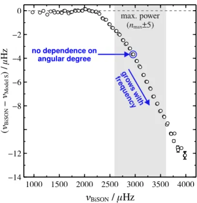
at the meteoritic age of the solar system. We take Model S [5] as an example. If we compute the linear adiabatic mode frequencies of this model and compare them with observed values [e.g. the low-degree data from the Birmingham So-lar Oscillation Network, BiSON;3,4] we might hope that the differences between observed and modelled frequencies
are randomly scattered about zero.
Instead, one gets the values plotted in Fig. 1. The white points indicate the differences between the mode
frequencies predicted for Model S and those observed by BiSON. The discrepancy is much larger than the quoted uncertainties but it is also not random, and its structure tells us something about where the problem arises. First, the frequency differences do not depend on the angular
degree , which suggests that the discrepancy lies well above the modes’ lower turning points. The low-degree data alone only tells us that the cause is not very deep in the Sun but the frequency differences of the higher-degree
modes are also-independent. Because they have shal-lower shal-lower turning points, this suggests that the problem is quite close to the Sun’s surface. Second, the frequency differences are close to zero at frequencies below about
2200µHz. Higher-frequency modes have shallower
up-per turning points, which again implies that the problem is somewhere near the Sun’s surface. At 2200µHz, the
modes’ upper turning points are around 1 Mm below the surface, which implies that the effect really is confined to
the near-surface layers.
The shaded region in Fig.1indicates the range of fre-quency covering about five radial orders either side of the frequency of maximum oscillation powerνmax. This is the
range in which modes oscillate with the greatest power and are thus most easily observed. It shows that the sur-face effect probably affects nearly all the observed modes
in distant Sun-like stars, unlike the Sun, in which we ob-serve low-frequency modes that appear unaffected by the
surface effect. The best targets from the nominalKepler
mission have lowest mode frequencies equivalent to about 2300µHz in the Sun, which is within the range of affected
modes. For this reason, the surface effect is unavoidable:
when fitting stellar models to individual mode frequencies, somethingmustbe done about the surface effect. In the
case of the Sun, even the large separations of the modelled and observed frequencies differ by about 1µHz. When
applied to the standard scaling relations [6], this bias in the large separation corresponds to biases in mass and radius of about 3 and 1.5 per cent, respectively.1
1The scaling relations are in essence empirical, which suppresses this effect. But if the surface effect varies significantly between different stars, it could be important.
2.2 The physical cause
It may come as a surprise that we have a fairly good idea about what causes the surface effect: improper modelling
of near-surface convection. Most stellar models use some form of mixing-length theory (MLT), in which the con-vection zone is presumed to contain buoyantly-unstable rising and falling parcels of material (see Fig. 2, left). These parcels rise or fall by one mixing length, typically parametrized in terms of the local pressure scale height,
HP = −dr/d lnP, after which they disperse, mixing the
heat and composition of their origin into their new sur-roundings.
In reality, the flows are much more complicated, as is now understood from detailed 3D RHD simulations that ac-curately reproduce many observable features of convection at the Sun’s surface [see7, for an excellent review of the Sun’s surface convection]. Let us start with one of the slow upflows. As it rises and the density decreases, so the flow expands horizontally and, to conserve mass, part of it must turn over and join whatever downflows exist (see Fig.2, right). The rising plume ultimately appears as a granule at the surface, where the flows are chiefly horizontal. They then radiate heat to the vacuum of space before plummeting downward in narrow, turbulent intragranular lanes. Along the way back down, these downflows will draw material turning over from the widening upflows.
This is a very different picture from the calm rise and
fall of MLT’s parcels and it leads to a number of effects
that affect the mode frequencies. Following the thorough
discussion by Rosenthal [8], we can broadly divide these into two types of effect.Modelphysics includes everything
that is wrong with the background model that we perturb. This includes, but is not limited to, MLT’s incorrect tem-perature gradient, the incorrect atmospheric structure and the absence of turbulent pressure.Modalphysics includes everything that is wrong with the calculation of the mode frequencies, which are affected by the perturbation to the
turbulent pressure [e.g.9], the modification of wave speeds when travelling with or against the flows [e.g.10] and vari-ous effects of non-adiabaticity [e.g.11]. All of these effects
are most pronounced near the surface where convection becomes inefficient and the temperature gradient deviates
furthest from the adiabatic value.
That so many physical effects contribute to the surface
effect makes it a difficult problem to tackle piece by piece.
In working on one component, one might think the problem is solved, only to find that another component returns you to square one. But it is not hopeless! We can learn how much each component might contribute and gradually add them up, bearing in mind that as our models improve, we might sometimes veer further from the observations before once again closing the gap.
3 Parametrizations
The surface effect in Fig.1appears to be a relatively simple
2 The problem
2.1 Phenomenology of the surface effects
Suppose that one calibrates a solar model in the traditional sense by varying the mixing length parameter, initial he-lium abundance and initial metallicity to evolve a stellar model that matches the Sun’s current radius, luminosity and surface metallicity, with the mass fixed at 1 Mand the age
at the meteoritic age of the solar system. We take Model S [5] as an example. If we compute the linear adiabatic mode frequencies of this model and compare them with observed values [e.g. the low-degree data from the Birmingham So-lar Oscillation Network, BiSON;3,4] we might hope that the differences between observed and modelled frequencies
are randomly scattered about zero.
Instead, one gets the values plotted in Fig.1. The white points indicate the differences between the mode
frequencies predicted for Model S and those observed by BiSON. The discrepancy is much larger than the quoted uncertainties but it is also not random, and its structure tells us something about where the problem arises. First, the frequency differences do not depend on the angular
degree , which suggests that the discrepancy lies well above the modes’ lower turning points. The low-degree data alone only tells us that the cause is not very deep in the Sun but the frequency differences of the higher-degree
modes are also-independent. Because they have shal-lower shal-lower turning points, this suggests that the problem is quite close to the Sun’s surface. Second, the frequency differences are close to zero at frequencies below about
2200µHz. Higher-frequency modes have shallower
up-per turning points, which again implies that the problem is somewhere near the Sun’s surface. At 2200µHz, the
modes’ upper turning points are around 1 Mm below the surface, which implies that the effect really is confined to
the near-surface layers.
The shaded region in Fig.1indicates the range of fre-quency covering about five radial orders either side of the frequency of maximum oscillation powerνmax. This is the range in which modes oscillate with the greatest power and are thus most easily observed. It shows that the sur-face effect probably affects nearly all the observed modes
in distant Sun-like stars, unlike the Sun, in which we ob-serve low-frequency modes that appear unaffected by the
surface effect. The best targets from the nominalKepler
mission have lowest mode frequencies equivalent to about 2300µHz in the Sun, which is within the range of affected
modes. For this reason, the surface effect is unavoidable:
when fitting stellar models to individual mode frequencies, somethingmustbe done about the surface effect. In the
case of the Sun, even the large separations of the modelled and observed frequencies differ by about 1µHz. When
applied to the standard scaling relations [6], this bias in the large separation corresponds to biases in mass and radius of about 3 and 1.5 per cent, respectively.1
1The scaling relations are in essence empirical, which suppresses this effect. But if the surface effect varies significantly between different stars, it could be important.
2.2 The physical cause
It may come as a surprise that we have a fairly good idea about what causes the surface effect: improper modelling
of near-surface convection. Most stellar models use some form of mixing-length theory (MLT), in which the con-vection zone is presumed to contain buoyantly-unstable rising and falling parcels of material (see Fig. 2, left). These parcels rise or fall by one mixing length, typically parametrized in terms of the local pressure scale height, HP = −dr/d lnP, after which they disperse, mixing the heat and composition of their origin into their new sur-roundings.
In reality, the flows are much more complicated, as is now understood from detailed 3D RHD simulations that ac-curately reproduce many observable features of convection at the Sun’s surface [see7, for an excellent review of the Sun’s surface convection]. Let us start with one of the slow upflows. As it rises and the density decreases, so the flow expands horizontally and, to conserve mass, part of it must turn over and join whatever downflows exist (see Fig.2, right). The rising plume ultimately appears as a granule at the surface, where the flows are chiefly horizontal. They then radiate heat to the vacuum of space before plummeting downward in narrow, turbulent intragranular lanes. Along the way back down, these downflows will draw material turning over from the widening upflows.
This is a very different picture from the calm rise and
fall of MLT’s parcels and it leads to a number of effects
that affect the mode frequencies. Following the thorough
discussion by Rosenthal [8], we can broadly divide these into two types of effect.Modelphysics includes everything
that is wrong with the background model that we perturb. This includes, but is not limited to, MLT’s incorrect tem-perature gradient, the incorrect atmospheric structure and the absence of turbulent pressure.Modalphysics includes everything that is wrong with the calculation of the mode frequencies, which are affected by the perturbation to the
turbulent pressure [e.g.9], the modification of wave speeds when travelling with or against the flows [e.g.10] and vari-ous effects of non-adiabaticity [e.g.11]. All of these effects
are most pronounced near the surface where convection becomes inefficient and the temperature gradient deviates
furthest from the adiabatic value.
That so many physical effects contribute to the surface
effect makes it a difficult problem to tackle piece by piece.
In working on one component, one might think the problem is solved, only to find that another component returns you to square one. But it is not hopeless! We can learn how much each component might contribute and gradually add them up, bearing in mind that as our models improve, we might sometimes veer further from the observations before once again closing the gap.
3 Parametrizations
The surface effect in Fig.1appears to be a relatively simple
function of mode frequency only. Thus, several groups have proposed parametric forms for this function whose
b
ac
k
gr
ou
nd
hot cold
mixing length theory
slow updraft granule
ra
pi
d
d
ow
nd
ra
ft
3D RHD simulations
Figure 2:A crude illustration of the difference between the mixing-length theory of convection (MLT, left) and the structure of near-surface convection suggested by 3D RHD simulations (right). In MLT, buoyantly-unstable parcels of material retain their composition and heat content while floating upwards (or sinking downwards) by onemixing length lMLTbefore dispersing their composition and heat into their new surroundings. In the 3D RHD simulations, slow, broad upflows expand as they rise through layers of decreasing density, ultimately reaching the surface and manifesting as granules. At the surface, material cools and sinks back down between the granules in rapid, cool downdrafts that we see as intragranular lanes.
max. power (nmax±5)
power law cubic combined
modified Lorentzian BiSON - Model S
(
ν
–
νM
o
d
el
S
)
/
μ
H
z
−14 −12 −10 −8 −6 −4 −2 0
ν
BiSON /μ
Hz
1000 1500 2000 2500 3000 3500 4000
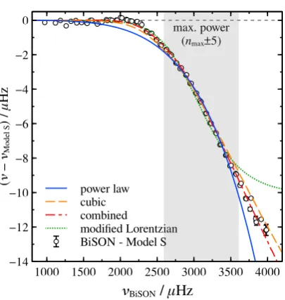
Figure 3: Frequency differences, as a function of frequency, for the observed surface effect in the Sun (white points) and several parametrizations (see Sec.3). The shaded region shows the frequency range over which the modes have their greatest power, as in Fig.1. The parametrizations shown are a power-law [solid blue, 12], the cubic and combined formulae [dashed orange and dash-dotted red, 13] and a modified Lorentzian [dotted green, 14].
parameters can be fit when comparing stellar models to ob-servations. Here I shall review the best known and compare them for the Sun.
First, Kjeldsen et al. [12] proposed that the surface ef-fect can be described as a power law with an index fixed to a solar-calibrated value (usually around 5 but slightly de-pendent on the precise physics of the stellar model). They also proposed that the magnitude of the power law be fit af-ter rescaling the frequencies so that the stellar model being compared has the same mean density as the observed star. To rescale the frequencies so, they propose using the ratio of the large separations. This simple parametrization has been widely used since its publication [e.g.15].
More recently, Ball & Gizon [13] proposed parametriza-tions based on surface perturbaparametriza-tions and the asymptotic behaviour of the eigenmodes. Roughly speaking, the dis-placement eigenfunctions are exponentially decaying func-tions near the photosphere and, combining them with the variational principle for the linear, adiabatic oscillation equations [16], one finds that, for a sound speed perturba-tion or pressure scale height perturbaperturba-tion near the surface, the frequency shifts go either likeν3/Iorν−1/I, whereν
is the mode frequency andIthe normalized mode inertia. These parametric forms, which Ball & Gizon [13] refer to as thecubicandinverseterms, respectively, were originally derived by Gough [17]2 in a discussion of the Sun’s
fre-quency shifts over the magnetic activity cycle. The inverse term alone does not fit the data well so Ball & Gizon [13] proposed to combine it with the cubic term, giving what they call thecombinedsurface correction.
Most recently, Sonoi et al. [14] proposed to describe the surface effect as a modified Lorentzian function and
calibrated its parameters to frequency shifts induced by replacing the near-surface layers of stellar models with averaged data from hydrodynamics simulations (see Sec.4,
below). This parametrization is very new and has not yet been tested on observed data.
Fig.3shows the same data as Fig.1(BiSON against Model S), along with the above-mentioned parametriza-tions. The power law fit performs reasonably well in the shaded range around νmax but overestimates the surface
effect both where it begins to rise and at higher frequencies.
The cubic and the combined terms fare better. Though the improvement by using the combined term (rather than just the cubic term) is significant for the Sun, this was not the case for the COROT target HD 52265 studied by Ball & Gizon [13]. Finally, the modified Lorentzian captures most of the low-frequency behaviour but underestimates the difference at high frequencies.
Though different in principle, it is worth mentioning
several methods proposed by Roxburgh (and Vorontsov in earlier work) [20–22]. These are all based on represent-ing the oscillation modes as simple oscillations with phase shifts at the inner and outer boundaries. The outer phase shift contains the undesired and presumably-independent surface term whereas the inner phase shift is related to the structure of the stellar core. One can combine the fre-quencies into ratios of differences or so-calledseparation
ratiosthat are nearly independent of the near-surface layers
[20]. Otí Floranes et al. [23] computed kernels for these quantities and demonstrated that they are, indeed, largely insensitive to the near-surface layers and they have seen widespread use in asteroseismic modelling. From the same underlying principles, Roxburgh [21,22] described meth-ods to fit out a more general-independent component of the frequency differences. These are too new to have been
used widely.
These various parametrized methods have not yet been systematically compared with observations, though the community’s collective experience suggests that none gen-erally leads to absurd results. Schmitt & Basu [24] con-ducted the most thorough study yet by inserting structural perturbations into stellar models across the HR diagram and then trying to fit the frequency differences using the
solar-calibrated power law, the cubic and combined terms of Ball & Gizon [13] or the observed solar surface effect,
rescaled by the large separation. The combined term by Ball & Gizon [13] appeared to fare best, although the scaled solar term also performed reasonably on the main sequence.
The parametrizations do not solve the problem of the surface effects but they at least allow us to exploit the reams
of data already available while we work towards properly modelling the surface effects. The results should always
be interpreted with the knowledge that the Sun remains the only star for which we can truly calibrate the frequency differences. Everything else depends on the confidence we
place in how well our best-fitting models represent the stars under study.
4 Three-dimensional radiation
hydrodynamics
I mentioned in Sec.2that the surface effect is chiefly caused
by improper modelling of near-surface convection. So why
BiSON – Model S BiSON – MURaM(z) MURaM(z) – Model S MURaM(P) – Model S MURaM(τ) – Model S
(
ν1
–
ν2
)
/
μ
H
z
2
0
−2
−4
−6
−8
−10
−12
ν / μHz
1000 1500 2000 2500 3000 3500 4000
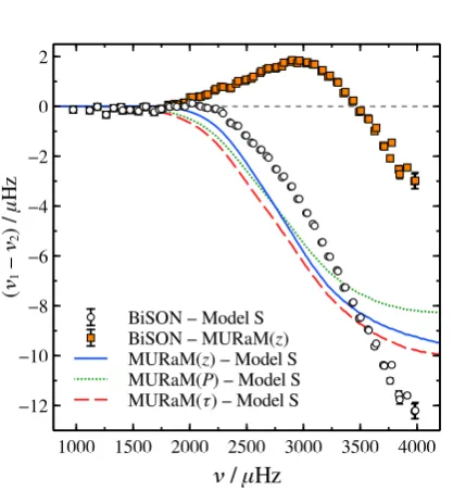
Figure 4: Frequency differences for the Sun between different
combinations of models and data as a function of model frequen-cies. The lines show the frequency differences between the solar
model before and after the near-surface layers are replaced by horizontally-averaged 3D RHD simulation data. The different
lines correspond to different choices of averaging co-ordinate:
ge-ometric depthz(solid blue), pressureP(dotted green) or optical depthτ(dashed red). The white points show the same differences
between observed and modelled frequencies as in Fig.1. The or-ange squares show the frequency differences after the near-surface
layers of the solar model have been replaced by 3D RHD simu-lation data averaged at constant geometric depthz. The overall extent of the surface effect is reduced to a fewµHz but a clear
systematic difference remains.
not use better models of near-surface convection? This is the idea behind recent efforts to combine stellar models
with 3D RHD simulations. Several groups have simulated near-surface convection from first principles in stars of various spectral types [e.g.27–29]. These simulations are sufficiently realistic to reproduce most of the observed
char-acteristics of the Sun’s near-surface convection [again, see
7, for a review] and it is assumed that they are similarly realistic for other stars.
The process of replacing a stellar model’s near-surface layers with averaged simulation data is becoming known
aspatching. The frequency differences are then computed
between thepatchedmodel (the original stellar model) and
thepatchedmodel (with the near-surface layers replaced).
The idea of patching is not new. Rosenthal et al. [9] restricted their study of solar oscillations to modes with angular degree >60. These modes are trapped within the
solar convection zone, so they could compare their aver-aged simulation data with envelope models computed using MLT. Their early results showed that replacing the equilib-rium structure of the stellar model with the simulation data, averaged at constant geometric depth, already introduced a surface effect of similar magnitude to the observed effect,
below). This parametrization is very new and has not yet been tested on observed data.
Fig.3shows the same data as Fig.1(BiSON against Model S), along with the above-mentioned parametriza-tions. The power law fit performs reasonably well in the shaded range around νmax but overestimates the surface
effect both where it begins to rise and at higher frequencies.
The cubic and the combined terms fare better. Though the improvement by using the combined term (rather than just the cubic term) is significant for the Sun, this was not the case for the COROT target HD 52265 studied by Ball & Gizon [13]. Finally, the modified Lorentzian captures most of the low-frequency behaviour but underestimates the difference at high frequencies.
Though different in principle, it is worth mentioning
several methods proposed by Roxburgh (and Vorontsov in earlier work) [20–22]. These are all based on represent-ing the oscillation modes as simple oscillations with phase shifts at the inner and outer boundaries. The outer phase shift contains the undesired and presumably-independent surface term whereas the inner phase shift is related to the structure of the stellar core. One can combine the fre-quencies into ratios of differences or so-calledseparation
ratiosthat are nearly independent of the near-surface layers
[20]. Otí Floranes et al. [23] computed kernels for these quantities and demonstrated that they are, indeed, largely insensitive to the near-surface layers and they have seen widespread use in asteroseismic modelling. From the same underlying principles, Roxburgh [21,22] described meth-ods to fit out a more general-independent component of the frequency differences. These are too new to have been
used widely.
These various parametrized methods have not yet been systematically compared with observations, though the community’s collective experience suggests that none gen-erally leads to absurd results. Schmitt & Basu [24] con-ducted the most thorough study yet by inserting structural perturbations into stellar models across the HR diagram and then trying to fit the frequency differences using the
solar-calibrated power law, the cubic and combined terms of Ball & Gizon [13] or the observed solar surface effect,
rescaled by the large separation. The combined term by Ball & Gizon [13] appeared to fare best, although the scaled solar term also performed reasonably on the main sequence.
The parametrizations do not solve the problem of the surface effects but they at least allow us to exploit the reams
of data already available while we work towards properly modelling the surface effects. The results should always
be interpreted with the knowledge that the Sun remains the only star for which we can truly calibrate the frequency differences. Everything else depends on the confidence we
place in how well our best-fitting models represent the stars under study.
4 Three-dimensional radiation
hydrodynamics
I mentioned in Sec.2that the surface effect is chiefly caused
by improper modelling of near-surface convection. So why
BiSON – Model S BiSON – MURaM(z) MURaM(z) – Model S MURaM(P) – Model S MURaM(τ) – Model S
( ν1 – ν2 ) / μ H z 2 0 −2 −4 −6 −8 −10 −12
ν / μHz
1000 1500 2000 2500 3000 3500 4000
Figure 4: Frequency differences for the Sun between different
combinations of models and data as a function of model frequen-cies. The lines show the frequency differences between the solar
model before and after the near-surface layers are replaced by horizontally-averaged 3D RHD simulation data. The different
lines correspond to different choices of averaging co-ordinate:
ge-ometric depthz(solid blue), pressureP(dotted green) or optical depthτ(dashed red). The white points show the same differences
between observed and modelled frequencies as in Fig.1. The or-ange squares show the frequency differences after the near-surface
layers of the solar model have been replaced by 3D RHD simu-lation data averaged at constant geometric depthz. The overall extent of the surface effect is reduced to a fewµHz but a clear
systematic difference remains.
not use better models of near-surface convection? This is the idea behind recent efforts to combine stellar models
with 3D RHD simulations. Several groups have simulated near-surface convection from first principles in stars of various spectral types [e.g.27–29]. These simulations are sufficiently realistic to reproduce most of the observed
char-acteristics of the Sun’s near-surface convection [again, see
7, for a review] and it is assumed that they are similarly realistic for other stars.
The process of replacing a stellar model’s near-surface layers with averaged simulation data is becoming known
aspatching. The frequency differences are then computed
between thepatchedmodel (the original stellar model) and
thepatchedmodel (with the near-surface layers replaced).
The idea of patching is not new. Rosenthal et al. [9] restricted their study of solar oscillations to modes with angular degree >60. These modes are trapped within the
solar convection zone, so they could compare their aver-aged simulation data with envelope models computed using MLT. Their early results showed that replacing the equilib-rium structure of the stellar model with the simulation data, averaged at constant geometric depth, already introduced a surface effect of similar magnitude to the observed effect,
although a significant systematic effect remained. More
Ball et al. Sonoi et al. BaSTI (0.6–2.0 M⊙)
lo
g
g
2.5 3.0 3.5 4.0 4.5 5.0Teff
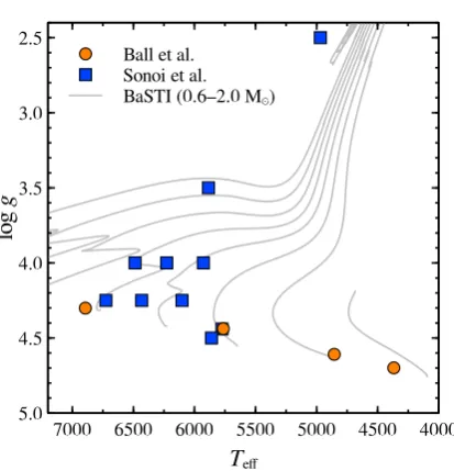
4000 4500 5000 5500 6000 6500 7000Figure 5:Kiel diagram (surface gravity against effective
tempera-ture) showing the parameters of the 3D RHD simulations used by [14, blue squares] and [25, orange circles]. The grey lines show solar-metallicity evolutionary tracks from BaSTI [26] for masses from 0.6 to 2.0 Min steps of 0.2 M. Both sets of simulations
include a solar model (models A and G2 in Sonoi et al. [14] and Ball et al. [25]) and the hottest models (models B and F3 in Sonoi et al. [14] and Ball et al. [25]) also have comparable parameters.
recently, Piau et al. [30] used 3D RHD simulation data to compute surface effects in a complete solar model (not just
the convective envelope), finding that the structural compo-nent of the surface effect reduced the remain discrepancy to
a few µHz. Finally, on the subject of the solar surface
cor-rection, Magic & Weiss [31] computed surface effects using
simulations with different input magnetic field strengths
and found that they could reproduce reasonably well the frequency shifts induced by the changing level of magnetic activity in the Sun.
The 12 months preceding this meeting saw the first papers to combine stellar models and 3D RHD simulations for the surface effects in other types of star. First, Sonoi
et al. [14] combined stellar models from CESTAM [32,
33] with simulations from the CIFIST atmosphere grid [27]. Second, Ball et al. [25] combined stellar models from MESA [34–36] with simulations from the MURaM code [28]. The two groups independently performed nearly the same calculations using somewhat complementary sets of stellar models. The ten simulations used by Sonoi et al. [14] cover one red giant (around the red clump) and dwarfs and subgiants hotter than the Sun. The four simulations used by Ball et al. [25] span the main-sequence from spectral type F3 to K5. Fig.5shows the atmospheric parameters for the two groups’ simulations.
These studies are not definitive. For a start, they only deal with the part of the surface effect caused by improving
the structure of the equilibrium stellar model. The aver-aged simulation profiles include the turbulent pressure but
it remains unclear what is the appropriate form of the per-turbation to the turbulent pressure. Both Sonoi et al. [14] and Ball et al. [25] assume that the turbulent pressure varies with the total pressure: Rosenthal et al. [9] dubbed this the
gas gamma oneapproximation. Changing this assumption
potentially affects the results by a factor of about two [9].
Moreover, it is unclear exactly what is the appropriate hori-zontal average to take from the simulation data. Sonoi et al. [14] and Ball et al. [25] both used averages over constant geometric depth but different averages give surface effects
that differ by a few µHz for the Sun (see Fig.4).
Fig.4shows how the mode frequencies of a standard solar model [Model S again,5] are changed by the mod-ification of the near-surface equilibrium structure. The white points are the same differences shown in Figs1and
3. The solid blue, dotted green and dashed red curves are the differences in the model frequencies before and after
patching with the G2-type MURaM simulation averaged over constant geometric depth, pressure or optical depth. The spread in the curves shows that uncertainty above the appropriate average introduces an uncertainty in the fre-quency shifts of about 0.5–1.0µHz. Finally, the orange squares show the remaining difference between the patched
model (with the simulation averaged at constant geometric depth) and the BiSON observations. The overall surface effect is reduced substantially, though clearly a large effect
remains and the remaining difference is still a surface effect.
It is not yet clear if the remaining trend is because the aver-aged near-surface structure is still not quite right, because non-adiabatic effects have been neglected, or (most likely)
both.
With these uncertainties in mind, both teams found that the surface effect is larger in stars that are hotter. Based
on their cooler dwarfs, Ball et al. [25] also noted that the overall shape of the frequency differences as a function of
frequency is similar in the G2-, K0- and K5-type models, but some qualitative change sets in between the F3- and G2-type models. Sonoi et al. [14], with their greater coverage of surface gravity, also found that the surface effect increases
with increasing surface gravity. Within their limitations, the two groups’ results are mutually consistent. They have two simulations with similar parameters and the results agree well. Fig. 6shows the frequency shifts for all the simulations by Ball et al. [25, left] and the simulations A and B of Sonoi et al. [14, right], which have similar parameters to models G2 and F3 of Ball et al. [25].
Both teams also compared the parametric fits described in Sec. 3, though Sonoi et al. [14] only compared their modified Lorentzian with a power law. Fig.6shows that a simple power law does not describe the differences
K5 K0
G2
F3 K5
K0 G2 F3
(
ν3D
R
H
D
–
ν1D
)/
μ
H
z
−30 −25 −20 −15 −10 −5 0
ν
/
ν
ac0 0.2 0.4 0.6 0.8 1
A
B A
B
ν
/
ν
ac0 0.2 0.4 0.6 0.8 1
Figure 6: Frequency differences between various models before and after their near-surface layers are replaced with
horizontally-averaged 3D RHD simulation profiles, as a function of frequency normalized to the acoustic cut-offfrequency. The left panel shows
models from Ball et al. [25]; the right panel for models from Sonoi et al. [14, adapted from their Fig. 3]. The models labelled A and B on the right correspond to the solar model and hottest model of Sonoi et al. [14] and can be compared to models G2 and F3 on the left, respectively.
Further exploitation of the 3D RHD simulations is un-derway, notably on non-adiabatic effects, but these early
results already give some indication of how much of a surface effect is introduced by improving the background
stellar model. It remains to be seen if the conclusions hold up as further surface effects are considered.
5 The future
To close, I briefly opine on how we might progress further on the problem of surface effects. The main theoretical
path at this point is to further exploit the 3D RHD simula-tions. There is far more information available than simply the horizontally- and temporally-averaged profiles and this information can be used to investigate other components of the surface effect. But it should be remembered that
even indirect conclusions drawn from the simulations can be useful. For example, the parametrizations of the surface effects tend to correlate with the mixing-length parameter
in stellar models. There is good physical reason for this: both the surface effect and the mixing-length parameter are
sensitive to the superadiabatic layer near the stellar surface. If the mixing-length parameter is constrained separately by the simulations [e.g.37,38] then the surface effect is also
better constrained.
Progress is more difficult from the observational side.
The best solar-like oscillators from the nominal Kepler
mission show modes oscillating at frequencies nearly low enough that they are unaffected by the surface effect. If
just a few more radial orders could be detected, these low frequencies could potentially be used to fit models
with-out a surface term, though at the cost of discarding the many higher-frequency modes that are available. Alas, no imminent mission will provide such high-quality data for single targets, so we may have to wait until PLATO [39] for higher-quality data on single targets.
From the ground, however, there is tremendous poten-tial from the Stellar Oscillation Network Group [see e.g.
40, these proceedings]. Because it observes in radial veloc-ity, the background signal of granulation is weaker, which allows lower-frequency modes to be detected more eas-ily. This could allow us to calibrate models directly to the unaffected frequencies and inspect the remaining
frequen-cies to determine the surface effect after fitting the stellar
model. One node of the network is fully operational and another partially so. The first results from the first node were reported at this meeting [40]. Adding nodes to the network probably represents our best chance of bringing tight observational constraints to bear on the problem of surface effects.
Acknowledgement
The author would like to thank the organizers for partial finan-cial support to attend the meeting. He also acknowledges re-search funding by Deutsche Forschungsgemeinschaft (DFG) un-der grant SFB 963/1 “Astrophysical flow instabilities and
turbu-lence”, Projects A18.
References
[1] M. Auvergne, P. Bodin, L. Boisnard, J.T. Buey, S. Chaintreuil, G. Epstein, M. Jouret, T. Lam-Trong,
P. Levacher, A. Magnan et al., A&A,506, 411 (2009),
0901.2206
[2] W.J. Borucki, D. Koch, G. Basri, N. Batalha, T. Brown, D. Caldwell, J. Caldwell, J. Christensen-Dalsgaard, W.D. Cochran, E. DeVore et al., Science
327, 977 (2010)
[3] A.M. Broomhall, W.J. Chaplin, G.R. Davies, Y. Elsworth, S.T. Fletcher, S.J. Hale, B. Miller, R. New, MNRAS,396, L100 (2009),0903.5219
[4] G.R. Davies, W.J. Chaplin, Y. Elsworth, S.J. Hale, MNRAS,441, 3009 (2014),1405.0160
[5] J. Christensen-Dalsgaard, W. Dappen, S.V. Ajukov, E.R. Anderson, H.M. Antia, S. Basu, V.A. Baturin, G. Berthomieu, B. Chaboyer, S.M. Chitre et al., Sci-ence272, 1286 (1996)
[6] H. Kjeldsen, T.R. Bedding, A&A293, 87 (1995),
arXiv:astro-ph/9403015
[7] Å. Nordlund, R.F. Stein, M. Asplund, Living Reviews in Solar Physics6(2009)
[8] C.S. Rosenthal,Convective Effects on Mode
Frequen-cies, inSCORe’96 : Solar Convection and
Oscilla-tions and their RelaOscilla-tionship, edited by F.P. Pijpers,
J. Christensen-Dalsgaard, C.S. Rosenthal (1997), Vol. 225 ofAstrophysics and Space Science Library, pp. 145–160
[9] C.S. Rosenthal, J. Christensen-Dalsgaard, Å. Nord-lund, R.F. Stein, R. Trampedach, A&A, 351, 689 (1999),astro-ph/9803206
[10] T.M. Brown, Science226, 687 (1984)
[11] G. Houdek, Ph.D. Thesis, Formal- und Naturwiss-eschaftliche Fakultät der Universität Wien, (1996) (1996)
[12] H. Kjeldsen, T.R. Bedding, J. Christensen-Dalsgaard, ApJL,683, L175 (2008),0807.1769
[13] W.H. Ball, L. Gizon, A&A, 568, A123 (2014),
1408.0986
[14] T. Sonoi, R. Samadi, K. Belkacem, H.G. Ludwig, E. Caffau, B. Mosser, A&A, 583, A112 (2015), 1510.00300
[15] V. Silva Aguirre, S. Basu, I.M. Brandão, J. Christensen-Dalsgaard, S. Deheuvels, G. Do˘gan, T.S. Metcalfe, A.M. Serenelli, J. Ballot, W.J. Chaplin et al., ApJ,769, 141 (2013),1304.2772
[16] P. Ledoux, T. Walraven, Handbuch der Physik51, 353 (1958)
[17] D.O. Gough,Comments on Helioseismic Inference, in
Progress of Seismology of the Sun and Stars, edited by
Y. Osaki, H. Shibahashi (1990), Vol. 367 ofLecture
Notes in Physics, Berlin Springer Verlag, p. 283
[18] K.G. Libbrecht, M.F. Woodard, Nature, 345, 779 (1990)
[19] P. Goldreich, N. Murray, G. Willette, P. Kumar, ApJ,
370, 752 (1991)
[20] I.W. Roxburgh, S.V. Vorontsov, A&A, 411, 215 (2003)
[21] I.W. Roxburgh, A&A,574, A45 (2015),1406.6491
[22] I.W. Roxburgh, A&A,585, A63 (2016)
[23] H. Otí Floranes, J. Christensen-Dalsgaard, M.J. Thompson, MNRAS,356, 671 (2005)
[24] J.R. Schmitt, S. Basu, ApJ, 808, 123 (2015),
1506.06678
[25] W.H. Ball, B. Beeck, R.H. Cameron, L. Gizon, A&A,
592, A159 (2016),1606.02713
[26] A. Pietrinferni, S. Cassisi, M. Salaris, F. Castelli, ApJ,
612, 168 (2004),astro-ph/0405193
[27] H.G. Ludwig, E. Caffau, M. Steffen, B. Freytag,
P. Bonifacio, A. Kuˇcinskas, Mem. Soc. Astron. Ital-iana,80, 711 (2009),0908.4496
[28] B. Beeck, R.H. Cameron, A. Reiners, M. Schüssler, A&A,558, A48 (2013),1308.4874
[29] Z. Magic, R. Collet, M. Asplund, R. Trampedach, W. Hayek, A. Chiavassa, R.F. Stein, Å. Nordlund, A&A,557, A26 (2013),1302.2621
[30] L. Piau, R. Collet, R.F. Stein, R. Trampedach, P. Morel, S. Turck-Chièze, MNRAS,437, 164 (2014),
1309.7179
[31] Z. Magic, A. Weiss, A&A, 592, A24 (2016),
1606.01030
[32] P. Morel, A&AS,124(1997)
[33] P. Morel, Y. Lebreton, Ap&SS, 316, 61 (2008),
0801.2019
[34] B. Paxton, L. Bildsten, A. Dotter, F. Herwig, P. Lesaf-fre, F. Timmes, ApJS,192, 3 (2011),1009.1622
[35] B. Paxton, M. Cantiello, P. Arras, L. Bildsten, E.F. Brown, A. Dotter, C. Mankovich, M.H. Montgomery, D. Stello, F.X. Timmes et al., ApJS,208, 4 (2013),
1301.0319
[36] B. Paxton, P. Marchant, J. Schwab, E.B. Bauer, L. Bildsten, M. Cantiello, L. Dessart, R. Farmer, H. Hu, N. Langer et al., ApJS, 220, 15 (2015),
1506.03146
[37] H.G. Ludwig, B. Freytag, M. Steffen, A&A,346, 111
(1999),astro-ph/9811179
[38] R. Trampedach, R.F. Stein, J. Christensen-Dalsgaard, Å. Nordlund, M. Asplund, MNRAS, 445, 4366 (2014),1410.1559
[39] H. Rauer, C. Catala, C. Aerts, T. Appourchaux, W. Benz, A. Brandeker, J. Christensen-Dalsgaard, M. Deleuil, L. Gizon, M.J. Goupil et al., Experimental Astronomy38, 249 (2014),1310.0696
[40] J. Christensen-Dalsgaard,200 nights withµHerculis:
early results from the SONG Hertzsprung telescope,
inSeismology of the Sun and the Distant Stars 2016,