Original citation:
Zhao, B. (2012). Hard-input-hard-output capacity analysis of UWB BPSK systems with timing errors. IEEE Transactions on Vehicular Technology, 61(4), pp. 1741-1751.
Permanent WRAP url:
http://wrap.warwick.ac.uk/49533
Copyright and reuse:
The Warwick Research Archive Portal (WRAP) makes the work of researchers of the University of Warwick available open access under the following conditions. Copyright © and all moral rights to the version of the paper presented here belong to the individual author(s) and/or other copyright owners. To the extent reasonable and practicable the material made available in WRAP has been checked for eligibility before being made available.
Copies of full items can be used for personal research or study, educational, or not-for-profit purposes without prior permission or charge. Provided that the authors, title and full bibliographic details are credited, a hyperlink and/or URL is given for the original metadata page and the content is not changed in any way.
Publisher’s statement:
“© 2012 IEEE. Personal use of this material is permitted. Permission from IEEE must be obtained for all other uses, in any current or future media, including
reprinting/republishing this material for advertising or promotional purposes, creating new collective works, for resale or redistribution to servers or lists, or reuse of any copyrighted component of this work in other works.”
Zhao, B. (2012). Hard-input-hard-output capacity analysis of UWB BPSK systems with timing errors. IEEE Transactions on Vehicular Technology, 61(4), pp. 1741-1751. http://dx.doi.org/10.1109/TVT.2012.2188418
A note on versions:
The version presented here may differ from the published version or, version of record, if you wish to cite this item you are advised to consult the publisher’s version. Please see the ‘permanent WRAP url’ above for details on accessing the published version and note that access may require a subscription.
Hard-Input-Hard-Output Capacity Analysis of
UWB BPSK Systems With Timing Errors
Bo Zhao, Yunfei Chen, Senior Member, IEEE, Roger J. Green, Senior Member, IEEE
Corresponding Address:
Yunfei Chen
School of Engineering
University of Warwick, Coventry, U.K. CV4 7AL
Tel: +44 (0)24 765 23105, e-mail:
[email protected]
Abstract
The hard-input-hard-output capacity of a binary phase shift keying ultra-wide bandwidth system
is analyzed for both additive white Gaussian noise and multipath fading channels with timing errors.
Unlike previous works that calculate the capacity with perfect synchronization and/or with multiple
access interference only, our analysis consider timing errors with different distributions as well as
the inter-path, inter-chip and inter-symbol interferences, as in practical systems. The sensitivity of the
channel capacity to the timing error is examined. The effects of pulse shape, multiple access technique,
number of users and number of chips are studied. It is found that time-hopping is less sensitive to the
pulse shape and the timing error with higher capacity than direct-sequence due to its low duty of cycle.
Using these results, one can choose appropriate system parameters for different applications.
Index Terms
Channel capacity, synchronization, timing error, ultra-wide bandwidth.
I. INTRODUCTION
In recent years, ultra-wide bandwidth (UWB) technology has attracted great research interest
from both academia and industry [1] [2]. Due to its very low transmission power, UWB is able
to minimize interferences to coexist with other wireless systems in the same band. Thus, it is a
very promising solution to wireless personal area networks and wireless sensor networks. In [3]
- [6], performances of UWB systems have been analyzed in terms of the bit error rate (BER)
and the signal-to-interference-plus-noise-ratio (SINR). In addition to BER and SINR, channel
capacity is also an important performance measure that determines the maximum achievable
information rate in a UWB system. Many researchers have analyzed the channel capacity for
different UWB systems to provide useful engineering insights.
Based on the results for optical channels in [7], the channel capacity of an M-ary pulse
position modulation (PPM) UWB system was evaluated in [8] for additive white Gaussian noise
(AWGN) channels with a single user. For the same system, authors in [9] showed that the channel
capacity is highly affected by pulse shapes. By modeling the multiple access interference (MAI)
as Gaussian, the analysis on the channel capacity was extended to AWGN channels with multiple
users in [10] - [13]. In [14], the channel capacities of pulse amplitude modulation (PAM) and
PPM were compared over AWGN channels, where the MAI was also modeled as Gaussian. A
different approximation that approximates the characteristic function of the MAI was adopted to
evaluate the channel capacity of a binary PPM system in [15] and [16]. In addition, expressions
for the channel capacities of direct sequence code division multiple access (DS-CDMA) and
time-hopping (TH) PPM UWB systems were derived and compared in [17]. All these works calculate
the channel capacity for AWGN channels. For multipath fading channels, the channel capacity
has been analyzed for different UWB systems in [18] - [21]. It was shown in [18] and [19] that
the random path energy and correlation in multipath fading channels cause significant capacity
loss compared with the channel capacity in AWGN channels. Also, the inter-frame interference
However, none of the aforementioned works has taken all the necessary interferences into
account. It was reported in [22] that, in addition to the MAI, the inter-symbol interference (ISI),
the inter-path interference (IPI) and the inter-chip interference (ICI) (or inter-frame interference)
have significant effects on the performances of UWB systems too. The ISI is caused by
dis-placements of different symbols, the ICI is caused by disdis-placements of different chips in one
symbol, while the IPI is caused by displacements of different multipath components in one chip.
Also, stringent timing requirement is always a crucial issue for UWB communications, owing to
the narrow pulse and the low transmission power. However, none of the aforementioned works
has taken the timing error into account. It was shown in [23] that timing errors cause significant
performance degradation to the BER. The same degradation to the symbol error rate was observed
in [24] when time jitter is present. The degradation to channel capacity was not considered in
[24] but will be presented in our work. In [25], the authors showed that this degradation can
be reduced by choosing optimal processing gains for TH UWB systems. Similar degradations
may also be observed for capacity. In [26], the impact of desynchronization between the local
template and the received signal on the channel capacity was analyzed for UWB PPM systems
over an AWGN channel with a single user. There still lacks a complete analysis of the channel
capacity for UWB systems in the presence of timing errors corrupted by different interferences.
In this paper, we evaluate the capacity of DS and TH binary phase shift keying (BPSK)
UWB systems in the presence of timing errors for a multi-user environment. Similar to
[8]-[20], hard-input and hard-output capacity is calculated in our work. For simplicity, we refer
to it as capacity in the following. Both AWGN and multipath fading channels are studied. In
addition to the MAI, as in [14] - [16], the IPI, ICI and ISI are also considered. As well, different
distributions of the timing error are examined for different pulse shapes. Numerical results show
that the timing error can cause significant performance degradation in terms of channel capacity
and that the amount of the degradation depends on several factors, including the distribution of
the timing error, the pulse shape, the number of users and the number of chips. Although the
providing engineers with insights and guidelines on the system design, for example, the number
of users adopted in certain conditions.
II. DS UWB
In this section, we will evaluate the capacity of a multi-user DS BPSK UWB system over
AWGN and multipath fading channels. The transmitted signal of thek-th user can be expressed
as
s(trk)(t) =
∞
X
m=−∞
Nc−1 X
n=0
b(mk)β( k)
n g(t−mTb−nTc) (1)
where b(mk) is the m-th data symbol of the k-th user and bm(k) = −1 or b(mk) = +1 with equal
probabilities, βn(k) is the spreading code of the n-th frame of the k-th user and βn(k) = −1 or
βn(k) = +1 with equal probabilities, Tc is the chip interval, Nc is the number of chips in each
symbol, Tb =NcTc is the symbol interval, and g(t) is the monocycle pulse with energy Eg and
duration Dg. Denote Rg(·) as the normalized autocorrelation function of g(t), normalized with
respect to Eg, and Rg(Θ)≈0 whenΘ≥Dg orΘ≤ −Dg. In order to show that the sensitivity
of channel capacity to the timing error is affected by the pulse shape, rectangular pulse, the
second-order derivative Gaussian pulse and the fourth-order derivative Gaussian pulse are used
as examples in our analysis. Then, one has
Rg(Θ) =
1− |DΘ|
g, 0≤ |Θ| ≤Dg
0, otherwise
when the rectangular pulse is used,
Rg(Θ) =
"
1−4π
Θ
ν
2
+ 4π 2 3 Θ ν 4#
e−π(Θν)
2
when the second-order derivative Gaussian pulse is used, and
Rg(Θ) =
"
1−8π
Θ
ν
2
+ 8π2
Θ
ν
4
− 896π 3 420 Θ ν 6
+ 64π 4 420 Θ ν 8#
e−π(Θν)
2
when the fourth-order derivative Gaussian pulse is used, where ν is a time scale factor. Assume
A. AWGN channel
Consider an AWGN channel first. Without loss of generality, the first user is treated as the
desired user. Its superscript will be dropped for convenience in the following. Then, the received
signal of the desired user is given by
r(t) =A
∞
X
m=−∞
Nc−1 X
n=0
bmβng(t−mTb−nTc−τ) + Nu X
k=2
r(k)(t) +n(t) (2)
where r(k)(t) =A(k)s(k)
tr (t−τ(k))is the interfering signal from the k-th user, n(t) is the AWGN
with mean zero and standard deviation σ, τ and τ(k) are the transmission delays of the desired
user and the k-th user, respectively, A and A(k) are channel gains of the desired user and the
k-th user, respectively. It is assumed that the interfering users have the same signal energy as
the desired user through power control [27] and that τ(k) is uniformly distributed over [0, T b).
When symbol-by-symbol detection is conducted, the memory in the channel does not need to
be considered in the detection.
The receiver template for the detection of the m-th symbol of the desired user is given by˜
v(t) = Nc−1
X
n′=0
βn′g(t−n′Tc−mT˜ b−τˆ), (3)
where τˆ is the timing estimate for the desired user. The output of the correlator can be derived
as
R =
Z ( ˜m+1)Tb+ˆτ
˜ mTb+ˆτ
r(t)v(t)dt=bm˜S+I+ Nu X
k=2
M AI(k)
u +N (4)
whereS is the desired signal component,I =ISI+ICI includes the ICI and the ISI caused by
the timing errorǫ=τ−τ,ˆ M AIu(k) is the MAI from the k-th user and N is the noise component
with
S =ANcEgRg(ǫ), (5)
ISI =Egbm˜−1AβNc−1β0Rg(Tc−ǫ), ICI =Egbm˜ARg(Tc −ǫ)
Nc−2 X
n=0
βnβn+1, (6)
M AIu(k)=Eg
∞
X
m=−∞
Nc−1 X
n=0 Nc−1
X
n′=0
b(mk)A( k)β(k)
It can also be shown that the variance ofN isZ =V ar{N}=σ2N
cEg. Note that previous works
on capacity analysis ignored I. Note also that the desired signal component will disappear when
ǫ≥ Dg or ǫ ≤ −Dg, as Rg(ǫ)≈0 in this case. The conditional means, E{S2|ǫ} and E{I2|ǫ},
and the value ofE{M AIu(k) 2
}are calculated in Appendix A. For simplicity, the interference plus
noise term is modeled as Gaussian. It will be shown later that, for both DS and TH systems, this
approximation provides enough accuracy for our capacity analysis, and that it does not affect the
analysis of the effect of the timing error on the channel capacity. Then, the conditional average
BER, conditioned on ǫ, is derived as
Pe(ǫ) =Q
s
E{S2|ǫ}
E{I2|ǫ}+E{Z}+ (N
u−1)E{M AI( k) u
2 }
!
. (8)
The capacity of a discrete memoryless channel using BPSK is given by [31]
C = max P(xj)
1
X
j=0 1
X
i=0
P(xj)P(yi|xj) log
P(yi|xj)
P(yi)
, (9)
wherexj represents the input symbols andyi represents the output symbols. The maximum value
of (9) is achieved when the system has equally likely input symbols in the binary modulation
scheme [10], [19]. Therefore, the channel capacity for the desired user can be calculated as
C(ǫ) = 1 + (1−Pe(ǫ)) log2(1−Pe(ǫ)) +Pe(ǫ) log2Pe(ǫ). (10)
Note from (9) that the channel capacity is determined by the transition probability, which depends
on the BER. Since the BER is a function of the timing error in the analysis, the channel capacity
is also parametrized by ǫ when the timing error exists. By averaging (10) over ǫ, the channel
capacity of the desired user can be calculated as
¯
CAW GN =
Z ∞
−∞
C(x)pǫ(x)dx (11)
where pǫ(x) is the probability density function (PDF) of the timing error. Similar to [12], it is
assumed that each user contributes a fraction of the traffic in the channel, so the total capacity is
estimated by aggregating the channel capacity of each user. Then, in a multi-user environment,
the total channel capacity can be estimated as [12]
ˆ
One sees that CˆAW GN is proportional to the number of users Nu. But since C¯AW GN decreases
withNu, as can be seen from (8) to (11), the total capacity will be conpromised by MAI. Using
(8) and (10), the channel capacity of the desired user for the DS-BPSK UWB system in an
AWGN channel can be calculated by (11), and the total channel capacity for the DS-BPSK
UWB system can be calculated by (12).
B. Multipath fading channel
Next, we will evaluate the capacity of the DS UWB system in a multipath fading channel with
multiple users. The channel impulse response of the k-th user is h(k)(t) = PL
l=0α (k)
l δ(t−τ (k) l )
where α(lk) and τl(k) are the path gain and the path delay of the l-th path for the k-th user,
respectively, and δ(·) is the impulse function. Then, the received signal is
r(t) =
∞
X
m=−∞
Nc−1 X
n=0 L
X
l=0
bmβnαlg(t−mTb−nTc−τl−τ) + Nu X
k=2
r(k)(t) +n(t) (13)
where αl and τl are the path gain and the path delay of the l-th path of the desired user,
respectively,r(k)(t)is the interfering signal from thek-th user withr(k)(t) = s(k)
tr (t−τ(k))∗h(k)(t),
n(t), τ and τ(k) are defined as before. We assume perfect average power control as in [28] not
instantaneous power control as in [29]. The receiver template for them-th symbol of the desired˜
user is given by
v(t) = Nc−1
X
n′=0
L
X
l=0
βn′α˜lg(t−n′Tc −mT˜ b−τ˜l−τˆ), (14)
whereα˜l andτ˜l are estimates of the path gain and the path delay of the l-th path for the desired
user, respectively. The correlator output is
R=bm˜(SD+IP ID+ICID) +ISID + Nu X
k=2
M AIuD(k)+ND (15)
whereSD,IP ID,ICID,ISID andM AIuD are the signal component, the inter-path interference,
the inter-chip interference, the inter-symbol interference and the multiple access interference,
respectively, given by
SD =EgNc L
X
l=0
IP ID =NcEg L X l=0 L X
l′=0
αlα˜l′Rg(τl−τ˜l′ +ǫ), l6=l′ (17)
ICID =Eg L
X
l=0 L
X
l′=0
Nc−1 X
n=0 Nc−1
X
n′=0
αlα˜l′βnβn′Rg(τl−τ˜l′ + (n−n′)Tc+ǫ), n6=n′ (18)
ISID = Eg
∞
X
m=−∞
L
X
l=0 L
X
l′=0
Nc−1 X
n=0 Nc−1
X
n′=0
(19)
· bmαlα˜l′βnβn′Rg(τl−τ˜l′+ (n−n′)Tc+ (m−m˜)Tb +ǫ), m6= ˜m
M AIuD(k) = Eg
∞
X
m=−∞
L
X
l=0 L
X
l′=0
Nc−1 X
n=0 Nc−1
X
n′=0
b(k) m α
(k)
l α˜l′βn(k)βn′ (20)
·Rg(τ( k)
l −τ˜l′ + (n−n
′)T
c + (m−m˜)Tb+τ(k)−τˆ)
and ND is the noise component with mean zero and variance
ZD =σ2Eg L
X
l=0 L
X
l′=0
Nc−1 X
n=0 Nc−1
X
n′=0
˜
αlα˜l′βnβn′Rg(˜τl−τ˜l′ + (n−n′)Tc). (21)
Note that the bit value ofbm˜ appears in (15) as a common factor and therefore, it does not appear
in (16) - (18) again. Similar to the analysis for the AWGN channel, the interference plus noise
term is assumed Gaussian as in [20] and [23]. Thus, the conditional BER can be calculated as
ˆ
Pe(ǫ)≈Q
v u u t R∞
−∞S2(−→x|ǫ)p−→d( − →x)d−→x
R∞
−∞I(−→x|ǫ)p−→d( −
→x)d−→x + (N u−1)
R∞
−∞
RTb
0 M AI (k) uD 2
(−→x , y)p−→
D( −
→x)p(y)dyd−→x
,
(22)
where I(−→x|ǫ) =IP I2
D(−→x|ǫ) +ICID2(−→x|ǫ) +ISID2(−→x|ǫ) +ZD(−→x|ǫ), − →
d and −→D are vectors of
{α0, τ0,α˜0,τ˜0; α1, τ1,α˜1,τ˜1;...;αL, τL,α˜L,τ˜L;bm, βn} and {α( k) 0 , τ
(k)
0 ,α˜0,τ˜0; α( k) 1 , τ
(k)
1 ,α˜1,˜τ1; ...;
α(Lk), τ (k)
L ,α˜L,τ˜L;bkm, β (k)
n , βn}, respectively, and p(y) = T1
b is the PDF of ǫ
(k) =τ(k)−τˆ. Note
that the integration over y in (22) is for ǫ(k), the timing difference between the arrival time of
thek-th interfering user and the timing estimate of the desired user. It is not for the timing error
of the desired user ǫ. From (22), previous works ignoring I(−→x|ǫ) are likely to overestimate
the capacity. Since there are many random variables in (22), the conditional BER has to be
it can be shown that this does not provide better accuracy. Using (22), the conditional channel
capacity is
ˆ
C(ǫ) = 1 + ˆPe(ǫ) log2( ˆPe(ǫ)) + (1−Pˆe(ǫ)) log2(1−Pˆe(ǫ)). (23)
By averaging Cˆ(ǫ) over ǫ, the channel capacity of the desired user in multipath fading channels
is calculated as
¯
Cf ading =
Z ∞
−∞
ˆ
C(x)pǫ(x)dx. (24)
The total channel capacity can be calculated as
ˆ
Cf ading ≈Nu·C¯f ading. (25)
Using (22) and (23), the channel capacity of the desired user for the DS-BPSK UWB system in
a multipath fading channel can be calculated by using (24), and the total channel capacity for
the DS-BPSK UWB system can be calculated by using (25).
III. TH UWB
In this section, we will examine the capacity of a multi-user TH UWB system. In the TH
UWB system, the transmitted signal of the k-th user is given by
s(k)(t) =
∞
X
m=−∞
Ns−1 X
n=0
b(k)
m g(t−mTb −nTf −c(nk)Tc) (26)
where Tf = NhTc is the frame duration, Tb = NsTf is the symbol interval, Ns is the number
of frames in one symbol, Nh is the number of chips in each frame, c (k)
n ∈ [0, Nh −1] is the
pseudo-random TH code of the k-th user, and all the other symbols are defined as before.
A. AWGN channel
In an AWGN channel, the received signal of the desired user is
r(t) = A
∞
X
m=−∞
Ns−1 X
n=0
bmg(t−mTb−nTf −cnTc −τ) + Nu X
k=2
wherer(k)(t) =A(k)s(k)(t−τ(k))is the MAI from thek-th user. Then, the output of the correlator
can be derived as
R =bm˜S+I+ Nu X
k=2
M AIu(k)+N. (28)
It is easy to show that the expressions for S and N are the same as those in the DS-BPSK
system. Also, the term of I can be ignored for large values of Nh and Ns in TH UWB, due
to the low duty of cycle, as will be shown later. Thus, although the analysis is not exact by
ignoring I, it is still very accurate. The MAI from the k-th user is
M AI(k) u =Eg
∞
X
m=−∞
Ns−1 X
n=0 Ns−1
X
n′=0
A(k)b(k)
m Rg((m−m˜)Tb+(n−n′)Tf+(cn(k)−cn′)Tc+τ(k)−τˆ) (29)
where τ(k) is defined as before. The second-order moment of M AI(k)
u can be shown as
E{M AIu(k) 2
}=Eg2A( k)2
∞
X
m=−∞
Ns−1 X
n1,n2=0
Ns−1 X
n′
1,n′2=0
(30)
E{Rg(Tmm˜ +Tnn1′+Tcnn′1+τ(k)−τˆ)Rg(Tmm˜ +Tnn2′ +Tcnn′2+τ(k)−τˆ)}.
Using results in Appendix A, the BER is
Pe(ǫ) =Q
v u u t
A2E2
gNs2R2g(ǫ)
σ2N
sEg+ (Nu−1)E{M AI( k) u
2 }}
. (31)
From (31), the BER decreases and therefore the channel capacity increases with A, Eg and Ns.
Then, using (31) in (10), the channel capacity of the desired user in AWGN channels for the
TH-BPSK UWB system can be calculated by using (11), and the total channel capacity for the
TH-BPSK UWB system can be calculated by using (12). Next, we discuss multipath fading
channels.
B. Multipath fading channel
In a multipath fading channel, one has the received signal as
r(t) =
∞
X
m=−∞
Ns−1 X
n=0 L
X
l=0
bmαlg(t−mTb−nTf −cnTc−τl−τ) + Nu X
k=2
and the output of the correlator can be derived as
R=bm˜(ST +IP IT +ICIT) +ISIT + Nu X
k=2
M AIuT(k)+NT (33)
where ST, IP IT, ICIT, ISIT and M AIuT represent the signal component, the inter-path
interference, the inter-chip interference, the inter-symbol interference and the multiple access
interference, respectively. It is easy to show that the expressions of ST and IP IT are the same
as SD in (16) and IP ID in (17), respectively. On the other hand, the expressions for ICIT,
ISIT, V ar{NT} and M AI( k)
uT are given by
ICIT =Eg Ns−1
X
n,n′=0
L
X
l,l′=0
αlα˜l′Rg((n−n′)Tf + (cn−cn′)Tc+τl−τ˜l′ +ǫ), n6=n′, (34)
ISIT = Eg
∞
X
m=−∞
Ns−1 X
n,n′=0
L
X
l,l′=0
(35)
bmαlα˜l′Rg((m−m˜)Tb+ (n−n′)Tf + (cn−cn′)Tc +τl−τ˜l′ +ǫ), m 6= ˜m,
V ar{NT}=ZT =σ2Eg Ns−1
X
n,n′=0
L
X
l,l′=0
˜
αlα˜l′Rg((n−n′)Tf + (cn−cn′)Tc+ ˜τl−τ˜l′) (36)
and
M AIuT(k) = Eg
∞
X
m=−∞
L
X
l=0 L
X
l′=0
Ns−1 X
n=0 Ns−1
X
n′=0
b(mk)α (k)
l α˜l′ (37)
·Rg((m−m˜)Tb+ (n−n′)Tf + (c(nk)−cn′)Tc+τ
(k)
l −τ˜l′ +τ(k)−τˆ)
respectively. Then, the channel capacity of the desired user for the TH-BPSK UWB system in
multipath fading channels can be calculated by using (16), (17) and (34) - (37) in (22) together
with (24), and the total channel capacity for the TH-BPSK UWB system can also be calculated
by using (25).
IV. NUMERICAL RESULTS ANDDISCUSSION
In this section, numerical results are presented to show the effect of the timing error on the
and the timing errorǫis distributed over[−Tc, Tc]as the desired signal component will disappear
when ǫ ≥ Tc or ǫ ≤ −Tc and the timing error will be too large to be meaningful for signal
detection or performance analysis. The IEEE CM1 and CM2 UWB channel models [32] are used
for multipath fading. Numbers of 20 and 34multipath components are used for CM1 and CM2
channel models, respectively, which are enough to achieve almost 85%of the channel gain [32].
Also, consider the case when channel estimation is implemented to estimate the path gains and
path delays of the multipath components in the fading channels and estimation errors occur that
are Gaussian distributed with means equal to the true values and standard deviations equal to
0.2 for gains and 0.05for delays, as reported in [33]. This setting aims to make the simulation
results closer to engineering practice. All the values of SNR in the paper refers to the input SNR
except in Fig. 8 that uses the output SNR.
Fig. 1 compares the channel capacity for different pulse shapes with a single user over AWGN
channels. Assume that the timing error is uniformly distributed in the comparison and that Nc
is fixed at6. The rectangular pulse serves as a benchmark. The fourth-order derivative Gaussian
pulse meets the Federal Communications Commission (FCC) spectrum mask [34], while the
second-order derivative Gaussian pulse has been commonly used in UWB analysis. One sees
that the channel capacity increases when the SNR increases, and that it approaches an upper
limit when the SNR is large. Comparing the channel capacity for different pulse shapes, one sees
that the rectangular pulse has the largest capacity, while the second-order derivative Gaussian
pulse and the fourth-order derivative Gaussian pulse have smaller capacities. Mathematically,
this is because the value of the autocorrelation of the rectangular pulse is larger than those
of the autocorrelations of the other two pulses for the same Θ. Intuitively, this is because the
pulse energy is more confined for the rectangular pulse and thus, it incurs less interferences.
Therefore, timing error causes less capacity loss for the rectangular pulse than for the
second-order derivative Gaussian pulse and the fourth-second-order derivative Gaussian pulse. One also sees that
there is a large performance difference near the upper limit. This is due to the error floor caused
to observe whether the error floor is reduced than to observe the actual value of performance
difference. As well, the TH-BPSK system is less sensitive to the pulse shape than the DS-BPSK
due to its low duty of cycle leading to less interferences in this case. Since the second-order
derivative Gaussian pulse is commonly used in literature, it will be adopted in the following to
examine the effects of other system parameters.
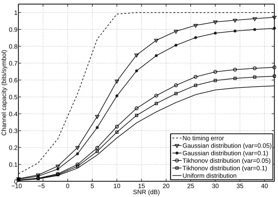
Fig. 2 shows the effect of the timing error on the channel capacity of the DS-BPSK system
in an AWGN channel for different distributions of the timing error. We set Nc = 6. In addition
to the uniform distribution and the Gaussian distribution, the typical Tikhonov distribution for
timing error is also used [35], [36]. One sees that the timing error causes significant performance
degradation to the channel capacity. The channel capacity is the lowest for uniformly distributed
timing error, while the highest for Gaussian distributed timing error. This is due to the fact
that the kurtosis of the Gaussian distribution is the largest while the kurtosis of the uniform
distribution is the smallest, and higher kurtosis gives timing error closer to zero which results in
a stronger signal component. Most well-designed synchronizers follow an asymptotic Gaussian
distribution when the sample size is large [37]. Note that, in practice, the timing error distribution
is implementation dependent and thus we cannot control the distribution.
Fig. 3 shows the effect of the number of users on the channel capacity per user for the
DS-BPSK system in an AWGN channel. Both analytical and simulation results are presented. We
set Nc = 10 and SN R = 6 dB, and the number of users starts from 10. One sees that the
analytical results are very close to the simulation results in all the cases. Comparing channel
capacity for different timing error distributions, one sees that there is a capacity loss of 76%
when the number of users increases from 10 to 100 and timing error is Gaussian distributed,
while there are capacity losses of 77% and 80%, respectively, for Tikhonov distributed timing
error and uniformly distributed timing error. This is because the signal component in the output
of the correlator is stronger for the Gaussian distribution than for the Tikhonov distribution and
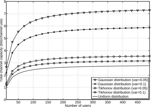
the uniform distribution. Fig. 4 shows the total channel capacity of the same system for all
capacity while the uniform distribution has the lowest total capacity. Moreover, the total capacity
increases with a decrease of variance in the Gaussian distribution.
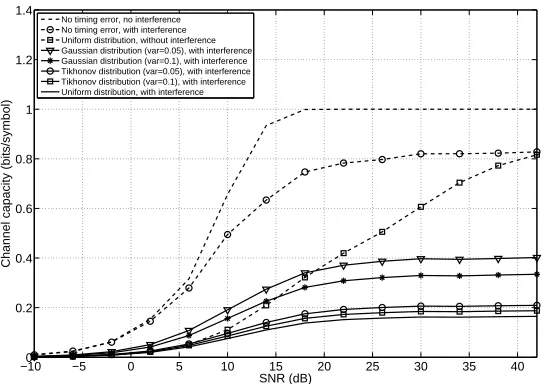
Fig. 5 shows the effect of the interferences and the timing error on the channel capacity of the
DS-BPSK system in the multipath fading channel with a single user. The CM1 channel model is
used. The SNR increases from −10dB to 42dB. We setNc = 6. Simulation results for uniform
distributed timing error are also presented, and it is seen that our semi-analytical results are close
to the simulation results. One also sees that both the timing error and the interferences cause
significant degradation in the channel capacity. Analogous to [18], [19] and [28], the channel
capacity in the multipath fading channel is lower than that in the AWGN channel, under the same
conditions. Comparing the effect of the timing error on the channel capacities for the multipath
fading channel and the AWGN channel, one sees that the detrimental effect of the timing error
is more severe in the multipath fading channel than in the AWGN channel. Therefore, it is more
important to achieve accurate synchronization for the DS-BPSK system in the multipath fading
channel than in the AWGN channel. For the same system, Fig. 6 shows the channel capacity in
the CM2 channel model. Comparing the channel capacity in CM2 with that in CM1, one sees
that the channel capacity in the CM1 channel model is slightly higher than that in the CM2
channel model, under the same conditions. In addition, it is seen that the interferences have
more significant effects on the channel capacity in the CM2 channel model than that in the CM1
channel model. For example, at 0.8 bits/symbol, CM1 has a loss of 9 dB due to interferences
while CM2 has a loss of 15 dB. This is expected. The CM2 channel model does not have a
line-of-sight and the interferences caused by multipath components are stronger in CM2 than
those in CM1.
Fig. 7 shows the total channel capacity in the CM1 channel model. We set SN R = 6 dB
and Nc = 10. The number of users increases from 10 to 490. One sees that the total channel
capacity in the multipath fading channel has similar behaviors to those in the AWGN channel.
Also, the total channel capacity in the multipath fading channel is lower than that in the AWGN
less sensitive to the timing error or its capacity is larger than the DS-BPSK due to the low duty
of cycle with less interferences in this case.
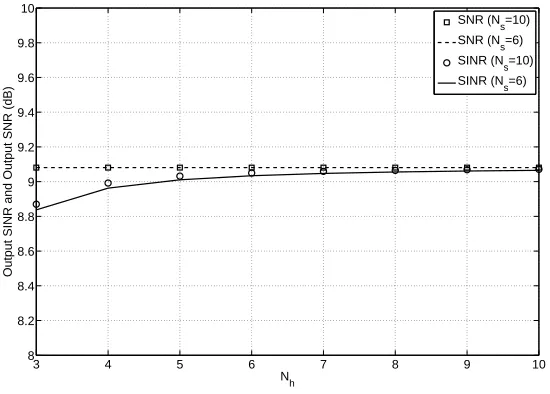
Fig. 8 examines the effect of I on the output SINR of the TH-BPSK system in a single user
AWGN channel for different values ofNs. The value ofNh increases from3to10. The value of
input SNR represents the transmitted signal strength and is set at 18 dB so that the noise is not
dominant and the impact ofI on the output SINR can be clearly observed. It is assumed that the
timing error is uniformly distributed as this is the worst case. The output SNR is around 9.1 dB,
which represents the received signal strength averaged over the timing error and it is different
from the input SNR set at 18 dB as the transmitted signal strength. One sees that the difference
between the output SNR and the output SINR for the same value of Ns decreases when Nh
increases, in all the cases considered. This implies that the value of I is negligible when Nh
is large, because the only difference between SNR and SINR is the value of I. Furthermore,
comparing the difference between the output SNR and the output SINR when Ns = 6 with
that when Ns = 10, one sees that a larger value of Ns results in a smaller difference. This
indicates that the value of I decreases when Ns increases. Consequently, I can be ignored in
the TH-BPSK system when the values of Nh and Ns are large, mainly due to the low duty of
cycle. The ISI depends on the frame duration but Tf =NhTc and Tc is fixed in Fig. 8, so the
effect of Tf is the same as Nh.
Fig. 9 shows the relationship between the number of users and the channel capacity per user
for the TH-BPSK system over AWGN channels. We set Ns = 6 and the SNR is 6 dB. Both
analytical and simulation results are presented. One sees that the analytical results track the
trends of the simulation results well and that the approximation error is small for small values
of the number of users. However, in general, the approximation error is large due to the lower
duty of cycle [38]. Also, one sees that a larger value of Nh results in a larger channel capacity.
Therefore, the capacity loss caused by the MAI or the timing error can be reduced by increasing
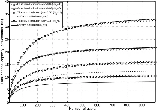
Nh. For the same system, Fig. 10 shows the relationship between the number of users and the
distribution is, the larger the increment of the total channel capacity will be. One sees that a
larger Nh results in a higher increment.
Fig. 11 compares the effect of the interferences and the timing error with different distributions
on the channel capacity of the TH-BPSK system in the CM1 channel model. We set Ns = 6
and Nh = 6. The SNR increases from −10 dB to 42 dB. Simulation results for uniformly
distributed timing error are also presented. It is observed that our semi-analytical results are
close to the simulation results when the SNR is small while there are approximation errors
when the SNR is large. Similar to the channel capacity of the DS-BPSK system, one sees that
both the interferences and the timing error cause significant effects on the channel capacity. As
well, when the timing error and interferences are present, the channel capacity of the TH-BPSK
system in the multipath fading channel approaches an upper limit when the SNR is large. The
processing gain of DS-BPSK in Fig. 5 equals Nc = 6, which is the same as the processing gain
Ns = 6 of BPSK in Fig. 11. Compared with DS-BPSK in Fig. 5, one also sees that
TH-BPSK has higher capacity for the same SNR value and the same timing error distribution. This
is because time-hopping incurs less interferences than direct-sequence due to its very low duty
of cycle such that capacity degradation from interterences is also reduced. For the same system,
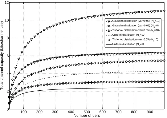
Fig. 12 shows the relationship between the number of users and the total channel capacity in
the CM1 channel model. We set SN R= 6 dB. Again, TH-BPSK has higher total capacity and
can accommodate more users than DS-BPSK system.
The numerical results have illustrated the impact of the number of users on both the channel
capacity and the total channel capacity. This can be used by engineers to design a multiple access
strategy by setting an upper limit for the number of users with maximum total channel capacity
while minimizing the impact of the MAI on the channel capacity for each user. The result in this
paper can be easily extended to binary PPM UWB systems by changing the modulation format
in the signal models. The analysis method is similar, but some conclusions might be different
as PPM has a lower duty of cycle. The result in this paper assumes the Gaussian approximation
exist for small Nu and small Ns but Gaussian approximation is valid for large Nu and Ns in
[39] and [40], in dense multipath even for single user with small Ns [40], [41], as well as for
DS systems and TH systems with large numbers of interfering users [38]. It was also reported
in [42] that a Laplacian approximation to the IPI, ICI and ISI gives better accuracy than the
Gaussian appproximation for large SNRs while they have similar accuracy when the SNR is
less than 10 dB. When the MAI, IPI, ICI and ISI are modeled as non-Gaussian distributions,
such as a Laplacian distribution, the accuracy of the capacity analysis may be improved by
replacing the Gaussian Q function in (8), (22) and (31) with other corresponding functions,
such as a mixture of Gaussian-Q functions [42]. Due to the similarity of the analysis, they are
not presented here. Reference [5] performed a statistical analysis of the interference powers for
DS-BPSK in multipath fading without timing error, while this paper uses a similar method for
both DS-BPSK and TH-BPSK in AWGN and multipath fading with timing error. None of the
results in this paper are the same as those in [5].
Note that the above analysis considers hard-output capacity based on (9) instead of
soft-output capacity. First, the work is presented as a much more complete analysis than [8]- [20]
that used hard-output capacity. Thus, it uses the same capacity definition to facilitate comparison
if one wants. Second, by using (9), one has a direct relationship between capacity and error rate.
Third, unlike the soft-output capacity that only considers the propagation channel, the hard-output
capacity considers the whole system by including modulation and demodulation as part of the
equivalent channel. It is well known that for systems with large operating bandwidths, such as
UWB systems, the soft-output capacity may not be a proper metric, as they only consider the
propagation channel [43], while hard-output capacity takes the whole system into account and
therefore, is more useful in this case. It is very challenging to derive the soft-output capacity and
APPENDIXA
CALCULATION OFE{S2|ǫ}, E{I2|ǫ}ANDE{M AI(k) u
2 }
In this appendix, we calculate E{S2|ǫ}, E{I2|ǫ} and E{M AIu(k) 2
}.
From (5), E{S2|ǫ}=A2E2
gNs2R2g(ǫ). From (6), one has
E{I2|ǫ}=A2Eg2R2g(Tc −ǫ)E{1 +{ Nc−2
X
n=0
βnβn+1}2}. (38)
Since E{{PNc−2
n=0 βnβn+1}2}=Nc−1, one has
E{I2|ǫ}=NcA2Eg2R2g(Tc−ǫ). (39)
Also, from (7), one can have
E{M AI(k) u
2
} = Eg2A(k)2E{
∞
X
m1=−∞
∞
X
m2=−∞
Nc−1 X
n1=0
Nc−1 X
n2=0
Nc−1 X
n′
1=0
Ncs−1 X
n′
2=0
b(k) m1b
(k) m2
βn(k1)β
(k)
n2βn′1βn′2 ·Rg((m1−m˜)Tb+ (n1−n
′
1)Tc +τ(k)−τˆ)
·Rg((m2−m˜)Tb+ (n2−n′2)Tc +τ(k)−τˆ)}. (40)
Since E{b(mk1)b
(k)
m2} = 0 for m1 6= m2, E{β
(k) n1β
(k)
n2 } = 0 for n1 6= n2 and E{βn′1βn′2} = 0 for
n′
1 6=n′2, it can be derived that
E{M AIu(k) 2
}=Eg2A( k)2
∞
X
m=−∞
Nc−1 X
n=0 Nc−1
X
n′=0
E{R2g(Tmm˜ +Tnn′ +τ(k)−τˆ)}, (41)
where Tmm˜ = (m−m˜)Tb and Tnn′(n−n′)Tc. Define
ξmmnn˜ ′ =Tmm˜ +Tnn′ +τ(k)−τ .ˆ
Since ǫ(k) = τ(k) − τˆ is uniformly distributed over a symbol interval, ξ
mmnn˜ ′ is uniformly
distributed over[Tmm˜ +Tnn′, Tmm˜+Tnn′+Tb]. For convenience,ξmmnn˜ ′ is simplified to ξ. When
the second-order derivative Gaussian pulse is used, E{R2
g(ξ)} can be derived as
E{R2g(ξ)} = 1
E2 g
E{ 9
256exp(−8πξ 2/D2
g)− 9πξ2
8D2 g
exp(−8πξ2/Dg2) (42)
+12π 2ξ4 8D4
g
exp(−8πξ2/D2g) + 9π 2ξ4
D4 g
exp(−8πξ2/D2g)
−24π 3ξ6
D6 g
exp(−8πξ2/D2g) + 16π 4ξ8
D8 g
After some simple but tedious mathematical manipulations, every term on the right side of (42)
can be solved. Then, E{M AIu(k) 2
} can be calculated.
REFERENCES
[1] M. Win and R. Scholtz, “Impulse radio: how it works,”IEEE Commun. Lett., vol. 2, pp. 36-38, Feb. 1998.
[2] S. Roy, J. R. Foerster, V. S. Somayazulu and D. G. Leeper, “Ultra-wideband radio design: The promise of high-speed, short-range wireless connectivity,” Invited Paper,Proc. IEEE, vol. 92, no. 2, pp. 295-311, Feb. 2004.
[3] L. Zhao, A. M. Haimovich, “Performance of ultra-wideband communications in the presence of interference,”IEEE J. Select. Areas Commun., vol. 20, no. 9, pp. 1684-1691, Dec. 2002.
[4] Y. Chen and N. C. Beaulieu, “SNR estimation methods for UWB systems,”IEEE Trans. Wireless Commun., vol. 6, pp. 3836-3845, Oct. 2007.
[5] B. Zhao, Y. Chen and R. J. Green, “Average SINR analysis of DS-BPSK UWB systems with IPI, ICI, ISI, MAI and its application,”IEEE Trans. Veh. Technol., vol. 58, no. 8, pp. 4690-4696, Oct. 2009.
[6] T. Jia and D.I. Kim, “Analysis of channel-averaged SINR for indoor UWB rake and transmitted reference systems,”IEEE Trans. Commun., vol. 55, no. 10, pp. 2022-2032, Oct. 2007.
[7] S. Dolinar, D. Divsalar, J. Hamkins and F. Pollara, “Capacity of PPM on Gaussian and Webb channels,”JPL TMO Progress Report, vol. 42-142, pp. 1-31, Apr.-Jun. 2000.
[8] L. Zhao, A. M. Haimovich, “Capacity of M-ary PPM ultra-wideband communications over AWGN channels,”Proceedings of VTC 2001 fall, Oct. 7-11 2001, Altlantic City, New Jersey.
[9] M. Abdel-Hafez, F. Alagöz, M. Hämäläinen and M. Latva-Aho, “On UWB capacity with respect to different pulse waveforms,”WOCN 2005. Second IFIP International Conference, pp. 107-111, Mar. 2005.
[10] J. Zhang, R. A. Kennedy and T. D. Abhayapala, “New results on the capacity of M-ary PPM ultra- wideband systems,” IEEE International Conf. on Communications (ICC), vol. 4, pp. 2867-2871, May 2003.
[11] L. Zhao, A. M. Haimovich, “The capacity of an UWB multi-access communications system,”IEEE International Conf. on Communications (ICC), vol. 3, pp. 1964-1968, 28 Apr. - 2 May 2002.
[12] L. Zhao, A. M. Haimovich, “Multi-user capacity of M-ary PPM ultra-wideband communications,”Proc. IEEE Conf. Ultra Wideband Systems, Technologies, pp.175-179, May 20-23 2002, Baltimore, MD.
[13] A. Adinoyi and H. Yanikomeroglu, “Practical capacity calculation for time-hopping ultra-wide band multiple-access communications,”IEEE Commun. Lett., vol.9, no.7, pp.601-603, Jul. 2005.
[14] H. Zhang and T. A. Gulliver, “Performance and capacity of PAM and PPM UWB time-hopping multiple access communications with receiver diversity,”EURASIP J. Applied Signal Proc., vol. 2005, no. 3, pp. 306-315, Mar. 2005. [15] R. Pasand, S. Khaleshosseini, J. Nielsen and A. Sesay, “The capacity of asynchronous M-ary time hopping PPM UWB
[16] R. Pasand, S. Khaleshosseini and J. Nielsen, “Performance analysis of synchronous M-ary time-hopping PPM UWB multiple-access communication systems,”CCECE/CCGEI. 2005, pp. 1212-1216, May 2005.
[17] M. Abdel-Hafez and F. Alagäz, “Capacity of DS-CDMA versus TH-PPM for multi-user ultra-wideband systems,”IEEE International Symposium on Personal, Indoor and Mobile Radio Communication (PIMRC’06), pp. 1-5, Sept. 2006.
[18] F. Ramirez-Mireles, “On the capacity of UWB over multipath channels,”IEEE Commun. Lett., vol. 9, no. 6, pp. 523-525, Jun. 2005.
[19] T. Erseghe, “Capacity of UWB impulse radio with single-user reception in Gaussian noise and dense multipath,” IEEE Trans. Commun., vol. 53, no. 8, pp. 1257-1262, Aug. 2005.
[20] N. Güney, H. Delic˛, and F. Alagöz, “Achievable information rates of M-ary PPM impulse radio for UWB channels and Rake reception,”IEEE Trans. Commun., vol. 58, no. 5, pp. 1524-1535, May 2010.
[21] F. Ramirez-Mireles, “Performance of UWB N-Orthogonal PPM in AWGN and multipath channels” IEEE Trans. Veh. Technol., vol. 56, no. 3, pp. 1272-1285, May 2007.
[22] Y. Chen and N.C. Beaulieu “Interference analysis of UWB systems for IEEE channel models using first- and second-order moments,”IEEE Trans. Commun., vol. 57, no. 3, pp. 622-625, Mar. 2009.
[23] Z. Tian and G. B. Giannakis, “BER sensitivity to mistiming in Ultra-Wideband impulse radios - Part I: nonrandom channels,”IEEE Trans. on Signal Proc., vol. 53, no. 4, pp. 1550-1560, Apr. 2005.
[24] N. V. Kokkalis, P. T. Mathiopoulos, G. K. Karagiannidis and C. S. Koukourlis, “Performance analysis of M-ary PPM TH-UWB systems in the presence of MUI and timing jitter,”IEEE J. Select. Areas Commun., vol. 24, no. 4, pp. 822-828, Apr. 2006.
[25] S. Gezici, A. F. Molisch, H. V. Poor and H. Kobayashi “The tradeoff between processing gains of an impulse radio UWB system in the presence of timing jitter,”IEEE Trans. Commun., vol. 55, no. 8, pp. 1504-1511, Aug. 2007.
[26] M. Kamoun, M. Courville, L. Mazet and P. Duhamel, “Impact of desynchronization on PPM UWB systems: a capacity based approach,”IEEE Information Theory Workshop 2004, pp. 198-203, 24-29 Oct. 2004.
[27] B. Hu and N. C. Beaulieu, “Exact bit error rate analysis of TH-PPM UWB systems in the presence of multiple access interference,”IEEE Commun. Lett., vol. 7, no. 12, pp. 572-574, Dec. 2003.
[28] F. Ramirez-Mireles, "Quantifying the degradation of combined MUI and multipath effects in impulse-radio UWB,"IEEE Trans. on Wireless Commun., vol. 6, pp. 2831-2836, Aug. 2007.
[29] R. Knopp, P.A. Humblet, "Information capacity and power control in single-cell multiuser communications,"Proc. IEEE ICC 1995, vol. 1, pp. 331-335, Seattle, USA, 1995.
[30] B. Hu and N. C. Beaulieu, “Accurate performance evaluation of time-hopping and direct-sequence UWB systems in multi-user interference,”IEEE Trans. Commun., vol. 53, no. 6, pp. 1053-1062, Jun. 2005.
[31] J. G. Proakis,Digital Communication, 3rd ed. London, U.K.: McGraw-Hill, 1995. [32] “Channel modeling sub-committee report final,” IEEE P802.15-02/368r5-SG3a, Dec. 2002.
[34] B. Hu and N. C. Beaulieu, “Pulse shapes for Ultrawideband communication systems,”IEEE Trans. Wireless Commun., vol. 4, no. 4, pp. 1789-1797, Jul. 2005.
[35] M. Moeneclaey, “The influence of four types of symbol synchronizers on the error probability of a PAM receiver,”IEEE Trans. Commun., vol. 32, no. 11, pp. 1186-1190, Nov. 1984.
[36] K. Bucket and M. Moeneclaey, “Effect of random carrier phase and timing errors on the detection of narrowband M-PSK and bandlimited DS/SS M-PSK signals,”IEEE Trans. Commun., vol. 43, no. 2/3/4, pp. 1260-1263, Feb.-Mar.-Apr. 1995. [37] U. Mengali and A. N. D’Andrea,Synchronization Techniques for Digital Receivers, New York, Plenum Press, 1997. [38] N. C. Beaulieu and D. J. Young, “Designing time-hopping ultra-wide bandwidth receivers for multi-user interference
environments,” Invited Paper,Proc. IEEE, vol. 97, no. 2, pp. 255-283, Feb. 2009.
[39] Y. Dhibi and T. Kaiser, “On the impulsiveness of multiuser interferences in TH-PPM-UWB systems,” IEEE Trans. on Signal Proc., vol. 54, no. 7, pp. 2853-2857, Jul. 2006.
[40] F. Ramirez-Mireles and A. Almada, “Testing the Gaussianity of UWB TH-PPM MUI with imperfect power control and multipath,”Proc. 5th International Conf. on Electrical Engineering, Computing Science and Automatic Control, ,pp. 242-247, 12-14 Nov. 2008.
[41] Q.T. Zhang and S.H. Song, “Parsimonious correlated nonstationary models for real baseband UWB data",IEEE Trans. on Veh. Technol., vol. 54, pp. 447-455, Mar. 2005.
[42] H. Shao and N.C. Beaulieu, "An analytical method for calculating the bit error rate performance of Rake reception in UWB multipath fading channes,"Proc. ICC 2008, pp. 4855-4860, Beijing, China, May 2008.
−100 −5 0 5 10 15 20 25 30 35 40 0.1
0.2 0.3 0.4 0.5 0.6 0.7 0.8 0.9 1
SNR (dB)
Channel capacity (bits/symbol)
TH System with Rectangular Pulse
TH System with the 2nd−order derivative Gaussian pulse TH System with the 4th−order derivative Gaussian pulse DS System with Rectangular pulse
[image:23.595.170.441.148.343.2]DS System with the 2nd−order derivative Gaussian pulse DS System with the 4th−order derivative Gaussian pulse
Fig. 1. Channel capacity v.s. SNR for different pulse shapes in DS-BPSK and TH-BPSK systems
with a single user over AWGN channels. The timing error is uniformly distributed.
−100 −5 0 5 10 15 20 25 30 35 40 0.1
0.2 0.3 0.4 0.5 0.6 0.7 0.8 0.9 1
SNR (dB)
Channel capacity (bits/symbol)
No timing error
Gaussian distribution (var=0.05) Gaussian distribution (var=0.1) Tikhonov distribution (var=0.05) Tikhonov distribution (var=0.1) Uniform distribution
Fig. 2. Channel capacity v.s. SNR for the DS-BPSK system with/without timing error in an
[image:23.595.168.441.474.667.2]10 20 30 40 50 60 70 80 90 100 0
0.05 0.1 0.15 0.2 0.25 0.3 0.35
Number of users
Channel capacity (bits/symbol)
[image:24.595.165.444.137.331.2]Analytical result, Gaussian distribution (var=0.05) Simulation, Gaussian distribution (var=0.05) Analytical result, Tikhonov distribution (var=0.05) Simulation, Tikhonov distribution (var=0.05) Analytical result, uniform distribution Simulation, uniform distribution
Fig. 3. Channel capacity per user v.s. the number of users for the DS-BPSK system with different
timing error distributions in an AWGN channel. The second-order derivative Gaussian pulse is
used.
50 100 150 200 250 300 350 400 450 0
1 2 3 4 5 6 7 8
Number of users
Total channel capacity (bits/channel use) Gaussian distribution (var=0.05)
Gaussian distribution (var=0.1) Tikhonov distribution (var=0.05) Tikhonov distribution (var=0.1) Uniform distribution
Fig. 4. Total channel capacity for all users v.s. the number of users for the DS-BPSK system with
different timing error distributions in an AWGN channel. The second-order derivative Gaussian
[image:24.595.175.440.463.652.2]−100 −5 0 5 10 15 20 25 30 35 40 0.2
0.4 0.6 0.8 1 1.2 1.4
SNR (dB)
Channel capacity (bits/symbol)
[image:25.595.169.443.147.342.2]No timing error, no interference No timing error, with interference Uniform distribution, without interference Gaussian distribution (var=0.05), with interference Gaussian distribution (var=0.1), with interference Tikhonov distribution (var=0.05), with interference Tikhonov distribution (var=0.1), with interference Uniform distribution, with interference Simulation, uniform distribution, with interference
Fig. 5. Channel capacity v.s. SNR for the DS-BPSK system with/without the interferences and
the timing error in the CM1 channel model. The second-order derivative Gaussian pulse is used.
−100 −5 0 5 10 15 20 25 30 35 40 0.2
0.4 0.6 0.8 1 1.2 1.4
SNR (dB)
Channel capacity (bits/symbol)
No timing error, no interference No timing error, with interference Uniform distribution, without interference Gaussian distribution (var=0.05), with interference Gaussian distribution (var=0.1), with interference Tikhonov distribution (var=0.05), with interference Tikhonov distribution (var=0.1), with interference Uniform distribution, with interference
Fig. 6. Channel capacity v.s. SNR for the DS-BPSK system with/without the interferences and
[image:25.595.169.441.473.665.2]50 100 150 200 250 300 350 400 450 0
1 2 3 4 5 6 7
Number of users
Total channel capacity (bits/channel use)
[image:26.595.173.440.141.331.2]TH System with Gaussian Distributed Timing Errors (var=0.05) TH System with Tikhonov Distributed Timing Errors (var=0.05) DS System with Gaussian Distributed Timing Errors (var=0.05) TH System with Uniform Distributed Timing Errors DS System with Tikhonov Distributed Timing Errors (var=0.05) DS System with Uniform Distributed Timing Errors
Fig. 7. Total channel capacity v.s. the number of users for the DS-BPSK and TH-BPSK systems
with different timing error distributions in the CM1 channel model. The second-order derivative
Gaussian pulse is used.
3 4 5 6 7 8 9 10
8 8.2 8.4 8.6 8.8 9 9.2 9.4 9.6 9.8 10
Nh
Output SINR and Output SNR (dB)
SNR (Ns=10) SNR (Ns=6) SINR (Ns=10) SINR (Ns=6)
Fig. 8. Output SINR and output SNR v.s. Nh for the TH-BPSK system in an AWGN channel.
[image:26.595.168.443.480.677.2]10 20 30 40 50 60 70 80 90 100 0
0.05 0.1 0.15 0.2 0.25 0.3 0.35 0.4 0.45 0.5
Number of users
Channel capacity (bits/symbol)
Analytical result, Gaussian distribution (var=0.05) (N
h=10)
Simulation, Gaussian distribution (var=0.05) (Nh=10) Analytical result, Gaussian distribution (var=0.05) (Nh=6) Simulation, Gaussian distribution (var=0.05) (Nh=6) Analytical result, uniform distribution (Nh=10) Simulation, uniform distribution (Nh=10) Analytical result, uniform distribution (Nh=6) Simulation, uniform distribution (N
[image:27.595.166.443.136.332.2]h=6)
Fig. 9. Channel capacity per user v.s. the number of users for the TH-BPSK system with different
timing error distributions in an AWGN channel. The second-order derivative Gaussian pulse is
used.
100 200 300 400 500 600 700 800 900 0
5 10 15 20 25 30 35 40
Number of users
Total channel capacity (bits/channel use)
Gaussian distribution (var=0.05) (Nh=10) Gaussian distribution (var=0.05) (N
h=6)
Tikhonov distribution (var=0.05) (Nh=10) Uniform distribution (Nh=10) Tikhonov distribution (var=0.05) (Nh=6) Uniform distribution (Nh=6)
Fig. 10. Total channel capacity for all users v.s. the number of users for the TH-BPSK system with
different timing error distributions in an AWGN channel. The second-order derivative Gaussian
[image:27.595.170.442.463.652.2]−100 −5 0 5 10 15 20 25 30 35 40 0.2
0.4 0.6 0.8 1 1.2 1.4
SNR (dB)
Channel capacity (bits/symbol)
[image:28.595.169.441.141.335.2]No timing error, no interference No timing error, with interference Uniform distribution, without interference Gaussian distribution (var=0.05), with interference Gaussian distribution (var=0.1), with interference Tikhonov distribution (var=0.05), with interference Tikhonov distribution (var=0.1), with interference Uniform distribution, with interference Simulation, uniform distribution, with interference
Fig. 11. Channel capacity v.s. SNR for the TH-BPSK system with/without the interferences and
the timing error in the CM1 channel model. The second-order derivative Gaussian pulse is used.
100 200 300 400 500 600 700 800 900 0
2 4 6 8 10 12
Number of uers
Total channel capacity (bits/channel use)
Gaussian distribution (var=0.05) (N
h=10)
Gaussian distribution (var=0.05) (Nh=6) Tikhonov distribution (var=0.05) (Nh=10) Uniform distribution (N
h=10)
Tikhonov distribution (var=0.05) (Nh=6) Uniform distribution (Nh=6)
Fig. 12. Total channel capacity v.s. the number of users for the TH-BPSK system with different
timing error distributions in the CM1 channel model. The second-order derivative Gaussian pulse
[image:28.595.171.442.458.650.2]