a Corresponding author: [email protected]
Numerical simulation and experimental visualization of the separated
cavitating boundary layer over NACA2412
Jiří Kozák 1,a, Pavel Rudolf1, Milan Sedlář2, Vladimír Habán1, Martin Hudec1and Rostislav Huzlík3
1 Victor Kaplan Dept. of Fluid Engineering, Faculty of Mechanical Engineering, Brno University of Technology, Czech Republic
2 Centre of Hydraulic Research, J. Sigmunda 190, Lutín, Czech Republic
3 Faculty of Electrical Engineering and Communications, Brno University of technology, Czech Republic
Abstract.Cavitation is physical phenomenon of crucial impact on the operation range and service lifetime of the hydraulic machines (pumps, turbines, valves etc.). Experimental measurement of cavitation is expensive and time consuming process, while some important characteristic of the flow are difficult to measure due to the nature of the phenomenon. Current possibilities of computational fluid dynamics provide a way for deeper understanding of cavitation which is important for many applications in the hydraulic machines industry such as expanding operation range or extending lifetime of the hydraulic machines. Simplified model consists of NACA 2412 hydrofoil with 8 degrees angle of attack fixed in between the walls of cavitation tunnel. Present investigation focuses on comparison of vapor volume fractions obtained by 3D CFD simulations and high speed visualization of the real cavitation phenomena. Several operating regimes corresponding to different cavitation numbers are studied with aim to assess the dynamics of the separated cavitating sheets/clouds
1. Introduction
Cavitation is physical phenomenon of vapor phase creation in liquid flow caused by pressure reduction at constant ambient temperature. Since the cavity filled with vapor is still part of the flow it is convected downstream to a region of higher pressure, where cavity collapses. Specific volume of vapor is higher than specific volume liquid, therefore the inception and collapse of cavity is accompanied by emission of pressure shocks and acoustic waves. Moreover, in case of wall presence in the area of collapsing cavities the rapid wear of surfaces called erosion occurs, while the wear of the surfaces of the hydrofoil is highly influenced by the unsteady cloud shedding. [1]
Cavitation phenomenon could be characterized by the dimensionless cavitation number σ.
σ = p∞ - pv
0.5ρv∞2 (1)
Where p∞ and v∞ are free stream pressure and velocity, ρ is density of the liquid and pv is pressure of saturated vapor. It should be mentioned that computation of cavitation number was based on the characteristics of the flow in the inlet section of the test part of cavitation tunnel (rectangular shape).
Cavitation over hydrofoil is typical example of hydrodynamic cavitation, where the pressure drop is induced by local flow speed up in the area of the suction side of the hydrofoil. In fact, this simple geometry could be used for study of cavitation in hydraulic facilities such
as turbines and pumps where the complex machine geometry makes the experimental and computational investigation of cavitation structures very difficult.
The interaction of the separated flow and cavitation leads to a complex flow, which is still quite challenging to be simulated correctly due to its physical complexity and dynamic behaviour.
This contribution is focused on numerical simulation of unsteady cavitating flow around NACA 2412. The results of full 3D simulation are compared with the experimental data in the main part of the work from the viewpoint of separated cavitating sheets/clouds dynamics.
2. Cavitation cloud separation
The vapor cavity is stable in case of higher values of cavitation number σ. In that cases only the thin cavities are created, therefore the backflow behind the cavity could be re-entrained locally and influence of the backflow is not so important. This configuration leads to the stable behaviour of the flow.
The thickness of the vapor cavity grows with the decreasing value of cavitation number. Importance of the backflow influence grows rapidly in this case.
The flow rate of the counter flow is higher than in case of higher values of cavitation number which leads to creation of so-called re-entrant jet. Re-entrant jet is unstable region of counter flow attached to the hydrofoil surface. The presence of the re-entrant jet leads to the separation of the cavity from the surface of the hydrofoil. DOI: 10.1051/
C
Owned by the authors, published by EDP Sciences, 2015
/201 020
epjconf EPJ Web of Conferences ,
020 59 92
2 3
3 (2015)
7
As the region of re-entrant jet grows toward the leading edge of the hydrofoil, part of the cavity is separated. The separated cavitation cloud is entrained downstream by the main flow to the region of higher pressure and above described cycle of re-entrant jet forming and separation of the cavitation cloud repeats. The typical cycle of cavity inception and separation of the cavitation cloud is depicted in the following picture.
Figure 1 Shedding cycle
3. Experimental set-up
The experimental part of the work was carried out in the Centre of Hydraulic Research which is equipped with the horizontal cavitation tunnel. The different static pressure levels were set up with compressor and vacuum pumps. The NACA 2412 hydrofoil, manufactured from aluminium, was fixed between the walls of the rectangular (150 x 150 mm) part of the cavitation tunnel with the 8 degrees incidence angle. The chord length of the investigated prismatic hydrofoil was
120 mm. The span/chord length ratio influences the shape of shedding cavities. Value of span/chord ratio is 1.25 in this case, therefore it can be assumed that the flow near the midspan of the hydrofoil was not highly influenced by the presence of the walls of cavitation tunnel. [2]
The static pressure was recorded with two midspan pressure transducers. First of them was situated on the leading edge, the second transducer was placed in the 40 % of the chord length. The sampling frequency of the transducers was 5 kHz. The accuracy of the pressure transducers was 0.5 kPa. The flowmeter accuracy was 3.5 l/s.
The walls of the cavitating tunnel were manufactured from transparent organic glass, which allowed visualization of cavitating flow with high speed cameras.
Sampling frequency of the top camera was 3 kHz while the frequency of the side camera was approximately ten times lower.
The cavitating flow was captured from the top and from the side of the hydrofoil simultaneously when the video was synchronized with transducers through the voltage marker signal.
This experimental set-up allows obtaining complex information about dynamics of the cavitating flow, which is necessary for the further verification of the numerical results.
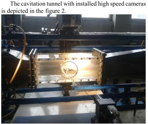
The cavitation tunnel with installed high speed cameras is depicted in the figure 2.
Figure 2 Cavitation tunnel with the high speed cameras
4. Computational mesh and numerical
set-up
The geometry of the cavitation tunnel with NACA 2412 hydrofoil was decomposed and meshed in software Gambit. Besides the main rectangular part of the cavitation tunnel with the hydrofoil, the upstream and downstream reducers with certain length of the pipes (3 diameters on the inlet and nearly 4 diameters on the outlet of the computational domain) were included in the computational domain.
The structured computational mesh consisted of approximately 2.5 million of hexahedral cells. The regions of boundary layers near the walls of hydrofoil and cavitation tunnel were refined in order to reach correct value of the y+ for the purpose of the near-wall treatment.
The cells with the worst quality were situated behind the trailing edge where the value of aspect ratio exceeded value of 150. Moreover, the necessity of keeping value of aspect ratio within reasonable limits in the area of vapor cavity inception near the leading edge of the hydrofoil has arrised. In the case that poor quality cells were located in this area the stability of the simulation dramatically decreased.
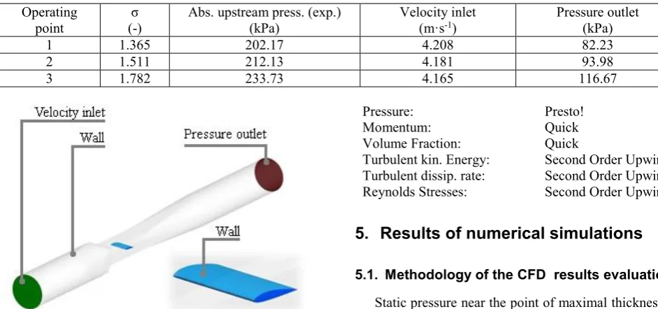
Boundary conditions were chosen as follows:
x Inlet of computational domain: velocity inlet x Outlet of computational domain: pressure outlet x Surfaces of hydrofoil and tunnel: walls
Figure 3 Computational domain (green - velocity inlet, red pressure outlet, blue - surfaces of NACA 2412 hydrofoil)
Value of inlet velocity was set according to the experimental data. Value of the gauge pressure on the outlet boundary was set so as to obtain experimentally measured pressure in the cross section of the upstream pipe. (Table 1) The numerical simulations were carried out for three operating points with different cavitation number σ.
Values of inlet velocities and outlet pressures used in each of the investigated cases are listed in the table 1.
The ANSYS Fluent 14.5 and 15 (different versions on the different computers) was used for the purpose of cavitating flow numerical simulations. The simulations were carried out as transient with 5E-5 s time step length. The turbulence was modelled using RSM model where the whole tensor of turbulent stresses is computed. This approach should guarantee better result than k-ε model or other two-equation models which are considering isotropic turbulence. [3]
Moreover the damping of the cavitation dynamics is far more significant in case of the k-ε model of turbulence. On the other hand the approach of turbulence modelling is still quite problematic for the purpose of the cavitation shedding dynamics simulation. It is reasonable to predict that better result could be obtained in case of more complex approach such as large eddy simulation (LES) where the Navier-Stokes equations are directly numerically solved for a large part of the spectrum of vortices.
Cavitating flow is example of two phase flow therefore liquid phase, vapor phase and mechanism of phase transition between them need to be specified. The two phase mixture method is considered in this contribution. The mass transfer is modelled using Schnerr-Sauer model, which works with simplified Rayleigh-Plesset equation Simple algorithm is used to solve the set of governing equations. [4]
Complete setting of the chosen discretization schemes is listed in the following chart.
Pressure: Presto!
Momentum: Quick
Volume Fraction: Quick
Turbulent kin. Energy: Second Order Upwind Turbulent dissip. rate: Second Order Upwind Reynolds Stresses: Second Order Upwind
5. Results of numerical simulations
5.1. Methodology of the CFD results evaluation
Static pressure near the point of maximal thickness of hydrofoil was monitored during the computations. The position of the pressure monitor was the same as the position of the transducer during the experiments; therefore the comparison was possible between the experiments and simulations. The value of the static pressure was computed as the vertex average. The vertex average of the static pressure is computed as the average value of the pressure in the cells neighboring to the point of monitor.
The position of the stagnant line (boundary of the re-entrant jet) was compared with the position and shape of the cavity volume in different phases of the cavity inception and separation.
Drag and lift coefficient were evaluated in the previously mentioned phases of the cavity development as an additional information of the cavitation phenomenon influence on the operation of the hydraulic machines.
Further characteristics of the cavitation were visualized through the surface streamlines on the suction side of the hydrofoil.
It should be mentioned that stability of the computation was not ideal in any of the investigated cases, which will be depicted and described in the following chapters. Unfortunately, the instability influenced the results of the computations significantly.
5.2. Pressure fluctuations
The value of the static pressure was evaluated in every timestep in the position of the transducer as it was mentioned in the previous paragraph. Periodic pressure shocks were observed in all of the three investigated operating points. In fact the sudden nature of the pressure pulses made impossible to perform FFT of the pressure fluctuation signal, despite the short length of the transient simulation timestep. Therefore the cavitation cloud separation period was estimated only on the basis of the average time between two pressure peaks.
The amplitudes of the pressure signals are particularly significant in case of operating points 2 and 3 (σ = 1.511 Table 1 Operating points and boundary conditions
Operating point
σ (-)
Abs. upstream press. (exp.) (kPa)
Velocity inlet (m·s-1)
Pressure outlet (kPa)
1 1.365 202.17 4.208 82.23
2 1.511 212.13 4.181 93.98
3 1.782 233.73 4.165 116.67
and 1.782), where the value of maximal pressure exceeds 3 MPa as is shown in the following graphs (blue lines).
Graph 1 OP 1 – period of cloud shedding
Graph 2 OP 2 – period of cloud shedding
Graph 3 OP 3 – period of cloud shedding
Values of the cavitation cloud shedding frequencies (average) and their comparison with the results obtained experimentally are listed in the table 2. It should be mentioned that it was not possible to perform FFT analysis of the pressure signals, due to the sudden character of the pressure peaks.
Therefore the frequencies of the cavitation cloud shedding were estimated from the static pressure course as the reciprocal value of the average period between consecutive pressure peaks in case of CFD computations.
Most significant difference of the experimentally and numerically obtained values of shedding frequency could be found in case of the OP 1, where the difference is equal to 1.6 Hz. In case of OP 2 (respectively OP 3) the difference is approximately half (0.7 Hz and 0.82 Hz).
The graphs of static pressure course during one period of cloud separation are extended by the information about lift/drag coefficient ratio (red line in the graphs 1, 2 and 3). It is noticeable that the maximal value of the ratio shortly precedes the peak of the pressure in all of the investigated operating points. Significant amplitudes of the lift/drag ratio course could be seen for OP 2 and 3 as in the case of the static pressure course.
This behaviour or instability is probably caused by numerical basis of the ANSYS Fluent, therefore only the OP 1 was chosen for the further investigation, despite the fact that the difference of cloud shedding frequency was the most significant.
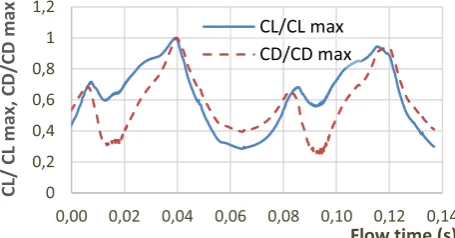
Coefficient of drag and lift course during one period (OP 1) are separately depicted in the graph 4. The values (CFD) of the coefficients are depicted in form of ratio between actual and maximal value of the coefficient. The maximum value of the lift coefficient was 4.83, maximum observed value of the drag coefficient was 1.39.
Graph 4 OP 1- lift and drag coefficient during one period
5.3. Cavitation cloud separation
The phases of the cavity inception and separation were captured through surface of the constant volume fraction of the vapor. Value of 50 % (semitransparent light-blue surface) and 10 % (dark blue surface) vapor fraction were chosen for the purpose of the contribution, while the pictures were captured from the top and from the side of the hydrofoil.
At the beginning of the cloud shedding period there was only a narrow strip of cavitation downstream of the leading edge. Significant difference between simulation and experiment could be found in this part of period. The thickness of the cavitation cloud increased as well as its length. The development of the cavitation cloud was more rapid near the walls of cavitation tunnel therefore the cavitation cloud forms its typical U-shape. Increase of the re-entrant jet influence led to cavitation cloud separation from the surface of the suction side of the hydrofoil. When the length of cavitation clouds reached certain value the extended sides of the cloud got merged so the cloud got nearly rectangular shape with hole in its center (from the top view). In this moment the computationally obtained shape of cavitation cloud meets the experiment quite well. In the last part of the period further growth of cloud was observed. At a certain point, when the cloud reached the region of higher pressure the cloud collapsed which was accompanied with the noticeable pressure shock. It should 0 2 4 6 8 10 -100 -50 0 50 100 150
0,00 0,02 0,04 0,06 0,08 0,10 0,12
CL/CD
Static p
ressur
e (kPa)
Flow time (s)
Static pressurere CL/CD -200 300 800 1300 -100 900 1900 2900 3900 4900
0,00 0,02 0,04 0,06 0,08 0,10 0,12
CL/CD
Static pressur
e
(kPa)
Flow time (s)
Static pressure CL/CD -10 -5 0 5 10 15 -100 900 1900 2900 3900 4900
0,00 0,02 0,04 0,06 0,08 0,10 0,12
CL/CD
Static p
ressur
e (kPa
)
Flow time (s)
Static pressure CL/CD 0 0,2 0,4 0,6 0,8 1 1,2
0,00 0,02 0,04 0,06 0,08 0,10 0,12 0,14
CL/ CL m
ax,
CD/CD
max
Flow time (s) CL/CL max
CD/CD max
OP T (s) f (Hz) f (exp.) (Hz)
1 0.0785 12.74 14.34
2 0.0691 14.48 15.18
3 0.0693 14.44 15.26
be mentioned that another volume of cavitation was observed from time to time behind the trailing edge.
The development of the cavitation cloud is depicted in the following pictures.
t =
0.022
2 s
t =
0.032
2 s
t =
0.042
2 s
t =
0.052
2 s
Table 3 OP 1 Comparison of CFD computation with experiment. Semi-transparent light blue contour – 10 % of vapour fraction, dark blue contour – 50 % vapour fraction. Specified time corresponds to CFD simulation
The direct qualitative comparison of computation and experiments shows, that it is not possible to capture some physical phenomena such as horseshoe vortices which were formed on suction side of hydrofoil from time to
time. It is noticeable that it was not possible to capture full complexity of the cavitating flow using Reynolds stress model of turbulence, which results from the nature of turbulence modelling. From this point of view use of more
t =
0.062
2 s
t =
0.072
2 s
t =
0.082
2 s
t =
0.092
2 s
t =
0.102
complex approach of flow modelling (i.e. LES, DES) seems to be promising. [5][6]
On the other hand LES or DES numerical computations have far greater demands on the quality and near wall refinement of the computational mesh.
Despite the previously mentioned facts it was possible to capture periodic character of the inception, growth and shedding of the cavitation cloud.
The growth of the cloud before its separation is quite slow and covers nearly two-thirds of the period. Collapse of the cloud in the last third of the period is relatively rapid.
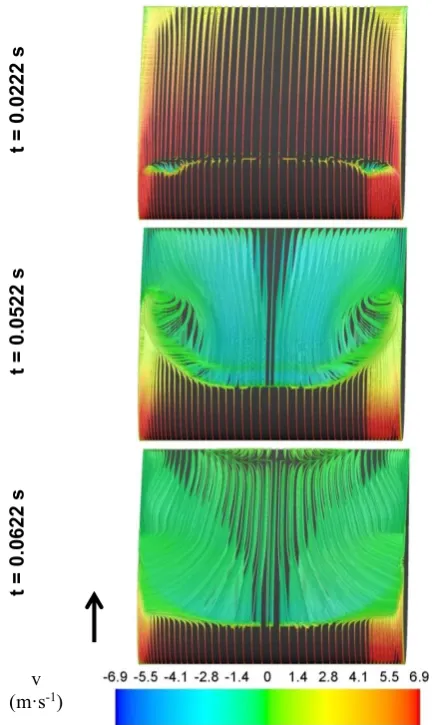
5.4. Re-entrant jet and flow near the hydrofoil surface
The creation and presence of the re-entrant jet has crucial influence on cavitation cloud separation from the surface of hydrofoil as was described in the chapter 2. Therefore, the development of the re-entrant jet was investigated in several phases of the period as well as the flow field near the hydrofoil. The properties of the flow field near the surface of the suction side of hydrofoil were visualized through surface streamlines which were colored by hydrofoil longitudinal component of velocity (figure 4, the value of the velocity is negative in the region of re-entrant jet).
t =
0.022
2 s
t =
0.052
2 s
t =
0.062
2 s
v (m·s-1)
Figure 4 Surface streamlines during one period of cloud separation
The position of the flow separation corresponds to the regions where the streamlines are disconnected in the pictures. Quite interesting is the third picture from the series (t = 0.0622 s) where the second separation of the flow could be found near the trailing edge.
The re-entrant jet and its influence on cavitation cloud shape and behaviour is depicted in the following pictures. The first picture is depicting contours of volume fraction in the midspan slice of the domain at the beginning of the period. The cavitation cloud is thin, therefore the flow could be re-entrained and there is no significant region of the backflow (figures 5 and 6).
Figure 5 Water volume fraction contours with detail of re-entrained flow behind the cavitation cloud. (t = 0.0222 s)
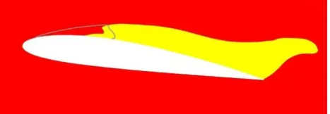
The absence of the re-entrant jet in this phase of cavitation cloud creation is shown in the figure. 6, where only the small area of the backflow could be found in front of the leading edge (the 10 % volume fraction of vapor is marked by the grey line )
Figure 6 Contours of backflow (yellow), only the small region of backflow could be found near the leading. (t = 0.0222 s)
The flow around the hydrofoil has completely different character for the flow time t = 0.0522 s (figures 7 and 8). The contours are complemented with the vectors of the flow velocity. The re-entrant jet is acting against the cavitation cloud near the leading edge. Moreover, there is another region of the significant vapour volume presence behind the trailing edge.
Figure 7 Water volume fraction contours with detail of re-entrant jet and vortices (t = 0.0522 s)
The whole region of backflow is depicted in the following picture together with the border line of the 10%
volume fraction of the water vapour in the midspan slice of the computational domain.
Figure 8 Contours of backflow (yellow), the backflow is developed and covers significant part of suction side of hydrofoil (t = 0.0522 s)
6. Conclusions
The results described in the present contribution confirmed that it could be still quite challenging to simulate dynamics of complex multiphase flow properly. The occurrence of unrealistic severe pressure pulses had been observed in each of three investigated operating points. The less significant pressure pulses were observed in case of the OP 1, therefore this case was described in greater detail. Volume of the cavitation cloud during the period was compared with high-speed video. The most significant difference could be found at the beginning and at the end of the period, while quite good agreement could be found in the vicinity of the cavitation cloud volume peak.
The flow along the suction side of the hydrofoil was depicted through surface streamlines in the different parts of cavitation cloud shedding period. Thus it was possible to capture character of the flow as well as the line of the flow separation compared with the region of back flow.
The frequencies of the cavitation cloud shedding were in good agreement with the experientially obtained data. Unfortunately due to the sudden nature of the pressure pulsation obtained by the numerical simulations it was not possible to do FFT analysis of the signals. Therefore the values were estimated only on the basis of the average period between pressure pulses.
The most important problem would be to remove problem with the stability, therefore different type of boundary conditions or approach to turbulence modelling should be tested.
References
[1] SIROK B., DULAR M. and NOVAK M. et al. The influence of cavitation structures on the erosion of a symmetrical hydrofoil in a cavitation tunnel. Mech. Engineering, pp. 354-361, (2002)
[2] M. Sedlar, M. Komarek, P. Rudolf, J. Kozak, R. Huzlik. Numerical and Experimental Research on
Unsteady Cavitating Flow around NACA 2412
Hydrofoil. International Symposium of Cavitation and multiphase Flow (2014)
[3] GREESHMA P. Rao, LIKITH K., and MOHAMMED N. Akram, et al. Numerical analysis
of cavitating flow over A2d Symmetrical hydrofoil.
International Journal of Computational Engineering Research, Mech. Engineering, pp 1462-1469, (2012)
[4] ANSYS FLUENT 12.0: Theory Guide [online]. c2009 [cit. 10.9.2014]. Available from:
orange.engr.ucdavis.edu/Documentation12.0/120/F LUENT/flth.pdf
[5] BENSOW E. R., Simulation of the unsteady cavitation on the the DELFT TWIST11 foil using RANS, DES and LES. Second International Symposium on Marine Propulsors, (2011)
[6] ROOHI, Ehsan, Amir POUYAN ZAHIRI a Mahmud PASANDIDEH-FARD. Numerical Simulation of Cavitation around a Two-Dimensional Hydrofoil using VOF Method and LES Turbulence Model.
Proceedings of the 8th International Symposium on Cavitation. Singapore: Research Publishing Services, pp. 661-666. DOI: 10.3850/978-981-07-2826-7_141,
(2012) Available from: http://rpsonline.com.sg/proceedings/9789810728267
/html/141.xml3