Model-based Recursive Partitioning
Meets
Item Response Theory
New Statistical Methods for the Detection of
Differential Item Functioning and
Appropriate Anchor Selection
Dissertation
an der Fakult¨at f¨ur Mathematik, Informatik und Statistik
der Ludwig-Maximilians-Universit¨at M¨unchen
vorgelegt von
Julia Kopf
am 14.08.2013
Datum der Einreichung: 14.08.2013
Erstgutachterin: Prof. Dr. Carolin Strobl
Zweitgutachter: Prof. Dr. Thomas Augustin
Drittgutachter: Prof. Dr. Achim Zeileis
Summary
The aim of this thesis is to develop new statistical methods for the evaluation of assumptions that are crucial for reliably assessing group-differences in complex studies in the field of psy-chological and educational testing.
The framework of item response theory (IRT) includes a variety of psychometric models for scaling latent traits such as the widely-used Rasch model. The Rasch model ensures objective measures and fair comparisons between groups of subjects. However, this important property holds only if the underlying assumptions are met. One essential assumption is the invariance property that states constant item parameters for all subgroups. Its violation is extensively discussed in the literature and termed differential item functioning(DIF). This thesis focuses on the methodology of DIF detection. Existing methods for DIF detection are briefly discussed and new statistical methods are introduced.
Zusammenfassung
Ziel dieser Arbeit ist die Entwicklung neuer statistischer Methoden zur ¨Uberpr¨ufung von An-nahmen, die maßgeblich f¨ur die Analyse von Gruppenunterschieden in komplexen Studien aus dem Bereich der Psychologie und der empirischen Bildungsforschung sind.
DieItem Response Theory(IRT) umfasst eine Vielzahl psychometrischer Modelle zur Skalierung
latenter Personeneigenschaften, wie das weit verbreitete Rasch Modell. Das Rasch Modell gew¨ahrleistet objektive Messungen und erlaubt dadurch auch faire Vergleiche zwischen Per-sonengruppen. Allerdings gilt diese wichtige Eigenschaft des Rasch Modells nur, solange die zugrundeliegenden Modellannahmen erf¨ullt sind. Eine zentrale Annahme des Modells ist die der Invarianz, die konstante Aufgabenparameter ¨uber Personengruppen hinweg fordert. Ihre Verletzung ist Gegenstand zahlreicher wissenschaftlicher Abhandlungen und wird als Diff
er-ential Item Functioning (DIF) bezeichnet. Die Methodologie zur Pr¨ufung von DIF steht im
Vordergrund dieser Arbeit. Bereits vorgeschlagene Verfahren zur DIF Pr¨ufung werden kurz diskutiert und neue statistische Verfahren zur Analyse von DIF werden entwickelt.
Danksagung
Zun¨achst m¨ochte ich mich bei meinen Betreuern, Carolin Strobl und Thomas Augustin, f¨ur ihre fachliche Unterst¨utzung, f¨ur ihre Motivation, f¨ur die vielen Anregungen und Perspek-tiven und alles dar¨uber hinaus bedanken. Carolin Strobl danke ich besonders f¨ur alles was ich in der Zeit meiner Promotion von ihr lernen durfte, f¨ur ihren kritischen Blick und f¨ur ihre nicht zu ersch¨opfende Geduld. Thomas Augustin danke ich insbesondere daf¨ur, dass er mir w¨ahrend meines Studiums der Soziologie das Fach Statistik n¨aher gebracht hat und somit meinen Lebensweg in sehr entscheidender Weise beeinflusst hat.
Weiter m¨ochte ich mich bei Achim Zeileis, der als Entwickler des Modell-basierten rekursiven Partitionierens den Grundstein dieser Arbeit gelegt hat, f¨ur die angenehme, hilfreiche Zusam-menarbeit sowie f¨ur wichtige Vorschl¨age und Ideen bei gemeinsamen Manuskripten bedanken.
Die vorliegende Arbeit entstand im Rahmen des Projekts Heterogenit¨at in IRT-Modellen, das im F¨orderprogrammEmpirische Bildungsforschungdurch das Bundesministerium f¨ur Bildung und Forschung finanziert wurde (F¨orderkennzeichen 01JG1060). Im Promotionsbegleitpro-gramm am Deutschen Institut f¨ur Internationale P¨adagogische Forschung (DIPF) konnten ak-tuelle Forschungsergebnisse mit ausgewiesenen Experten diskutiert werden, welchen ich f¨ur wertvolle Hinweise danken m¨ochte.
Philipp Linzmeier m¨ochte ich f¨ur Vertrauen, Liebe und Kraft, die diese Arbeit erm¨oglicht haben, danken – weiter auch f¨ur seinen Humor und seine Nachsicht.
Meinen Eltern, Renate und Michael Kopf, m¨ochte ich danken, dass sie mir alle Bildungsentschei-dungen frei ¨uberlassen haben und diese bedingungslos und nach Kr¨aften unterst¨utzt haben. Ich danke f¨ur die Aufgeschlossenheit, den R¨uckhalt, den Mut und die Zuversicht. Ich danke meiner Schwester Susanne Kopf f¨ur die sch¨one Zeit zusammen, f¨ur ihr Verst¨andnis, f¨ur ihr offenes Ohr und f¨ur die R¨uckendeckung. Auch ihrem Freund Christoph Jansen wie meiner Familie danke ich f¨urs Mitfiebern und meiner Großmutter Agnes Kopf f¨ur das Wissen wie stolz sie w¨are.
F¨ur sch¨onen Ausgleich zur wissenschaftlichen Arbeit sorgten meine Freunde, insbesondere Christine Feiner, Katharina Scheint, Philipp Albert, Christian G¨artner und Nils Mosch¨uring. Ich danke ihnen daf¨ur und auch f¨ur Zuspruch und Ermutigung.
Bei meinen M¨unchner und Z¨uricher Kollegen m¨ochte ich mich ebenfalls f¨ur die gute Zeit be-danken, besonders bei Stephanie Thiemichen, Gero Walter, Andrea Wiencierz, Nora Fenske, Jona Cederbaum, Johanna Brandt, bei meinen B¨urokollegen Armin Monecke und Basil Abou El-Komboz und bei meiner Innsbrucker Kollegin Hannah Frick.
Auch bei den Soziologen Christine Feiner, Matthias Pflaum, Franziska V¨olkel, Anja Strobl, Janine Schmidt, Alexandra Klee, Robert Ivanov und Florian Haas m¨ochte ich mich f¨ur die lustigen Stunden bedanken.
Contents
1 Scope of this work 1
2 Model-based recursive partitioning in the social sciences 9
2.1 Introduction . . . 9
2.2 Classification and regression trees . . . 10
2.2.1 Basic principles of classification and regression trees . . . 11
2.2.2 Some technical details . . . 13
2.3 From classification and regression trees to model-based recursive partitioning . 15 2.3.1 Basic principles of model-based recursive partitioning . . . 16
2.3.2 Some technical details . . . 18
2.4 Potential in the social sciences . . . 21
2.5 Empirical example . . . 22
2.6 Software . . . 24
2.7 Concluding remarks . . . 24
3 The issue of differential item functioning in the Rasch model 27 3.1 The Rasch model . . . 27
3.2 Differential item functioning . . . 31
3.2.1 Historical development and test fairness . . . 31
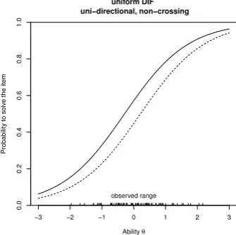
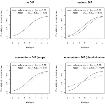
3.2.2 Uniform and non-uniform differential item functioning . . . 34
3.3 Methods to detect DIF or DIF groups . . . 38
3.3.1 Global model tests . . . 38
3.3.2 Methods to detect item-wise uniform DIF . . . 39
3.3.3 Methods to detect non-uniform DIF . . . 41
3.4 Rasch trees for uniform DIF detection . . . 42
4 Detecting non-uniform DIF with Rasch trees 49 4.1 Introduction . . . 49
4.2 Methods . . . 50
4.2.1 Logistic regression . . . 52
4.2.2 Rasch trees . . . 53
4.2.3 Extensions of the logistic regression . . . 57
4.3 Simulation study . . . 60
4.3.1 Manipulated variables . . . 61
4.3.2 Data generating processes . . . 62
4.3.3 Outcome variables . . . 64
4.4 Results . . . 65
4.4.1 No DIF . . . 65
4.4.2 Uniform DIF . . . 66
4.4.4 Non-uniform DIF: Discrimination condition . . . 70
4.4.5 On the classification accuracy . . . 70
4.4.6 On the detection of DIF groups . . . 75
4.5 Discussion . . . 76
5 A framework for anchor methods 79 5.1 Introduction . . . 79
5.2 The anchor process for the Rasch model . . . 80
5.2.1 Scale indeterminacy . . . 80
5.2.2 Item-wise Wald test . . . 81
5.2.3 Illustration of artificial DIF . . . 82
5.3 A conceptual framework for anchor methods . . . 84
5.3.1 Anchor classes . . . 84
5.3.2 Anchor selection strategies . . . 85
5.3.3 Anchor methods . . . 86
5.4 Appendix: Preliminary simulation study . . . 87
6 Anchor classes for DIF detection in the Rasch model 91 6.1 Introduction . . . 91
6.2 The iterative forward class and comparison methods . . . 92
6.2.1 The iterative forward anchor class and comparison anchor classes . . . 92
6.2.2 Anchor selection strategies . . . 93
6.2.3 Anchor methods . . . 93
6.3 Background of the simulation study . . . 96
6.4 Simulation study . . . 98
6.4.1 Data generating process . . . 98
6.4.2 Manipulated variables . . . 99
6.4.3 Outcome variables . . . 99
6.5 Results . . . 100
6.5.1 Null hypothesis: No DIF . . . 100
6.5.2 Balanced DIF: No advantage for one group . . . 102
6.5.3 Unbalanced DIF: Advantage for the focal group . . . 104
6.6 The impact of anchor contamination . . . 106
6.7 Characteristics of the anchor items inducing artificial DIF . . . 109
6.8 Summary and discussion . . . 112
6.9 Appendix . . . 116
7 Anchor selection strategies for DIF analysis in the Rasch model 123 7.1 Introduction . . . 123
7.2 Anchor methods . . . 125
7.2.1 The anchor process . . . 125
Contents iii
7.2.3 Anchor selection strategies . . . 128
7.3 Simulation study . . . 133
7.3.1 Data generating processes . . . 133
7.3.2 Manipulated variables . . . 134
7.3.3 Outcome variables . . . 135
7.4 Results . . . 135
7.4.1 Anchor selection for the constant four anchor class . . . 136
7.4.2 Anchor selection for the iterative forward anchor class . . . 138
7.4.3 Comparison of the mean test statistic and p-value threshold selection . 140 7.4.4 Comparison of the best performing methods . . . 141
7.4.5 Further simulated settings . . . 143
7.5 Discussion and practical recommendations . . . 145
8 Outlook on anchor selection strategies for multiple group comparisons 149 8.1 Introduction . . . 149
8.2 Alternative I: Selection of an anchor set for each paired comparison . . . 150
8.3 Alternative II: Selection of a common anchor set . . . 151
8.4 Discussion and future research questions . . . 153
9 Alternative ideas 155 9.1 Introduction . . . 155
9.2 Quasi-variances . . . 155
9.2.1 Basic idea of quasi-variances . . . 156
9.2.2 Quasi-variances in DIF detection . . . 156
9.2.3 Simulation study . . . 157
9.2.4 Results: Quasi-Wald tests versus Wald tests . . . 159
9.2.5 Results: Classification of the first anchor item . . . 161
9.3 Discussion . . . 163
9.4 Appendix . . . 164
10 Concluding remarks and outlook 169 10.1 Concluding summary and overview . . . 169
10.1.1 Selection of scientific findings . . . 170
10.1.2 Limits of this work . . . 171
1
1 Scope of this work
,,The importance of the property of invariance of item and
ability parameters cannot be overstated. This property
is the cornerstone of item response theory” according to
Hambletonet al.1991, p. 25.
The detection of differential item functioning (DIF) – i.e. the violation of the invariant item parameter assumption – is of utmost importance for the valid measurement of latent traits such as abilities in the field of educational testing, personality traits in behavioral research or attitudes in political and social sciences. If DIF is present, fair comparisons between groups of test-takers for example between participating countries in the PISA study and meaningful individual test results for example for test-takers in academic assessments are no longer guaranteed.
Recently, a new statistical method for the detection of uniform DIF in the Rasch model termed
Rasch treeswas suggested (Stroblet al., 2013). This approach brings together the model-based
recursive partitioning algorithm (Zeileiset al., 2008) and item response theory (IRT). This work addresses several challenges in the analysis of DIF, some of which are directly related to the newly proposed method and some that are concerned with the analysis of DIF in general.
This work is supported by the German Federal Ministry of Education and Research (BMBF) within the project “Heterogeneity in IRT-Models” (grant ID 01JG1060).
In Chapter 2, the model-based recursive partitioning algorithm (Zeileis et al., 2008) is intro-duced with regard to its potential for the social sciences. Methods developed from machine learning, such as classification and regression trees or random forests, are exploratory data min-ing techniques. They search for patterns over a set of available covariates and are popular in many fields such as epidemiology, genetics or economics due to their high performance (Strobl, 2008). However, research in the social sciences is based on the development and evaluation of theories to explain the object of research, such as human behavior, and might often not be-nefit from the exploratory nature of the algorithmic methods. Yet, the variant of model-based recursive partitioning can bring together a statistical modeling part and a variable selection part that indicates whether the parameters of the underlying model are unstable in groups defined by observable covariates. Thus, model-based recursive partitioning allows to evaluate whether statistical models, that represent the substantial theories, are appropriate for the entire sample. It can be used as a broad test of assumptions of pre-defined statistical models, for example to assess violations of Ockham’s razor.
It has already been shown to be a powerful tool for the detection of uniform DIF since it allows to detect observable groups that display different item parameters. The performance in word problems in a math test, for example, may depend on an additional trait dimension such as language skills and, thus, be harder for non-native speakers even if they have the same math ability. Rasch trees were developed as a global model test to answer the question if uniform DIF is present and – if so – which groups display DIF in the test. Chapter 3 briefly introduces the Rasch model, the problem of DIF, its relation to test fairness and several methods that were previously suggested for DIF detection with an emphasis on the Rasch trees.
In Chapter 4, it is evaluated whether Rasch trees are also suited for the detection of non-uniform DIF. Non-uniform DIF – as opposed to uniform DIF – is present when the disadvantages (mea-sured in terms of item parameter differences) vary over the ability range. In the math test example, it may happen that non-native speakers with a lower ability are more strongly affected by DIF compared to non-native speakers with a higher ability level. In this case, non-uniform DIF is present. For a comparison with the global Rasch tree procedure, two extensions of the logistic regression (that was suggested for the item-wise detection of uniform and non-uniform DIF by Swaminathan and Rogers, 1990) that allow to test for DIF in all items are suggested. It is shown that Rasch trees are also suitable for the detection of non-uniform DIF when large sample sizes are present and that they outperform the extensions of the logistic regression when DIF is simulated in the difficulty parameters or when the logistic regression is misspecified. Fur-thermore, Rasch trees automatically search for the affected groups over all available covariates and maintain their straightforward interpretation.
Up to Chapter 4 this work focused on global tests for DIF. While the global tests can be con-sidered as a first general assessment of measurement invariance, conclusions on the item level cannot yet be drawn. However, for practical research in test or questionnaire development, it is important to know which items display DIF and between which groups so that items can be modified or excluded from the test (Westers and Kelderman, 1992) and research on the under-lying causes of DIF (Jodoin and Gierl, 2001) can be carried out. Since DIF generally reflects situations where the latent ability is no longer unidimensional (Mellenbergh, 1982), the know-ledge about which items and groups display DIF may help to generate hypothesis about the additional dimensions involved.
To answer the question which items display DIF, item-wise DIF tests are regarded. Throughout this thesis, the classical Wald test based on the item parameters of the Rasch model (which are estimated using the conditional maximum likelihood) is used to assess DIF. For the DIF analysis, the origin of the scales of the item parameters has to be determined. Therefore, one linear restriction is imposed in each group and the items in the restriction are termed anchor
items or the anchor. There are two problems associated with the choice of the anchor that
is determined by an anchor method. First, the results of the DIF-analysis strongly depend on the choice of the anchor. Second, little information is at hand how the anchor is selected appropriately (Lopez Rivas et al., 2009). The Wald test is shown to be an appropriate test for DIF if it is combined with a suitable anchor method.
frame-1 Scope of this work 3
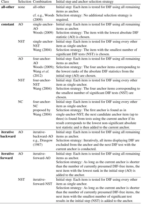
work for the classification of previously suggested anchor methods. In this framework, it is dis-tinguished betweenanchor classesthat determine characteristics of the anchor methods, such as a predefined number of anchor items, andanchor selection strategiesthat locate the anchor items. The entire procedure, consisting of an anchor class and – if necessary – an anchor selec-tion strategy, is then termedanchor method.
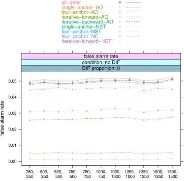
In this thesis, several new suggestions for the anchor process are proposed, since an appropriate anchor method is necessary for the correct classification of DIF- and DIF-free items. In case the anchor method does not work appropriately, inflated false alarm rates (i.e. DIF-free items erroneously display DIF) occur, that jeopardize the statistical inference at a predefined signif-icance level and, thereby, the correct classification of DIF- and DIF-free items. The inflated false alarm rate is induced by an artificial difference between the item parameters of the groups that also affects descriptive measures or effect size measures. In Chapter 6, a new anchor class named theiterative forward anchor classis developed for the DIF analysis of two pre-specified groups and evaluated in an extensive simulation study. While previously suggested methods often start with a criterion that is severely biased, this problem is avoided by starting with a single anchor item and successively including items in the anchor. The iterative forward anchor class generates a longer anchor and, thereby, allows for a higher hit rate (i.e. more DIF-items are correctly detected).
In Chapter 7, existing anchor selection strategies are compared with three new suggestions:
the mean p-value, the mean test statistic threshold and themean p-value threshold selection.
The anchor selections are combined with the newly proposed iterative forward anchor class and the previously suggested constant anchor class. In an extensive simulation study, it is shown that the anchor selection strategies developed in this thesis outperform previously suggested anchor selection strategies in the majority of the simulated settings and allow for a lower false alarm rate (i.e. less DIF-free items display DIF) and a higher hit rate (i.e. more DIF-items are detected).
So far, the development of the anchor class and anchor selection strategies was limited to the comparison of two groups. In Chapter 8, two alternative extensions of the anchor methods for multiple group comparisons are suggested. Even though several authors proposed to conduct post-hoc tests that answer the question which items display DIF between which groups (Kim
et al., 1995; Penfield, 2001), the literature on the anchor problem is – to my knowledge – limited
to the two-group case. The extension to multiple group comparisons is also important for the previously suggested Rasch trees that automatically detect – potentially more than two – groups of subjects that display DIF. To draw conclusions which items display DIF and between which groups, multiple comparison procedures need to be constructed (independently of whether they are used as post-hoc significance tests or as descriptive measures). Here, it is recommended to generalize the anchor methods for these comparisons by selecting a common set of anchor items. Therefore, two aggregation rules, themeanand theminimaxrule are suggested.
alternative to the decision that the first anchor item of a test was defined DIF-free is discussed and evaluated.
In Chapter 10, the contents of this thesis are briefly summarized. Furthermore, the main sci-entific findings are discussed followed by the limitations of this work. Finally, future research questions are addressed.
In summary, the suggestions presented in this thesis by means of new methods for DIF detection (Chapter 4), a new anchor class (Chapter 6) and new anchor selection strategies (Chapter 7) allow for lower false alarm rates (i.e. less items erroneously display significant DIF) and higher hit rates (i.e. true DIF-items are more often detected) compared to previous suggestions. In Chapter 8 extensions for multiple group comparisons were addressed to form the basis for post-hoc measures for the Rasch trees to answer the question which items display DIF between which groups.
1 Scope of this work 5
Contributing Manuscripts
Parts of this thesis are already published as a technical report, as a book chapter or a journal article. The rest are based on yet unpublished manuscripts. These manuscripts were developed in cooperation with coauthors. The titles of the manuscripts are listed below together with a short description of the content and the contributions from all authors.
• Kopf J., Augustin T. and Strobl C. (2013): The Potential of Model-based Recursive
Par-titioning in the Social Sciences – Revisiting Ockham’s Razor. In: McArdle J.J. and
Ritschard G. (Ed.): Contemporary Issues in Exploratory Data Mining, Routeledge, New York, to appear 2013.
In this manuscript, we review the model-based recursive partitioning technique and the predecessor method classification and regression trees. To highlight the potential of model-based recursive partitioning for the social sciences, we point out the relation of the algorithmic method to the principle of parsimony and Ockham’s Razor.
Julia Kopf identified the relation to Ockham’s Razor as one key argument for the use of model-based recursive partitioning in the social sciences, performed the analyses and drafted the manuscript. Carolin Strobl and Thomas Augustin contributed to the concep-tion and presentaconcep-tion of the article.
Chapter 2 is based on contents of this manuscript.
• Strobl C., Kopf J. and Zeileis A. (2013): Rasch Trees: A New Method for Detecting
Differential Item Functioning in the Rasch Model. Psychometrika, accepted.
This manuscript proposes a new method for DIF detection termedRasch treesbased on model-based recursive partitioning of the Rasch model. With this approach, it is possible to detect groups of subjects exhibiting DIF, which are not pre-specified, but result from combinations of observed covariates.
Carolin Strobl developed the idea to use the model-based recursive partitioning algo-rithm for DIF detection in the Rasch model, conducted the final simulation studies and drafted the manuscript. Achim Zeileis created the statistical software, contributed to the methodological aspects and to the manuscript. Julia Kopf reviewed the literature, derived measures necessary for the statistical test and conducted preliminary simulation studies during her master thesis.
Chapter 3, that forms the statistical background for the following methodological sugges-tions, is partly based on contents of this manuscript.
• Kopf J. and Strobl C. (2013): Detecting Non-uniform DIF with Rasch Trees.
proposed for the detection of uniform and non-uniform DIF, to allow for a direct com-parison.
Julia Kopf suggested the extensions of the logistic regression for the comparison, planned and performed the simulation studies and drafted the manuscript. Carolin Strobl identified the problem, developed the idea to detect non-uniform DIF with the Rasch trees and contributed to the presentation.
Chapter 4 is based on contents of this manuscript.
• Kopf J., Zeileis A. and Strobl C. (2013):Anchor Methods for DIF Detection: A
Compar-ison of the Iterative Forward, Backward, Constant and All-other Anchor Class. Technical
Report 141, Department of Statistics, LMU Munich.
This manuscript proposes a conceptual framework for categorizing anchor methods: The
anchor classto describe characteristics of the anchor methods and the anchor selection
strategyto guide how the anchor items are determined. Furthermore, we propose a new
anchor class termed the iterative forward anchor class and compare it to several previ-ously suggested anchor classes in an extensive simulation study.
Julia Kopf developed the conceptual framework, suggested the iterative forward anchor method, provided software for the anchor methods, conducted the simulation study and drafted the manuscript. Carolin Strobl contributed to the manuscript, especially regarding the interpretability of the results, and made methodological suggestions for consideration. Achim Zeileis provided one part of the software for the DIF tests and contributed to the formal notation in the manuscript.
Chapters 5 and 6 and are based on contents of this manuscript.
• Kopf J., Zeileis A. and Strobl C. (2013): Anchor Selection Strategies for DIF Analysis:
Review, Assessment, and New Approaches. Technical Report 150, Department of
Statis-tics, LMU Munich.
In this manuscript, we review existing anchor selection strategies that do not require any knowledge prior to DIF analysis – as this is typically not available in practical applica-tions – offer a formal notation for these strategies and propose three new anchor selection strategies. We evaluate the appropriateness of the anchor selection strategies by conduct-ing an extensive simulation study.
Julia Kopf developed the new threshold anchor selection strategies, implemented the an-chor selection strategies in statistical software, conducted the simulation study and drafted the manuscript. Carolin Strobl contributed to the presentation in the manuscript. Achim Zeileis provided parts of the software for the DIF tests, suggested the usage of p-values for anchor selection and contributed to the presentation of the manuscript.
Chapter 7 is based on contents of this manuscript.
• Kopf J., and Strobl C. (2013): Outlook on Anchor Selection Strategies for Multiple Group
1 Scope of this work 7
Ideas how anchor selection strategies can be generalized to paired multiple group compar-isons are presented in this manuscript draft. We argue to select a common set of anchor items instead of a different anchor set for each paired comparison. Two aggregation rules are introduced to generalize the anchor selection strategies for multiple group compar-isons.
Julia Kopf developed the generalization to multiple groups and drafted the manuscript. Carolin Strobl contributed to the manuscript.
Chapter 8 is based on contents of this manuscript draft and gives a first impression of current work in progress.
• Kopf J., and Strobl C. (2013):On Quasi-variances for DIF Detection.
Some alternative approaches to the strategies used in this thesis are presented in this manuscript draft. First, quasi-variances are evaluated regarding their appropriateness in DIF analysis. Second, the question whether the test decision for the first anchor item based on quasi-variances is better suited compared to the decision to declare the first anchor item as DIF-free is addressed.
Achim Zeileis developed the idea to use quasi-variances for DIF detection. Julia Kopf reviewed the methodological aspects, carried out the simulation study and drafted the manuscript. Carolin Strobl contributed to the manuscript.
9
2 The potential of model-based recursive partitioning in
the social sciences – Revisiting Ockham’s Razor
Summary: A variety of new statistical methods from the field of machine learning have the potential to offer new impulses for research in the social, educational and behavioral sci-ences. In this chapter we focus on one of these methods: model-based recursive partitioning. This algorithmic approach is reviewed and illustrated by means of instructive examples and an application to the Mincer equation, that is commonly used to describe the association be-tween education, job experience and income in econometric and sociological research. For readers unfamiliar with algorithmic methods, the explanation starts with the introduction of the predecessor method classification and regression trees. As opposed to classification and regression trees that search for groups of observations that differ in the values of a response variable, model-based recursive partitioning searches for groups differing in their estimated parameters of a postulated statistical model. With respect to the application and interpretation of model-based recursive partitioning, we highlight the principle of parsimony and Ockham’s Razor. To facilitate the applicability in the social sciences, we close with a section on recursive partitioning software available in the free R system for statistical computing.
Keywords: model-based recursive partitioning; structural change; parsimony; classification and regression trees (CART); algorithmic methods; data analysis
2.1 Introduction
The aim of this chapter is to demonstrate the potential of model-based recursive partitioning (Zeileiset al.2008; related approaches have previously been suggested by Loh 2002; Liet al.
2000; Chaudhuri et al. 1995, Wang and Witten 1997), a statistical method adopted from the field of machine learning, for applications in the social sciences. In particular, we will point out that this algorithmic method provides a powerful tool to evaluate whether relevant covariates have been omitted in a statistical model and, therefore, whether a theoretically postulated model is in conflict with Ockham’s Razor.
As a prototypical example the method is employed for evaluating the appropriateness of the so called Mincer equation (Mincer, 1974), which explains different income levels through rates of return from schooling and work experience by means of a linear model. The analysis relies on data of the German Socio-Economic Panel Study (SOEP) from 2008, provided by DIW Berlin (German Institute for Economic Research).
Hence, the objective of model-based recursive partitioning is related to the objective of latent class or mixture models where different regression parameter estimates are permitted between subgroups of the data set (see e.g. Vermunt, 2010; Leisch, 2004, for general introductions to mixture or latent class models, and ¨Unl¨u, 2011, for a specific application to knowledge struc-tures). In latent class regression models, these groups are unobserved, whereas in model-based recursive partitioning the groups are determined from combinations of observed covariates.
For example, in our investigation of the Mincer equation we will see that the intercept and the estimated coefficient for further education vary across groups of men and women working full-time in east or west Germany. Thus additional sociological and economic theories, such as discrimination in labor markets (e.g. Aigner and Cain, 1977; Phelps, 1972), need to be consid-ered for explaining these differences.
The method of model-based recursive partitioning forms an advancement of classification and regression trees, which are widely used in life sciences (cf. e.g. Hann¨overet al., 2002; Kitsantas
et al., 2007; Romualdiet al., 2003; Zhanget al., 2001) and have recently been applied to social
and behavioral sciences (e.g. Berk, 2006). Classification and regression trees will be summa-rized briefly in the following section, beginning with an informal description of the resulting tree-structure.
After some technical details of classification and regression trees are reviewed, the advanced method of model-based recursive partitioning is addressed in Section 2.3, firstly by pointing out the main differences and similarities to classification and regression trees. The review of model-based recursive partitioning will be continued by interpreting an instructive example and reca-pitulating the statistical background. To facilitate the use of this powerful algorithmic method in the social sciences, this chapter highlights the interpretation with regard to the principle of parsimony in the context of model construction (Section 2.4). Moreover, the application to the Mincer equation in Section 2.5 demonstrates the potential of model-based recursive partition-ing in empirical research. For further research, software available in the R system for statistical computing is indicated in Section 2.6.
In summary, in this chapter we show how model-based recursive partitioning allows to decide whether a postulated model fails to describe the whole sample in a suitable way, because the method may detect varying parameter estimates in different subgroups of the sample. Model-based recursive partitioning therefore offers a synthesis of the theory-based and the data-driven approach. In particular, it can be used for detecting violations of Ockham’s Razor. If sub-groups with different parameter estimates are found, the postulated model is too simple and not appropriate for the entire sample.
2.2 Classification and regression trees
2.2 Classification and regression trees 11
refers to regression trees. The basic principles of this approach will be explained by means of an exemplary application in the following section.
2.2.1 Basic principles of classification and regression trees
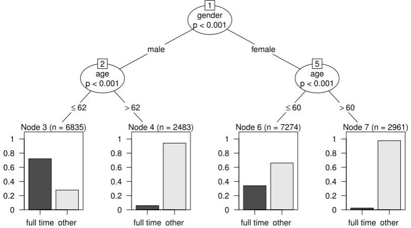
As a first example, we consider the respondents of the SOEP study 2008 (see Wagner et al., 2007, for details about SOEP). In this data set, groups of subjects vary with respect to whether they participate in full-time labor or not (the latter including all categories like part-time or marginally employment, civil or military service, vocational training and unemployment labeled here as ‘other’).
These groups can be described by means of covariates, such as age and gender. The covariates (here: age and gender), together with the response variable (full time or other), are handed over to the algorithm. The resulting tree-structure is displayed in Figure 1.
gender p < 0.001
1
male female
age p < 0.001
2
≤62 >62
Node 3 (n = 6835)
full time other 0
0.2 0.4 0.6 0.8 1
Node 4 (n = 2483)
full time other 0
0.2 0.4 0.6 0.8 1
age p < 0.001
5
≤60 >60
Node 6 (n = 7274)
full time other 0
0.2 0.4 0.6 0.8 1
Node 7 (n = 2961)
full time other 0
0.2 0.4 0.6 0.8 1
Figure 1– Classification tree: Assessing different frequencies of full-time jobs in
Germany (SOEP 2008). The resulting tree-structure shows varying
participation rates in full-time labor in three splits according to the covariates gender and age.
gender p < 0.001
1
male female
age p = 0.004
2
≤43 >43
Node 3 (n = 236)
0 500 1000 1500 2000 2500
Node 4 (n = 147)
0 500 1000 1500 2000 2500
marital p < 0.001
5
single{mar., mar.s, div., wid.}
Node 6 (n = 207)
0 500 1000 1500 2000 2500
Node 7 (n = 360)
0 500 1000 1500 2000 2500
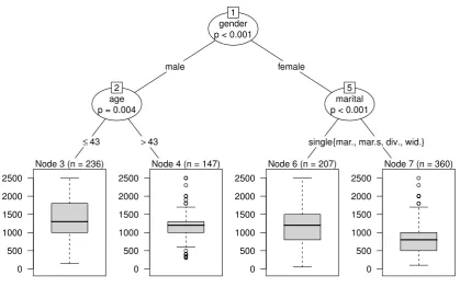
Figure 2– Regression tree: Assessing different requested incomes of unemployed
respondents (SOEP 2008). Three different levels are obtained in groups related
to gender, age and marital status.
The respective cutpoint for these splits depends on the type of the covariate: while gender has only two categories – male and female – and thus offers only one cutpoint, referring to age the algorithm must also find the ‘best’ cutpoint within this variable. This optimal cutpoint turns out to be located at the threshold of 62 years for the male subsample and 60 years for the female subsample (technical details are given below).
The resulting tree-structure is interpreted easily and shows groupwise frequencies for full-time and non-full-time workers in the end nodes: the left node indicates that the majority of men up to 62 years in Germany work full-time, while the majority of women up to 60 do not. Women over 60 years are hardly ever employed full-time. The tree-structure in this example represents an interaction effect between gender and age (see e.g. Strobl et al., 2009, for details on the interpretation of main effects and interactions in classification trees).
In contrast to this classification problem, regression trees focus on continuous response vari-ables. Instead of regarding the frequencies of the categories, groups with different average response values are separated and visualized, e.g. by means of box plots (like in Figure 2). These groups are again detected automatically.
2.2 Classification and regression trees 13
(nation) and marital status (marital). Figure 2 again shows the first split in the variable gender (node 1). The second split in the male subsample is again related to age (node 3 and node 4), while the third split in the female subsample is associated with marital status (node 6 and node 7). The cutpoint in a categorical variable is chosen automatically in an optimal way from all possible combinations of categories. Here the requested mean income is associated with marital status, in particular the request of female singles differs from the other categories (mar-ried, married but separated, divorced and widowed). The latter categories have smaller values of the requested income (median xmed = 800, mean x = 870) than female singles (xmed = 1200, x=1166), who seem to be in the same magnitude as men over 43 years (xmed = 1200,x=1159).
The highest average of requested income occurs within the male subsample up to the age of 43 years (node 3, xmed = 1300, x = 1349). After these three splits, all of the determined groups
are homogeneous enough to let the algorithm come to a stop, without further splitting, e.g. according to the nationality of the respondent. This exemplifies another attractive feature of partitioning methods: they implicitly perform a flexible variable selection.
A more detailed description of the technical procedure underlying classification and regression trees is given in the next section.
2.2.2 Some technical details
Classification trees search for different patterns in the response variable according to the avail-able covariates. Since the sample is divided in rectangular partitions defined by values of the covariates and since the same covariate can be selected for multiple splits, classification trees can assess even complex interactions, non-linear and non-monotone patterns. The structure of the underlying data-generating process is not specified in advance, but is determined in an entirely data-driven way. These are the key distinctions between classification and regression trees, and classical regression models. The approaches differ, firstly, with respect to the func-tional form of the relationship that is limited to e.g. linear influence of the covariates in most parametric regression models and, secondly, with respect to the pre-specification of the model equation in parametric models.
Historically, the foundations for classification and regression trees were first developed in the sixties as Automatic Interaction Detection (Morgan and Sonquist, 1963). Later the most pop-ular algorithms for classification and regression trees were developed by Quinlan (1993) and Breiman et al. (1984). Here we concentrate on a more recent framework by Hothorn et al.
(2006b), which is based on the theory of conditional inference developed by Strasser and We-ber (1999). The major advantage of this approach is that it avoids two fundamental problems of earlier algorithms for classification and regression trees: variable selection bias and overfitting (cf. e.g. Stroblet al., 2009).
discovered, the variable with the largest association is chosen for the split. Secondly, the best cutpoint in this variable is determined and used to split the sample into two groups according to values of the selected covariate. Then the algorithm recursively repeats the first two steps in the subsamples until there is no further violation of the null hypothesis, or a minimum number of observations per node is reached.
In the following, we briefly summarize which covariates can be analyzed using classification and regression trees, how variables are selected for splitting and how the cutpoint is chosen.
The response variable in the end nodes
As outlined in the previous section, classification trees search for groups of similar response values with respect to a categorical dependent variable, whereas regression trees focus on con-tinuous variables. Hothornet al. (2006b) stress that their conditional inference framework can be applied beyond that to situations of ordinal, censored survival times and multivariate re-sponse variables.
Within the resulting tree-structure, all respondents with the same covariate values – represented graphically in one end node – obtain the same prediction for the response, i.e. the same class membership for categorical responses or the same value for continuous response variables.
Selection of splitting variables
The next question is how the variables for the potential splits are chosen and how the related cutpoints can be obtained. As outlined above, Hothornet al.(2006b) provide a statistical frame-work for tests applicable to various data situations. In the binary recursive partitioning algo-rithm, each iteration is related to a current data set (beginning with the whole sample), where the variable with the highest association is selected by means of permutation tests as described in the following. The usage of permutation tests allows for evaluating the global null hypothesis
H0that none of the covariates has an influence on the dependent variable. IfH0 holds (in other words, if the independence between any of the covariates Zl (l = 1, . . . ,L) and the dependent
variable Y cannot be rejected), the algorithm stops. Therefore the statistical test acts both for variable selection and as a stopping criterion.
Otherwise the strength of the association between the covariates and the response variable is measured in terms of the p-value that corresponds to the test of the null hypothesis that the spe-cific covariate is not associated with the response. Thus, the variable with the smallest p-value is selected for the next split. The advantage of this approach is that the p-value criterion guar-antees an unbiased variable selection regardless of the scales of measurement of the covariates (cf. e.g. Hothornet al., 2006b; Stroblet al., 2007, 2009).
2.3 From classification and regression trees to model-based recursive partitioning 15
Selection of the cutpoints
After the variable for the split has been selected, we need a cutpoint within the range of the variable to find the subgroups that show the strongest difference in the response variable. In the procedure described here, the selection of the cutpoint is also based on the permutation test statistic: the idea is to compute the two-sample test statistic for all potential splits within the covariate. In the case of continuous variables all potential cutpoints between any two successive observations are investigated (except for a certain percentage of the smallest and largest obser-vations to avoid too small nodes). In the case of ordinal variables the ordering of the categories is accounted for. The resulting split is located where the binary separation of two data sets leads to the highest test statistic. This reflects the largest discrepancy in the response variable with respect to the two groups.
In the case of missing data, the algorithm proceeds as follows: observations that have missing values in the currently evaluated covariate are ignored in the split decision, whereas the same observations are included in all other steps of the algorithm. The class membership of these observations can be approximated by means of so called surrogate variables (Hothorn et al., 2006b; Hastieet al., 2008).
2.3 From classification and regression trees to model-based
recursive partitioning
Model-based recursive partitioning was developed as an advancement of classification and re-gression trees. Both methods originate from the field of machine learning, which is influenced by both statistics and computer sciences.
The algorithmic rationale behind classification and regression trees is described by Berk (2006, p. 263) in the following way:
”With algorithmic methods, there is no statistical model in the usual sense; no
ef-fort has been made to represent how the data were generated. And no apologies
are offered for the absence of a model. There is a practical data analysis
prob-lem to solve that is attacked directly with procedures designed specifically for that
purpose.”
In that sense, classification and regression trees are purely data-driven and exploratory – and thus mark the entire opposite of the theory-based approach of model specification that is preva-lent in the empirical social sciences.
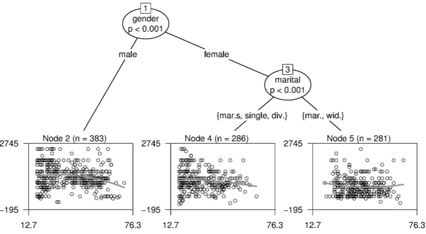
Figure 3– MOB: Assessing different relationships between age and requested income of unemployed respondents in Germany (SOEP 2008). The line pictures the estimated relationship in the current subsample and indicates the varying parameters according to groups related to age and marital status.
Technically, the tree-structure obtained from classification and regression trees remains the same for model-based recursive partitioning. However, instead of splitting for different pat-terns of the response variable, now we search for different patterns of the association between the response variable and other covariates, that has been pre-specified in the parametric model. Therefore the end nodes in the model-based tree represent statistical models, such as linear models, and no longer mere values of the response variable. The execution of a split in the model-based tree then indicates a parameter instability in the original model, i.e. the postulated model is too simple to explain the data.
2.3.1 Basic principles of model-based recursive partitioning
As an instructive example for a partitioned model, Figure 3 shows the tree-structure for a sample of unemployed respondents from the SOEP study. The model of interest here is the relationship between the requested income, at which respondents would take on a new job, and the age. The functional form of this relationship is fixed to a quadratic polynomial as often found intuitive for models relating age and income:
requested income=τ0+τ1·age+τ2·age2+ε.
Additional covariates passed over to the algorithm are marital status, gender and nationality.
2.3 From classification and regression trees to model-based recursive partitioning 17
with the linear and quadratic term is fitted, where the estimated coefficients ˆτ0,τˆ1, and ˆτ2 in-dicate parameter instability. The highest instability is related to gender and thus a split in this variable is performed. While in the sample of the male respondents (node 2) no more instabili-ties are detected, the female subset is again divided into two subgroups with differing parameter estimates. The end node in the middle shows the result for married but separated, single or divorced women (node 4). The rightmost end node contains the linear model for married and widowed women (node 5). Interestingly, even the direction of the relationship changes from a parabola on the left, where men of higher age tend to request less income, to a slight u-shape on the right, where married or widowed women request more income in higher age. The attractive feature of implicit variable selection is also maintained in model-based recursive partitioning: the nationality does not occur in any split decision in this example.
estimated coefficients
node number τˆ0 τˆ1 τˆ2
2 1014.5837 22.5446 -0.3618
4 1212.6621 -0.0236 -0.0871
5 1390.9708 -25.3983 0.2737
Table 1–Estimated coefficients of the regression models in the end nodes estimated from
the data sets that correspond to the end nodes.
In Table 1 the parameter estimates for the different groups – represented in the end nodes of the tree-structure – are displayed. The varying signs of the coefficients confirm what is illustrated in Figure 3: the inverse u-shape holds only for part of the sample and is reversed for other parts. Thus, the example illustrates that model-based recursive partitioning is indeed able to detect different functional forms which might be masked when a single model is fit to the data.
The example also shows that, as opposed to classification and regression trees, the end nodes in model-based recursive partitioning do not contain values of a response variable, but represent a statistical model for each specific subpopulation. Between these groups the estimated param-eters of the common underlying model vary significantly, but the postulated basic functional form (here polynomial) stated by the researcher is fixed. Within the subgroups no significant parameter instability is present.
Hence, the interpretation of a tree without any split is quite simple: there are no significant pa-rameter instabilities found in any of the covariates handed over to the algorithm. If, however, a tree-structure is displayed, it reveals that the postulated model is not appropriate for describing the entire sample. The variation of the parameters highlights structural differences in the ob-tained subgroups, which can be easily interpreted by examining the estimates or the graphical output.
2.3.2 Some technical details
The model-based recursive partitioning algorithm maintains the fundamental steps of the parti-tioning method reviewed in Section 2.2, but coherently extends them in the light of the model-based paradigm. According to this paradigm, the recursive process now estimates the basic sta-tistical model beginning with all available observations. The result of this step is the estimated parameter vector from the optimization of the objective function, typically the (log-)likelihood. In almost the same manner as classification trees, the recursive process starts: instead of test-ing the association, now the parameter instability is assessed ustest-ing so called generalized M-fluctuation tests (Zeileis, 2005; Zeileis and Hornik, 2007). If the data indicate parameter insta-bility, the split of the parent node in two daughter nodes is executed. Relying on the data points in the new subgroups only, the algorithm again searches for parameter instability until no fur-ther significant instability is found, or anofur-ther stopping criterion is fulfilled. The resulting tree structure can be visualized as illustrated in the examples presented below, so that the different groups can be compared. Note, however that statistical tests conducted after model selection – such as significance tests for group differences after recursive partitioning – may be affected by the effects described by Leeb and P¨otscher (2005) and Berk et al.(2010), and should thus be based on new data.
This brief overview about the similarities and differences in the algorithms leaves some ques-tions that have yet to be explained: Which models can be partitioned recursively? How can we assess parameter instability and where are the optimal cutpoints in the covariates in model-based recursive partitioning? These questions are addressed in the next subsections, which are structured in the same way as Section 2.2.2.
The statistical model in the end nodes
The foundation of a general statistical framework for model-based recursive partitioning by Zeileiset al.(2008) allows using a variety of underlying statistical models, such as linear and logistic regression models. The wide range of applications emerges from the inclusion of several widely used test statistics in a unified approach (Zeileis, 2005) called generalized M-fluctuation tests.
Technically, the generalized M-fluctuation test used for the split decisions relies on the ob-jective function Ψ(.) of the parameter estimation, like least-squares and maximum-likelihood-estimation:
ˆ
ϑ=arg max
ϑ
n
X
i=1
Ψ(yi, ϑ), (1)
where yi (i = 1, . . . ,n) symbolizes the vector of all values of the dependent and independent
variables in the postulated model for subjecti, andϑrepresents the (potentially vector-valued) parameter. For reasons of simplicity, here we use the full sample notation and do not distinguish whether the underlying observations are the entire sample or a specific subgroup arising from the recursive application of the procedure.
2.3 From classification and regression trees to model-based recursive partitioning 19
function
ψ(yi, ϑ)= ∂Ψ(yi, ϑ)
∂ϑ , (2)
as outlined below.
In addition to the model specification, the algorithm requires categorical or numeric covariates – denoted asZl (l=1, . . . ,L) – for potential splits in the model-based tree.
Selection of splitting variables
After the first step of the algorithm – fitting the underlying model for the whole sample and obtaining a preliminary estimate ˆϑ– a test of parameter instability is performed. It is based on the statistical framework developed by Zeileis and Hornik (2007) to detect structural changes by fluctuation tests. In econometrics, these tests for structural changes are widely used to detect e.g. a drop in the expected value of a time series for a stock exchange due to an economic crisis.
To detect a systematic change in the parameter over the range of a covariateZl, the observations
are ordered according to their values ofZl. Under the null hypothesis of parameter stability, no
systematic structural change is present. The null hypothesis is rejected if one or more param-eters of the postulated model change significantly over the ordering induced by the covariate
Zl.
The construction of general test statistics relies on the partial derivatives of the objective func-tion, e.g. of the log-likelihood. The contributions of each individual observationito the deriva-tive of the objecderiva-tive function (i.e., to the score function) evaluated at the current parameter estimate,ψyi,ϑˆ, are ordered with respect to the potential splitting variableZl. The individual
contributionsψyi,ϑˆare depicted as vertical dashed lines for an instructive example in Figure 4 (left).
Under the null hypothesis, the individual contributionsψyi,ϑˆshould fluctuate randomly around the mean zero, whereas in Figure 4 (left) a clear structural change can be detected. To grasp this structural change statistically, we turn from the individual contributions to their cumulative sums in Figure 4 (right). Zeileis and Hornik (2007) proved the convergence of the cumulative sum process (also termed decorrelated empirical fluctuation process)
Wl(t)= Jˆ−
1
2n−
1 2
bn·tc
X
i=1
ψ
yi,ϑˆ (3)
against a Brownian bridge. The first part of the formula, ˆJ−12, denotes an estimator of the
covarianceCovψ(Y,ϑˆ). The summation over all bn·tcrefers to the first n·t(witht ∈[0; 1]) observations according to the order with respect to covariate Zl (for example the first 50%,
age
requested income
20 30 40 50 60
400
800
1200
1600
2000
2400
age
requested income
20 30 40 50 60
−4000
−2000
0
2000
4000
Figure 4– Structural change in the mean over age (artificial data). The left plot displays
the mean income over all age groups (dotted line) and the individual deviations (dashed lines), the right the cumulated deviations over the variable age.
40. The strength of this peak is used as a statistical measure for the strength of the parameter instability.
The asymptotic properties of the cumulative sum process allow for the construction of test statistics that are used for detecting the structural change (see Chapter 3.4). The test statistic for numeric variables is directly build from the empirical fluctuation process Wl(t), while the
test statistic for categorical variables takes into account that the categories and the observations within the category are not ordered. The result of Zeileis et al. (2008) also permits the com-putation of p-values and thus the statistical decision whether the parameters differ significantly from parameter stability. If parameter instability is detected, the algorithm selects the variable with the smallest p-value. Splitting continues until there is no further instability in any current node.
Selection of the cutpoint
In case of a splitting decision the cutpoint can be sought by a criterion that also includes the maximization of the objective function in the two potential subsamples. In the case of or-dered or numeric covariates, these subsamples can easily be defined as L(ξ) = {i|zil ≤ ξ} and
R(ξ)={i|zil > ξ}for a candidate cutpointξand the componentzilofzl.
The optimal cutpointξ?is determined by maximizing
X
i∈L(ξ)
Ψ
yi,ϑˆ(L)+ X
i∈R(ξ)
Ψ
yi,ϑˆ(R) (4)
over all candidate cutpointsξ. ˆϑ(L)and ˆϑ(R)are the estimated parameters in the subsets. In case of unordered categorical covariates all potential binary partitions need to be evaluated and the partition with the highest criterion is chosen for the split (Zeileiset al., 2008).
parame-2.4 Potential in the social sciences 21
ter instability found or another stopping criterion is satisfied (such as a minimum sample size in the current node) the algorithm continues searching for instability and splitting the current (sub-)data set in daughter nodes.
2.4 Potential in the social sciences
The application of model-based recursive partitioning offers new impulses for research in the social, educational and behavioral sciences. For the interpretation of model-based recursive partitioning, we would like to point out the connection to the principle of parsimony: follow-ing the fundamental research paradigm that theories developed in the social sciences should yield falsifiable hypotheses, the latter are translated into statistical models. The aim of model construction is thus to simplify the complex reality.
The decision on the complexity of the formulated model can be guided by “a working rule known as Occam’s Razor whereby the simplest possible descriptions are to be used until they
are proved to be inadequate” (Richardson, 1958, p. 1247). This rule implies the objective of
parsimonious model formulation: a model should be no more complex than necessary, but it also needs to be complex enough to describe the empirical data.
In the regression context usually the usage of sparse and simple models with few variables explaining the response are propagated (e.g. Gujarati, 2003) – as long as no relevant explana-tory variables are omitted. The strength of model-based recursive partitioning in this context lies in the power to let the data decide this question. Indeed, it offers the possibility to detect whether the suggested model is inadequate because relevant covariates are missing and it ex-plicitly selects these relevant covariates. If the algorithm executes at least one split, we obtain the statistical decision that the parameters are instable and the data are too heterogeneous to be explained by the postulated model. In this case, the presumed functional form does not describe the entire sample in an appropriate way and thus subgroups have to be constructed.
Moreover, the tree-structured results provide information which subgroups differ in their associ-ation patterns. This informassoci-ation can either be integrated into a revision of the substantial theory and the formulation of a new parametric model, or it should be pointed out in the interpretation that the postulated model applies only to a limited scope of subjects.
2.5 Empirical example
To illustrate the potential of model-based recursive partitioning further, we turn to another ex-ample, based on an extension of the so called Mincer equation. In the seminal econometric work of Mincer (1974) the logarithmic income is described as a function of the variables years of schooling (time edu) and full-time experience (included in linear and squared terms, full ex, full ex2).
The Mincer equation owes its popularity to the straightforward interpretation of the coefficients as approximated rates of return from education (cf. Bj¨orklund and Kjellstr¨om, 2002, for a criti-cal discussion). We focus on the following extension of the Mincer equation that also includes a dummy variable for further education on the job (further edu):
ln (income)=τ0+τ1time edu+τ2full ex+τ3 full ex2+τ4 further edu+ε,
with ε ∼ N(0, σ2I). Here we restrict the observations from the SOEP study to over 6000 respondents in full-time employments who are not in vocational training and earn more than 500 Euros monthly.
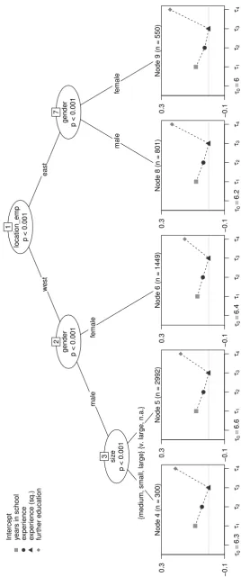
The examination of the Mincer equation, which is driven by the principle of parsimony, via model-based recursive partitioning is illustrated in Figure 5. The model formulation involves the effects (which are displayed as symbols in the end nodes) of years of schooling, further education and work experience in full-time jobs (linear and squared term) on the logarithmic gross income of fully employed respondents in Germany. Again, further potentially influencing variables are passed over to the algorithm, namely the location of the employer in east or west Germany, gender and the size of the company. The results show significantly different parameter estimates related to each of the additional covariates. These estimated coefficients of the Mincer equation are approximated rates of return e.g. from schooling. A closer look at the estimated parameters for the detected subgroups (Table 2) shows quite similar effects on the logarithmic income for some covariates from the original Mincer equation, such as the percentaged change for the time of education on earnings (ˆτ1). However, the estimated coefficients for further education (ˆτ4) and the intercept (ˆτ0) differ more strongly between the groups. In particular, the effect of further education (ˆτ4) is higher for employers in east as opposed to west Germany. Our results are in accordance with current empirical social and economic research on heteroge-neous effects of further education for men in Germany by Kuckulenz and Zwick (2005). One reason for the violation of a joint model for all respondents may lie in the strong assumption of the Mincer equation that there is no relevant change in the economy under research. In the SOEP study, this assumption is clearly violated by the reunification of the eastern and western parts of Germany. As a consequence, we find a split according to the location of the employer in east and west Germany in Figure 5.
2.5 Empirical example 23
location_emp p < 0.001
1
w
est
east
gender p < 0.001
2
male
female
siz
e
p < 0.001
3
{medium, small, large}
{v. large
, n.a.}
Node 4 (n = 300)
●
τ0
=
6.3
τ1 τ2 τ3 τ4
−0.1
0.3
Node 5 (n = 2992)
●
τ0
=
6.6
τ1 τ2 τ3 τ4
−0.1
0.3
Node 6 (n = 1449)
●
τ0
=
6.4
τ1 τ2 τ3 τ4
−0.1
0.3
gender p < 0.001
7
male
female
Node 8 (n = 801)
●
τ0
=
6.2
τ1 τ2 τ3 τ4
−0.1
0.3
Node 9 (n = 550)
●
τ0
=
6
τ1 τ2 τ3 τ4
−0.1
0.3
●
Intercept years in school exper
ience
e
xper
ience (sq.)
fur
ther education
Figure 5– Model-based recursive partitioning of the extended Mincer equation (SOEP
2008). The symbols in the end nodes illustrate the estimated coefficients in the
estimated coefficients
node number τˆ0 τˆ1 τˆ2 τˆ3 τˆ4
4 6.2743 0.0860 0.0430 -0.0009 0.2110
5 6.5620 0.0796 0.0335 -0.0005 0.1785
6 6.4486 0.0718 0.0369 -0.0007 0.1520
8 6.1543 0.0801 0.0340 -0.0006 0.2332
9 6.0173 0.0817 0.0258 -0.0004 0.2454
Table 2–Estimated coefficients of the regression models in the end nodes in Figure 5
estimated from the data sets that correspond to the end nodes.
explain the observed group differences.
2.6 Software
The data analysis presented here uses the R system for statistical computing (R Develop-ment Core Team, 2011), which is freely available under terms of the GNU General Public Li-cence (GPL) from the ComprehensiveRArchive Network athttp://CRAN.R-project.org/. Methods for classification, regression and model-based trees are provided in the packageparty.
• Conditional inference trees
The conditional inference framework is implemented in the functionctree()(Hothorn
et al., 2006b). It allows to compute both classification and regression trees.
• Model-based recursive partitioning
The model-based recursive partitioning algorithm is available via the function mob()
(Zeileis et al., 2008). At the moment the algorithm can be applied to various types of generalized linear models, survival models or linear models. Moreover, the authors al-low the users to build their own model classes and pass them on to the existing mob()
function. A vignette explaining the use of the software for linear regression and logistic regression trees including theR-code is also available (Zeileiset al., 2010).
Ongoing research expands the unbiased recursive partitioning approach presented here to psy-chometric models such as the Bradley-Terry model for detecting different preference structures (Stroblet al., 2011) as well as the Rasch model (Stroblet al.2010, Stroblet al.2013), that will be addressed in the next chapter, and factor analytic and structural equation models (Merkle and Zeileis, 2012) for the assessment of measurement invariance.
2.7 Concluding remarks
devel-2.7 Concluding remarks 25
opment of model-based recursive partitioning allows to combine the power of these algorithmic methods with that of theory-based parametric models by means of enhancing the purely data-driven approach towards a segmentation procedure for postulated models. Our presentation has highlighted the relation between this approach and the principle of parsimonious model construction. The tree-structured results allow straightforward interpretations of potential pa-rameter instabilities that have been detected via empirical fluctuation tests. The detection of parameter instability leads to the interpretation that the statistical model under investigation cannot describe the whole sample appropriately, because relevant covariates have been omitted. Thus, model-based recursive partitioning can be used as a diagnostic check for inadequately simple descriptions of the relationship between response and explanatory variables.
27
3 The issue of differential item functioning in the Rasch
model
Summary: The analysis of differential item functioning (DIF) in item response theory (IRT) research investigates the violation of the invariant measurement property among subgroups of examinees, such as male and female test-takers. Invariant item parameters are necessary to assess ability differences between groups in an objective, fair way. Questions addressed in this chapter are: What does DIF mean? What are potential consequences if DIF is present? How can DIF be detected?
The current state of research cannot be covered completely in the following sections. The in-troductory section raises historical and political aspects of DIF and is intended to motivate the analysis of DIF. Therefore, instructive examples as well as the main idea of commonly used statistical methods for DIF detection are included. The reader is referred to the monograph
Differential Item Functioning by Osterlind and Everson (2009), the like-titled collection by Holland and Wainer (1993) for more detailed information on DIF and to the broad collec-tion Rasch Models - Foundations, Recent Developments, and Applications by Fischer and Molenaar (1995).
Keywords: Differential Item Functioning, item bias, test fairness, statistical methods for DIF detection
3.1 The Rasch model
In the social and behavioral sciences, researchers are often confronted with the fact that the variable of interest is not directly observable. In sociology or in political science, attitudes towards certain political or social systems or subjects are not observable similar to personality traits in psychology or abilities and skills in educational research. Following the idea that the response behavior of test-takers contains information on thelatent variables, models from item response theory (IRT) are intended to measure variables that are not directly observable. The Rasch model (Rasch, 1960) is a widely used IRT model that displays unique statistical properties (Wang, 2004). When the assumptions of the Rasch model for measurement hold, measures of both, the item difficulty and the person ability, are generated on an interval scale level with a common measurement unit (Fischer, 1995). Furthermore, the assumptions of the model can be tested and, thus, the measurement process can be evaluated (Molenaar, 1995b).
In the Rasch model, the variableUi jcontains the dichotomous information whether the item or
the statement is solved or agreed to (Ui j =1) or not (Ui j =0) with the respective observed value
(ui j ∈ {0,1}). Here,θi denotes thelatent trait, e.g. the attitude, the ability or the personality trait
of person i (i = 1, ...,n) and βj denotes the difficulty of the item (also termed item location) or the extremeness of the statement j (j = 1, ...,k). For convenience, the latent trait will be called ability and the answer will be termed as solved an item (ui j = 1) or not (ui j = 0) in the
limited to variables measuring abilities or skills and it may provide useful insight to evaluate the appropriateness of the items or statements for measuring the latent trait in an objective, fair way.
In the Rasch model, the response of subjectito item jis modeled by
P(Ui j = ui j|θi, βj)=
eui j·(θi−βj)
1+eθi−βj (5)
and, thus, depends on two types of parameters, the item difficulty parametersβj and the person
ability parametersθi. The relationship between the latent trait and the probability of solving the item can be displayed in the so calleditem characteristic curves(ICCs) ortrace lines(Thissen
et al., 1988) oritem response functions(IRF) (Kimet al., 1994) as illustrated in Figure 6. Here,
four ICCs are displayed. In the Rasch model, the ICCs do not cross and all items are assumed to have to same discriminatory power. The item difficulty is defined as the value of the latent trait where the probability of solving the item equals.5.
−3 −2 −1 0 1 2 3
0.0
0.2
0.4
0.6
0.8
1.0
Item Characteristic Curve
Ability θ
Probability to solv
e the item
item 1 β1= −1 item 2 β2= −0.5 item 3 β3= +1.5 item 4 β4= +2
Figure 6– Different item characteristic curves that follow the Rasch model.
The ICCs in Figure 6 reflect the stringent assumptions of the Rasch model. Other IRT models for dichotomous responses such as the two-parameter logistic (2pl) model
P(Ui j =1|θi, αj, βj)=
eαj·(θi−βj)
1+eαj·(θi−βj) (6)