NUMERICAL ANALYSIS OF CO-CURRENT PARALLEL FLOW THREE FLUID HEAT EXCHANGER

784 | P a g e

NUMERICAL ANALYSIS OF CO-CURRENT

PARALLEL FLOW THREE FLUID HEAT

EXCHANGER

Akash Priy

1

, Sanjay Kumar Singh

2

1,2

Department of Mechanical Engineering, B.I.T. Sindri, (India)

ABSTRACT

This paper contains numerical analysis of a three fluid heat exchanger. The heat exchanger is of co-current parallel flow type .Results are obtained by varying the number of transfer units (NTU) and also varying the two dimensional longitudinal conduction parameter and the axial dispersion parameter. The performance analysis has been carried out numerically. Finite difference method has been used to discretize the non-dimensional form of energy equations and the iterations are obtained by Gauss-Siedel iterative technique. Results are obtained to optimize the losses due to the two dimensional longitudinal conduction and there is a major impact on the performance by varying the number of transfer units (NTU) of the three fluid heat exchanger.

Keywords-

Axial dispersion, Co-current, Heat exchanger, Longitudinal conduction, Three fluid.

I. INTRODUCTION

A heat exchanger is a device which is used to transfer the thermal energy i.e. heat between a solid object and a fluid or between two or more fluids. The fluid can be separated by a solid wall to prevent mixing (as in tube in tube type heat exchanger) or may be in direct physical contact as in cooling tower.Three fluid heat exchanger is a type of heat exchanger which involves the thermal interaction between three fluids. Three fluid heat exchanger are widely used in cryogenics technology and many other chemical processes such as purification and liquefication of hydrogen, ammonia gas synthesis, air purification and seperation systems, helium- air seperation system. In cryogenic technology we need to achieve a very very low temperature and this can be achieved by a compact multifluid heat exchanger by setting up of desired flow conditions and exchanging heat with the other streams. Apart from this the three fluid heat exchanger has its applications in aerospace industries where we need to achieve a certain fixed level of temperature.

785 | P a g e

classified as cocurrent, countercurrent and cocurrent- countercurrent type.Cross flow arrangements can also be further divided into single pass arrangements and multipass flow arrangements.

In past many researchers have tried to explain various aspects such as thermal performance, temperature distribution, effectiveness, size estimation of the three fluid heat exchanger. Morley [1] was the first to perform the analysis of three fluid heat exchanger. Based on the energy balances and rate equations, he got the temperature distributions of all the three fluid streams within the heat exchanger. Although he gave a formula but it was in dimensional form. Instead of giving the general solution he gave unknown coefficient of integration, which he decided to be evaluated in terms of boundary conditions. He neither presented the final explicit temperature nor does he define the design procedure. He gave a complicated heat exchanger sizing procedure which is a trial and error method and is very laborious too. Paschkis and Heisler [2] used an electric analogue method for the design of a parallel stream extended surface three fluid heat exchanger with three thermal communications. In this case he worked on the problems in which some of the inlet and outlet temperatures were specified and some parameters like length of heat exchanger and some unknown temperatures need to be found. The whole analysis was verified using a small heat exchanger model using fluids namely nitrogen, oxygen and air at low temperatures. Sorlie [3] developed a design theory He solved the three first order linear differential equations and derived some closed form formulas for the temperatures of the streams. He followed the effectiveness-NTU approach and

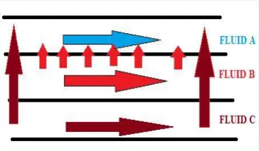
Figure 1(a) Co-current type three fluid heat exchanger with two thermal communication.

Figure 1(b) co-current type three fluid heat exchanger with three thermal communication.

787 | P a g e

A lot of paper has dealt with the temperature distribution of three fluid heat exchanger. This paper deals with the ways to optimize the three fluid heat exchanger for increased thermal performance and effectiveness. It also considers losses in the form of two dimensional longitudinal conduction and axial dispersion due to which the effectiveness of three fluid heat exchanger is largely reduced. We are also going to observe the effects on the performance of the three fluid heat exchanger by varying the number of transfer units (NTU) of the heat exchanger. In this paper numerical analysis of three fluid heat exchanger has been done with the help of a C program. Finite difference method has been adopted to discretize the non-dimensional form of energy equations and the iterations are obtained using Gauss Siedal iterative technique.

II. INDENTATIONS AND EQUATIONS

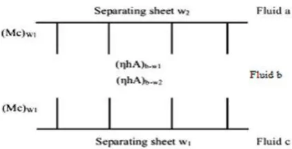
Figure 2 Distribution of convective resistance of central fluid ‘b’ and the

heat capacity of separating sheet with fins

A co-current type parallel flow three fluid heat exchanger with two thermal communication is one in which all the three fluid flows in the same direction and the third fluid exchanges the thermal energy with the other two. In Fig. 2, it is shown that the one fluid is flowing in between two separating sheets and having two thermal communications with the other two fluid. A similar type mathematical formulation has been given by Singh et al[15] in their technical note. Following are the assumptions made in this regard -

1. There is no phase change of any fluid in a three fluid system. 2. There is no source of heat generation within the fluids. 3. The fluid in centre is assumed to be hottest or the coldest. 4. No heat transfer to the surrounding.

5. The heat transfer area is uniformly distributed for each fluid. 6. Two thermal communication exists between the fluid.

7. Thermophysical properties of fluids streams and walls are assumed to be independent of space, time and temperature.

8. There is no variation in velocity and temperature of fluid streams in perpendicular direction of flow.

788 | P a g e

10.The fouling resistance and the film heat transfer coefficient are assumed to be constant and uniform.

11.Transverse conduction through fins between adjacent separating sheets is neglected. This implies there will be temperature extremum in the fin temperature profile.

12.Transverse thermal resistance of the separating sheets in a direction normal to it is considered negligible.

As the properties of the top and bottom fluid may be different in a general case therefore we need to consider two separating sheet walls in which the top separating sheet is depicted as (w1) whereas the bottom separating sheet wall is depicted as (w2).

The conservation of energy for the three fluid streams and for the two separating sheets can be expressed in non dimensional form for an infinitesimal small control volume.

For fluid streams a, b, c one gets Eqs. (5), (6), (7) respectively

1

Va Ta Eab Ta

Tw Ta

Rab  Rab X

       (1)









1 1 1 2 (1 ) Tb Tb

Vb Tw Tb Tw Tb

X

  

 

    

   (2)

2

Vc Tc Ecb Tc

Tw Tc

Rcb  Rcb X

 

  

  (3)

Similarly for separating sheets w1 and w2, the energy equations are given as Eqs. (4) and (5) respectively

1 1 1 1 1 2 1 ( ) ( ) 2 2 2 Tw Tw

Rab Ta Tw Tb Tw xNa

X Tw yNa Y  _{ }           _    (4)

2 _{2 1}

(1 ) ( 2) ( 2)

(1 )

2 2 ₂

2 2

Tw

Tb Tw Rcb Tc Tw

T Tw xNa yNa X Y        _  _          (5)

789 | P a g e

One need to replace the partial derivatives in the governing equations with discrete numbers. Discretization of partial differential equation is known as finite difference and discretization of the integral form of the equation is called finite volume. It is also needed a different type of coordinate system for transformation and grid generation. The term iscrete can be defined as unique , unconnected or a separate thing but the term discretization is a new and esoteric word. Analytic solutions of partial differential equations involves some closed form expression which give the variation of the dependent variables continuously throughout the domain. In constant numerical solutions can give answers at only discrete points in the domain, called Grid points. Uniform spacing greatly simplifies the programming of the solution , saves storage space and usually results is greater accuracy. The partial difference equations are totally replaced by the system of algebraic equation which can be solved for the values of the flow field variables at discrete points only. This method is Finite difference method.

The Gauss–Seidel method is an iterative technique for solving a square system of n linear equations with unknown x. Gauss siedel iterativetechnique is also known as method of successive displacement

III. METHOD OF SOLUTION-

The above equations from Eqs.1-5, are discretized with the help of finite difference method and the solutions are obtained by the Gauss – Siedal iterative techniques. The results are obtained in the tabular form by developing a C program. Graphs are drawn from the data obtained and the results are analysed to optimize the performance of the three fluid heat exchanger.

IV. RESULTS AND DISCUSSIONS

(a) Effects by varying the number of transfer unit(NTU) with no longitudinal conduction and axial dispersion are shown in Fig.3(a)-3(g).

790 | P a g e

Figure 3(c) Graph showing NTU=3 and no longitudinal conduction and axial dispersion

Fig.3 (d) Graph showing NTU=4 and no longitudinal conduction and axial dispersion

791 | P a g e

Fig.3 (e) Graph showing NTU=6 and no longitudinal conduction and axial dispersion

Fig.3 (g) Graph showing NTU=8 and no longitudinal conduction and axial dispersion

792 | P a g e

(b) Effects of two dimensional longitudinal conduction-

Fig.4 a Effect of varying longitudinal conduction parameter λ=0.025

Results are further obtained by varying the values of longitudinal conduction and keeping other parameters such as NTU, thermal heat capacity ratio and conductance ratio of the fluids as constant. Several graphs are plotted as shown in Fig.3(a) to Fig.3(d).

793 | P a g e

Fig.4 c Effect of varying longitudinal conduction parameter λ=0.075

Fig.4 d Effect of varying longitudinal conduction parameter λ=0.1

794 | P a g e

(c) Effects of axial dispersion-

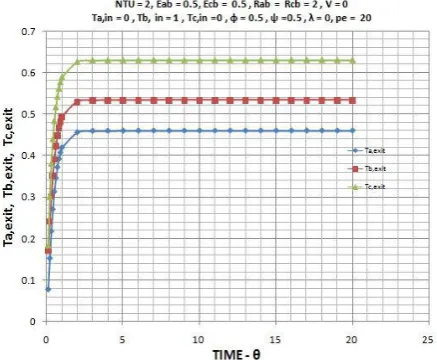
Figure 5 Graph for variation of axial dispersion parameter i.e. peclet number(Pe) = 20

We can observe that when we increase the peclect number let say from 5 to 20 or even more, the transient phase reduces and the graph reaches the steady state very quickly. Theoretically we can say that if the peclet number is infinite the performance of the three fluid heat exchanger is the highest. Butlosses due to eddies formation and surface irregularities deviates the flow condition and the axial dispersion is induced in the fluid. So we can see that the performance of three fluid heat exchanger decreases when we lower the peclet number from 20. The effect of axial dispersion dominates at lower values of peclet number.

.

V. CONCLUSION

Numerical analysis of co-current type parallel flow three fluid heat exchanger has been carried out. The above analysis was investigated numerically with the help of a computer program. It can be concluded that at lower values of NTU say 1-3 the performance is higher. And if we further increase the NTU from 4-8 the performance is decreased. At higher values of longitudinal conduction parameter the performance is lower.At lower values of Peclet number say upto 10 the performanceis lowered. Results obtained will surely help the design engineer in optimization of performance and design the three fluid heat exchanger.

VI. NOMENCLATURE

A area of heat transfer, C heat capacity rate (mc), W/K Ea,c-b capacity rate ratio = (mc)a,c/(mc)b h heat transfer coefficient, W/ K M mass flow rate of fluid, kg/s M mass of separating sheet, kg

795 | P a g e

NTU number of transfer unit

Pe Peclet number

Ra,c-b conductance ratio = (ηhA)a,c/(ηhA)b T dimensionless temperature =

(t−ta,in)/(tb,in−ta,in)

T dimensionless mean temperature U velocity of flow, m/s

V heat capacity ratio = LAcρc/Mcw X = (ηhA/mc)bx/Lx = Na(x/Lx) Y = (ηhA/mc)by/Ly = Na(y/Ly)

Greek letters

θ = (ηhA)bτ/(Mc)w, dimensionless time

φ = (ηhA)b−w1/(ηhA)b

η overall surface efficiency

λ longitudinal heat conduction parameter

ψ = (Mc)w1/(Mc)w

Subscripts

a,b,c fluid streams a,b and c

ex exit

in inlet

max maximum

min minimum

w separating wall

x,y x and y coordinate 1, 2 sheets 1 and 2

REFERENCES

[1] T. B. Morley Exchange of heat between three fluids, Engineer (1933) 155,134.

[2] V. Paschkis and M. P. Heisler() design of heat exchangers involving three fluids. Chem. Eng. Prog., Symp. Ser. 49, 65, (1953).

[3] T. Sorlie,Three-fluid heat exchanger design theory-counter and parallel flow, Technical Report 54 1962

Department of Mechanical Engineering, Stanford University, Stanford, California, (1962). [4] V.V.G , Krishnamurthy and Venkata Rao, Heat transfer in three fluid heat exchangers, Indian J.

Technol.2,(1964) 325-327.

796 | P a g e

[6] D. D. Aulds, R. F. Barron, Three-fluid heat exchanger effectiveness, Int. J. Heat MassTransf.10 (1967)

1457–1462.

[7] R. K. Shah, D. P. Sekulic, Thermal design theory of three-fluid heat exchangers, Adv. Heat Tran. 26 (1995) 219–328.

[8] D.P. Sekulic, A compact solution of the parallel flow three-fluid heat exchanger problem, Int. J. Heat Mass Transf. 37 (14) (1994) 2183–2187.

[9] Sarit Kumar Das, K. Murugesan, International Journal of Heat and Mass Transfer 43 (2000) 4327 - 4345 [10 ] S. Bielski, L. Malinowski, A semi-analytical method for determining unsteady temperature field in a

parallel-flow three-fluid heat exchanger, Int. Commun. Heat Mass Transfer 30 (8) (2003) 1071–1080. [11] M. Mishra, P.K. Das, S. Sarangi, Dynamic behaviour of three-fluid crossflow heat exchangers, J. Heat

Transf. 130 (1) (2008) (011801/1-6).