Simulated Annealing (SA) based Load Balancing Strategy for Cloud Computing

Simulated Annealing (SA) based Load Balancing

Strategy for Cloud Computing

Brototi Mondal#1, Avishek Choudhury#2 #1_{Department of Computer Science and Engineering,} Supreme Knowledge Foundation Group of Institutions,

Mankundu-712 139, India

#2_{Department of Computer Science, New Alipore College,} Kolkata-700053, India

Abstract

—

Keywords— Cloud computing; Load balancing;

Simulated Annealing;

I. INTRODUCTION

A model for convenient and on-demand network access to a shared pool of configurable computing resources that can be rapidly provisioned and released with minimal management efforts is cloud computing [1]. Its infrastructure is used by businesses and users to access application services from anywhere in the world on demand. Thus it represents as a new paradigm for the dynamic provisioning of computing services, typically supported by state-of-the-art Data Centers containing ensembles of networked Virtual Machines (VMs) [2]. The biggest and best known Cloud Computing providers include Amazon with EC2, Microsoft with Azure and Google with GoogleApps (e.g. Gmail, Google Docs, Google Calendar). Also, there are some popular large scaled applications like social-networking and ecommerce which are benefited by minimizing the costs using cloud computing. Due to the exponential growth of cloud computing it has been widely adopted by the industry and thus making a rapid expansion in availability of resources in the Internet. With the demand of large scale internet applications on cloud, both developers and researchers need to think about handling of massive requests. Whenever such an outburst occurs, the

primary challenge then becomes to keep the performance same or better. Thus in spite of glorious future of Cloud Computing, many critical problems still need to be explored for its perfect realization [3] and load balancing is one of these important issues.

To summarize, this paper makes the following contributions:  A soft computing approach based algorithm

Simulated Annealing (SA) has been used to solve this optimization problem to distribute the dynamic workload across multiple resources for achieving optimal resource utilization. More information on how this work differs from the other load balancing algorithms can be found in section II and section III.

 The performance of the proposed algorithm is compared with two commonly used scheduling algorithms FCFS and RR and a local search algorithm Stochastic Hill Climbing (SHC) [6] which is described in section IV.

The rest of this paper is organized as follows: Section II gives an overview of the related work; Section III discusses the basic features of Simulated Annealing (SA) algorithm along with the implementation details of our proposed SA based load balancing algorithm. The simulator environments as well as the simulation work loads are explained in Section IV. Also Section IV presents and analyses the experimental results and Section V concludes the study and highlights future work.

II. RELATEDWORK

Load balancing in the cloud differs from classical thinking on load-balancing architecture and implementation by using commodity servers to perform it. Load Balancing allows distribution of workload across one or more servers, data centers, hard drives, or other computing resources, thereby providing Cloud Service Providers (CSP) a mechanism to distribute application requests across any number of application deployments located in data centres [4].

is used to assign each job in arbitrary order to the nodes on which it is expected to be executed fastest, regardless of the current load on that node. Another approach [5] Min-Min scheduling algorithm calculates the minimum completion time for every unscheduled job and then the jobs are assigned with the minimum completion time to the node that offers it this time. Yang Xu et. al. has proposed a novel model to balance data distribution to improve cloud computing performance in data-intensive applications, such as distributed data mining [9]. A few soft computing techniques like Ant Colony [7] are also reported in literature. Some existing scheduling algorithms like Round Robin and FCFS for load balancing also exist. In our previous papers, we proposed a local search algorithm Stochastic Hill Climbing [6] and Genetic Algorithm [4] based load balancing approaches in cloud computing.

III.IMPLEMENTATIONDETAILS A. Load Balancing Using Simulated Annealing Load balancing is indispensable for cloud computing. Firstly, the cloud service provider (CSP) must use load balancing in its own cloud computing platform to provide a high efficient solution for the user. Secondly, a inter CSP load balancing mechanism is needed to construct a low cost and infinite resource pool for the consumer. Load balancing in cloud computing provides an organization with the ability to distribute application requests across any number of application deployments located in data centers and through cloud computing providers.

The procedures for solving an optimization problem are divided into two categories. Incomplete methods may not guarantee correct answers for all inputs. The well-known incomplete local search algorithm, Stochastic Hill Climbing that never makes "downhill" moves toward states with lower value, because it can get stuck on a local maximum. Complete methods which guarantee either to find a valid assignment of values to variables or prove that no such assignment exists. But they require exponential time in the worst case, which is not acceptable in the cloud computing domain. A purely random walk is complete but extremely inefficient. Simulated Annealing is an algorithm which combines hill climbing with random walk in some way that yields both efficiency and completeness.

B. Simulated Annealing

SA is a well known iterative improvement approach to optimization problems and also, it can be viewed as an algorithm used in statistical physics for computer simulation of the annealing of a solid to its ground state, i.e., the state with minimum energy. Given the set of configurations, a cost function and a neighbourhood structure, we can define the iterative improvement algorithm as follows. At the beginning of each iteration, a configuration i is given and a transition to a configuration j ϵ P(i) is generated where for each configuration i , P(i) is a subset of configurations, called the neighbourhood of i. If C(j) < C(i), the start configuration in the next iteration is j, otherwise it is i. If the transitions are generated in some exhaustive enumerative way, then the algorithm terminates by definition in a local minimum. Unfortunately, a local

minimum may differ considerably in cost from a global minimum. Simulated annealing can be viewed as an attempt to find near-optimal local minima by allowing the acceptance of cost-increasing transitions. More precisely, if i and j ϵ P(i) are the two configurations to choose from, then the algorithm continues with configuration j with a probability given by min{1 , exp(-(C(j) - C(i))/c)} where c is a positive control parameter, which is gradually decreased during the execution of the algorithm. Thus, c is the analogue of the temperature in the physical annealing process. Probability decreases for increasing values of C(j) - C(i) and for decreasing values of c, and cost-decreasing transitions are always accepted.

C. SA for Load Balancing in Cloud

The problem of load balancing can be formulated as allocating N number of jobs submitted by cloud users to M number of processing units in the Cloud at any particular instance of time .Each processing unit will have a processing unit vector (PV) which indicates the current status of processing unit utilization. PV consists of MIPS, indicating how many million instructions can be executed by that machine per second and β is the cost of execution of instruction and DL is delay cost. The delay cost is an estimate of penalty, which Cloud service provider needs to pay to customer in the event of job finishing actual time being more than the deadline advertised by the service provider ,

PV = g (MIPS, β, DL) (1)

Similarly each job submitted by cloud user can be represented by a job unit vector (JV). T represents the type of service required by the job, Software as a Service (SAAS), Infrastructure as a Service (IAAS) and Platform-as-a-Service (PAAS). NIC represents the number of instructions present in the job; this is count of instruction in the job determined by the processor. Job arrival time (AT) indicates wall clock time of arrival of job in the system and worst case completion time (wc) is the minimum time required to complete the job by a processing unit. Thus the attribute of different jobs can be represented by 2.

JV = g (T, NIC, AT, wc) (2)

The Cloud service provider needs to allocate these N jobs among M number of processors such that cost function C as indicated in equation 3 is minimized.

C = w1 * β (NIC ÷ MIPS ) + w2 *DL (3)

The acceptance probabilities Pij by

Pij(c) = min {1, exp ( - ( C(j) - C(i) ) / c ) } (5)

The proposed algorithm is given below:

Proposed Algorithm:

Step 1: Randomly initialize a set of processing unit and initialize the control parameter to a very large positive value.

Step 2: Repeat until the control parameter value reaches to the minimum:

Step 2 (a): Generate a random set of processing unit and calculate ΔE using equation 3.

Step 2(b): Select the new set of processing unit with probability Pij calculated using equation 5.

Step 2 (c): Repeat until inner loop break condition is met .

Step 2 (d): Decrease the temperature by a certain rate. Step 2(e): Goto step 2 loop.

Step 3: End

IV.EXPERIMENTALANALYSIS A. Simulation Environment

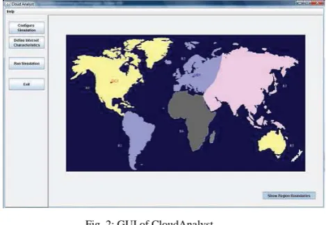
This research is conducted with CloudAnalyst [5] simulation toolkit which is modified with our proposed algorithm. One of the main objectives of CloudAnalyst is to separate the simulation experimentation exercise from a programming exercise, so a modeller can focus on the simulation complexities without spending too much time on the technicalities of programming using a simulation toolkit. The CloudAnalyst also enables a modeller to repeatedly execute simulations and to conduct a series of simulation experiments with slight parameters variations in a quick and easy manner. CloudAnalyst is capable of generating graphical output of the simulation results in the form of tables and charts, which is desirable to effectively summarize the large amount of statistics that is collected during the simulation. Its architecture in depicted figure 1 and a snapshot of the GUI of CloudAnalyst simulation toolkit is shown in figure 2.

CloudAnalyst provides modellers with a high degree of control over the experiment, by modelling entities and configuration options such as: Data Center, whose hardware configuration is defined in terms of physical machines composed of processors, storage devices, memory and internal bandwidth; Data Center virtual machine specification in terms of memory, storage and bandwidth quota.

B. SIMULATION SETUP

For simulating the proposed SA algorithm ,a hypothetical configuration has been generated keeping in mind the application of cloud in web-based e-mail system .As of January 2009 , over 500 millon people used Microsoft’s Web-based email, Hotmail or Windows Live Mail.

.TABLE I:CONFIGURATION OF SIMULATION ENVIRONMENT

S.No User

Base Region

Simultaneous Online Users During Peak

Hrs

Simultaneous Online Users During

Off-peak Hrs 1. UB1 0-N.America 5,70,000 57,000 2. UB2 1-S.America 7,00,000 70,000 3. UB3 2-Europe 4,50,000 45,000

4. UB4 3-Asia 9,00,000 90,000

5. UB5 4-Africa 1,25,000 12500 6. UB6 5-Oceania 1,50,000 30,500

Table I describes the simulation environment. The world is divided into six regions representing six major continents of the world.

Six “User bases” modeling a group of users representing the six major continents of the world is considered .It is assumed out of the total registered users 5% are online simultaneously during the peak time and only one tenth is on line during the off-peak.Size of virtual machines used to host applications in the experiment is 100MB. Virtual machines have 1GB of RAM memory and have 10MB of available bandwidth. Simulated hosts have x86 architecture.

Each simulated data centre hosts a particular amount of virtual machines (VMs) dedicated for the application. Machines have 4 GB of RAM and 100GB of storage. Each machine has 4 CPUs, and each CPU has a capacity power of 10000 MIPS. A time-shared policy is used to schedule resources to VMs.

Fig. 2: GUI of CloudAnalyst

C. RESULTS

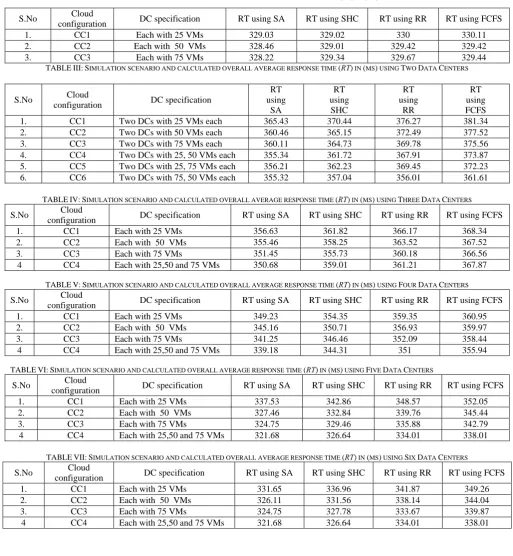
For experimentation several scenarios are considered. Experiment is started by taking one Data Center (DC) having 25, 50 and 75 VMs to process all the requests around the world.

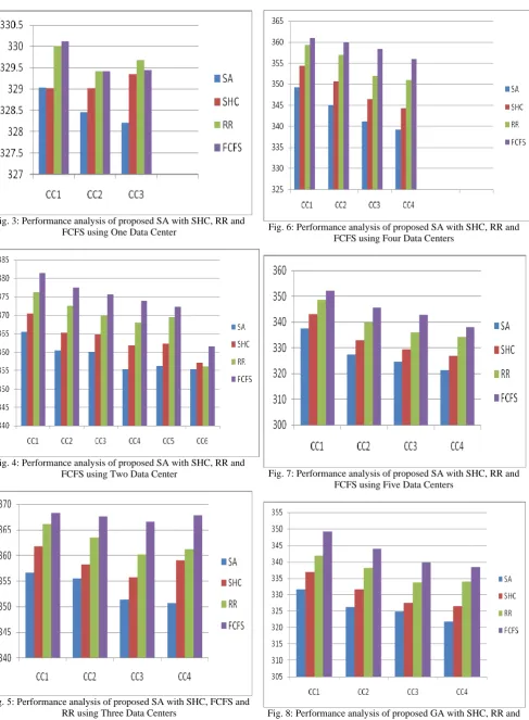
TABLE II describes this simulation setup with calculated overall average response time (RT) in ms for SA , SHC , RR and FCFS. The performance analysis graph for it is depicted in figure 3 where Cloud Configuration (CC) is

along x-axis and response time in ms is along y-axis. Next two DCs each having 25, 50, 75 VMs are considered as given in TABLE III and the corresponding graph is shown in figure 4. Subsequently three, four, five and six DCs are considered with combination 25, 50 and 75 VMs for each CCs as given in TABLES IV, V, VI and VII. The corresponding performance analysis graphs are displayed beside them in figures 5, 6, 7 and 8.

TABLE II: SIMULATION SCENARIO AND CALCULATED OVERALL AVERAGE RESPONSE TIME (RT) IN (MS) USING ONE DATA CENTER

TABLE III: SIMULATION SCENARIO AND CALCULATED OVERALL AVERAGE RESPONSE TIME (RT) IN (MS) USING TWO DATA CENTERS

TABLE IV: SIMULATION SCENARIO AND CALCULATED OVERALL AVERAGE RESPONSE TIME (RT) IN (MS) USING THREE DATA CENTERS

S.No Cloud

configuration DC specification RT using SA RT using SHC RT using RR RT using FCFS

1. CC1 Each with 25 VMs 356.63 361.82 366.17 368.34

2. CC2 Each with 50 VMs 355.46 358.25 363.52 367.52

3. CC3 Each with 75 VMs 351.45 355.73 360.18 366.56

4 CC4 Each with 25,50 and 75 VMs 350.68 359.01 361.21 367.87

TABLE V: SIMULATION SCENARIO AND CALCULATED OVERALL AVERAGE RESPONSE TIME (RT) IN (MS) USING FOUR DATA CENTERS

S.No Cloud

configuration DC specification RT using SA RT using SHC RT using RR RT using FCFS

1. CC1 Each with 25 VMs 349.23 354.35 359.35 360.95

2. CC2 Each with 50 VMs 345.16 350.71 356.93 359.97

3. CC3 Each with 75 VMs 341.25 346.46 352.09 358.44

4 CC4 Each with 25,50 and 75 VMs 339.18 344.31 351 355.94

TABLE VI: SIMULATION SCENARIO AND CALCULATED OVERALL AVERAGE RESPONSE TIME (RT) IN (MS) USING FIVE DATA CENTERS

S.No Cloud

configuration DC specification RT using SA RT using SHC RT using RR RT using FCFS

1. CC1 Each with 25 VMs 337.53 342.86 348.57 352.05

2. CC2 Each with 50 VMs 327.46 332.84 339.76 345.44

3. CC3 Each with 75 VMs 324.75 329.46 335.88 342.79

4 CC4 Each with 25,50 and 75 VMs 321.68 326.64 334.01 338.01

TABLE VII: SIMULATION SCENARIO AND CALCULATED OVERALL AVERAGE RESPONSE TIME (RT) IN (MS) USING SIX DATA CENTERS

S.No Cloud

configuration DC specification RT using SA RT using SHC RT using RR RT using FCFS

1. CC1 Each with 25 VMs 331.65 336.96 341.87 349.26

2. CC2 Each with 50 VMs 326.11 331.56 338.14 344.04

3. CC3 Each with 75 VMs 324.75 327.78 333.67 339.87

4 CC4 Each with 25,50 and 75 VMs 321.68 326.64 334.01 338.01 S.No Cloud

configuration DC specification RT using SA RT using SHC RT using RR RT using FCFS

1. CC1 Each with 25 VMs 329.03 329.02 330 330.11

2. CC2 Each with 50 VMs 328.46 329.01 329.42 329.42

3. CC3 Each with 75 VMs 328.22 329.34 329.67 329.44

S.No Cloud

configuration DC specification

RT using

SA

RT using

SHC

RT using

RR

RT using FCFS

1. CC1 Two DCs with 25 VMs each 365.43 370.44 376.27 381.34

2. CC2 Two DCs with 50 VMs each 360.46 365.15 372.49 377.52

3. CC3 Two DCs with 75 VMs each 360.11 364.73 369.78 375.56

Fig. 3: Performance analysis of proposed SA with SHC, RR and FCFS using One Data Center

Fig. 4: Performance analysis of proposed SA with SHC, RR and FCFS using Two Data Center

Fig. 5: Performance analysis of proposed SA with SHC, FCFS and RR using Three Data Centers

Fig. 6: Performance analysis of proposed SA with SHC, RR and FCFS using Four Data Centers

Fig. 7: Performance analysis of proposed SA with SHC, RR and FCFS using Five Data Centers

V. CONCLUSIONS

In this paper, we have proposed an efficient algorithm to distribute massive work load in cloud computing, based on a well-known optimization method, Simulated Annealing which can avoid becoming trapped at local minima. The performance analysis in terms of response time (ms) among the proposed SA algorithm and some existing algorithms shows that the proposed method not only outperforms but also guarantees the QoS requirement of customer requests. Though we have assumed that all the jobs are of the same priority which may not be the actual case, this can be accommodated in the JV and subsequently taken care in fitness function. Though SA algorithm based load balancing strategy balances the incoming requests among the available virtual machine efficiently, we shall strive to find more and more efficient methods using soft computing approaches for load balancing to obtain better results.

ACKNOWLEDGMENT

We would like to thank Prof. Kausik Dasgupta for his comments and reviews on this work. We also thank other reviewers for their feedback on the earlier draft of this paper.

REFERENCES

[1] “Security Issues and their Solution in Cloud Computing” ISSN (Online): 2229-6166, Prince Jain

[2] R. R.Buyya, R.Ranjan,” Intercloud: Utility-oriented federation of cloud computing environments for scaling of application services”,in: ICA3PP 2010, Part I, LNCS 6081., 2010, pp. 13–31.

[3] . Vouk, “Cloud computing- issues, research and implementations”, in Proc. of Information Technology Interfaces, pp. 31-40, 2008 [4] Kousik Dasguptaa, Brototi Mandalb, Paramartha Duttac, Jyotsna

Kumar Mondald, Santanu Dame, “A Genetic Algorithm (GA) based Load Balancing Strategy for Cloud Computing”:in CIMTA- 2013, Procedia Technology 10 ( 2013 ) 340 – 347

[5] B. Wickremasinghe, R. N. Calheiros and R. Buyya, “Cloudanalyst: A cloudsim-based visual modeller for analysing cloud computing environmentsand applications”, in Proc. of Proceedings of the 24th International Conference on Advanced Information Networking and Applications (AINA 2010), Perth, Australia, pp.446-452, 2010 [6] Brototi Mondal,Kousik Dasgupta and Paramartha Dutta, “Load

Balancing in Cloud Computing using Stochastic Hill Climbing-A Soft Computing Approach”, in Proc. of C3IT-2012, Elsevier, Procedia Technology 4(2012), pp.783-789, 2012.

[7] Ratan Mishra and Anant Jaiswal, “Ant colony Optimization: A Solution of Load balancing in Cloud”,in International Journal of Web & Semantic Technology (IJWesT), Vol.3, No.2, pp. 33–50, 2012 [8] T. R.Armstrong, D.Hensgen, The relative performance of various

mapping algorithms is independent of sizable variances in runtime predictions, in: 7th IEEE Heterogeneous Computing Workshop (HCW ’98), 1998, pp. 79–87