Consumption inequality and partial insurance

ISSN

1350-6722

University College London

DISCUSSION PAPERS IN ECONOMICS

CONSUMPTION INEQUALITY AND PARTIAL INSURANCE

by

Richard Blundell, Luigi Pistaferri and Ian Preston

Discussion Paper 03-06

DEPARTMENT OF ECONOMICS

UNIVERSITY COLLEGE LONDON

CONSUMPTION INEQUALITY AND PARTIAL INSURANCE

∗

Richard Blundell

University College London and Institute for Fiscal Studies.

Luigi Pistaferri

Hoover Institution, Stanford University and CEPR.

Ian Preston

University College London and Institute for Fiscal Studies.

September 2003

Abstract

This paper uses panel data on household consumption and income to evaluate the degree of

insurance to income shocks. Our aim is to describe the transmission of income inequality into

consumption inequality by contrasting shifts in the cross-sectional distribution of income growth

with shifts in the cross-sectional distribution of consumption growth. We combine panel data on

income from the PSID with consumption data from repeated CEX cross-sections. The results point

to some partial insurance but reject the complete market restrictions. We find a greater degree

of insurance for transitory shocks and differences in the degree of insurance over time and across

demographic groups. We also document the importance of durables and of taxes and transfers as

a means of insurance.

Key words: Consumption, Insurance, Inequality. JEL Classification: D52; D91; I30.

∗_{This paper is a revised version of “Partial Insurance, Information and Consumption Dynamics”. We thank Joe}

1

Introduction

Under complete markets agents can sign contingent contracts providing full insurance against

idiosyncratic shocks to income. Moral hazard and asymmetric information, however, make these

contracts hard to implement, and in fact they are rarely observed in reality. Even a cursory look

at consumption and income data reveals the weakness of the complete markets hypothesis. Thus

volatility of individual consumption is much higher than the volatility of aggregate consumption,

a fact against full insurance [Aiyagari, 1994]. Moreover, there is a substantial amount of mobility

in consumption [Jappelli and Pistaferri, 2003]. Indeed, Blundell and Preston [1998] use the growth

in consumption inequality over the 1980s in the U.K. to identify growth in permanent (uninsured)

income inequality. Formal tests of the complete markets hypothesis [see Attanasio and Davis,

1996], find that the null hypothesis of full consumption insurance is soundly rejected.1 Attempts

to salvage the theory by allowing for risk sharing within the family and no risk sharing among

unrelated families have also failed [Hayashi, Altonji and Kotlikoff, 1996].

In the textbook permanent income hypothesis the only mechanism available to agents to smooth

income shocks is personal savings. The main idea is that people attempt to keep the expected

marginal utility of consumption stable over time. Since insurance markets for income fluctuations

are assumed to be absent, the marginal utility of consumption is not stabilized across states. If

income is shifted by permanent and transitory shocks, self-insurance through borrowing and saving

may allow intertemporal consumption smoothing against the latter but not against the former.

This is simply because one cannot borrow to smooth out a permanent income decline without

violating the budget constraint, so that permanent shocks to income will be permanent shocks to

consumption.2 In this paper we start from the premise of some, but not necessarily full, insurance

and consider the importance of distinguishing between transitory and permanent shocks.

Models that feature a myriad of markets and those that allow for just personal savings as

a smoothing mechanism are clearly extreme characterization of individual behavior and of the

economic environment faced by the consumers. Deaton and Paxson [1994] notice this and envision

1

Notable exceptions are Altug and Miller [1990] and Mace [1991]. In these papers, however, failure to reject the null hypothesis of full consumption insurance is likely to be due to econometric and sample selection issues. See, e.g., Nelson [1994].

2

“the construction and testing of market models under partial insurance”, while Hayashi, Altonji

and Kotlikoff[1996] call for future research to be “directed to estimating the extent of consumption

insurance over and above self-insurance”. In this paper we address the issue of whether partial

consumption insurance is available to agents and estimate the degree of insurance over and above

self-insurance through savings. We do this by contrasting shifts in the distribution of income growth

with shifts in the distribution of consumption growth, and analyze the way these two measures of

household welfare correlate over time. Our research is related to other papers in the literature,

particularly Hall and Mishkin [1982], Altonji, Martins and Siow [2002], Deaton and Paxson [1994],

and Blundell and Preston [1998].

Using data from a combination of the Panel Study of Income Dynamics (PSID) and the

Con-sumer Expenditure Survey (CEX), we document a number of keyfindings. Wefind a strong growth

in permanent income shocks during the early 1980s. The variance of permanent shocks thereafter

levels off. The variance of consumption mimics these trends very closely. Wefind strong evidence

against full insurance for permanent income shocks but not for transitory income shocks, except for

a low income subsample where transitory shocks seem, unsurprisingly, less insurable. Further there

is evidence of some partial insurance of permanent income shocks (not uniform across demographic

groups); the results point to much of this partial insurance occurring through the adjustment of

durable expenditures. Finally we show that taxes and transfers provide an important insurance

mechanism for permanent income shocks.

We use the term partial insurance to denote smoothing devices other than credit markets

for borrowing and saving. There is scattered evidence on the role played by such devices on

household consumption. Theoretical and empirical research have analyzed the role of extended

family networks [Kotlikoff and Spivak, 1981; Attanasio and Rios-Rull, 2000], added worker effects

[Stephens, 2002], the timing of durable purchases [Browning and Crossley, 2001], progressive income

taxation [Mankiw and Kimball, 1992, Auerbach and Feenberg, 2001, and Kniesner and Ziliak, 2002],

personal bankruptcy laws [Fay, Hurst and White, 2002], insurance within thefirm [Guiso, Pistaferri

and Schivardi, 2003], financial markets [Davis and Willen, 2000], mortgage refinancing [Hurst and

Stafford, 2003], and the role of government public policy programs, such as unemployment insurance

stamps [Blundell and Pistaferri, 2003].

While we do not take a precise stand on the mechanisms (other than savings) that are available

to smooth idiosyncratic shocks to income, we emphasize that our evidence can be used to uncover

whether some of these mechanisms are actually at work, how important they are quantitatively,

and how they differ across households and over time. Our approach of examining the relationship

between consumption and income inequality follows the suggestion of Deaton [1995] that “although

it is possible to examine the mechanisms [providing partial insurance against income shocks], their

multiplicity makes it attractive to look directly at the magnitude that is supposed to be smoothed,

namely consumption”.

The distinction between permanent and transitory shocks stressed in this paper is an important

one, as we might expect to uncover less insurance for more persistent shocks. This point has

been emphasized in the early work on the permanent income hypothesis and also in the recent

analysis of limited commitment models. The literature on insurance under limited commitment

[Kocherlakota, 1996, Kehoe and Levine, 2001, Alvarez and Jermann, 2000] explores the nature

of income insurance schemes in economies where agents cannot be prevented from withdrawing

participation if the loss from the accumulated income gains they are asked to forgo becomes greater

than the gains from continuing participation. Such schemes, if feasible, allow individuals to keep

some of the positive shocks to their income and therefore offer only partial income insurance. The

proportion of income shocks which is insured will vary with the variance of the underlying shocks.

As the variance increases the value of future participation increases, alleviating the participation

constraint. Krueger and Perri [2001] investigate insurance of transitory shocks through analytic

solution of simple models and simulation of more complex cases and demonstrate the possibility

that consumption variance can actually fall with an increase in the variance of income shocks.

The results in Alvarez and Jermann demonstrate that if income shocks are persistent enough and

agents are infinitely lived, then participation constraints become so severe that no insurance scheme

is feasible. This suggests that the degree of insurance should be allowed to differ between transitory

and permanent shocks and should also be allowed to change over time and across different groups.

Uncovering the degree of partial insurance is likely to matter for a number of reasons. First,

on aggregation results [see Blundell and Stoker, 2002]. Second, it may help to understand the

characteristics of the economic environment faced by the agents. This may prove crucial when

evaluating the performance of macroeconomic models, especially those that explicitly account for

agents’ heterogeneity. Moreover, it is important to understand to what extent changes in social

insurance systems affect smoothing abilities, and the consequences of this for private saving

be-havior. This is important as far as the efficient design and evaluation of social insurance policy

is concerned. It is also particularly relevant in the US and the UK, where quantitatively large

changes in the structure of relative prices (most notably, wages) have occurred over the last three

decades. Much research exists about the rise in wage inequality, and we shall have very little to

add about this. Less evidence exists on consumption inequality [Cutler and Katz, 1992; Dynarski

and Gruber, 1997]. We show that consumption inequality follows closely the trends in permanent

earnings inequality documented, among others, by Moffitt and Gottschalk [1994].

A study of this kind requires in principle good quality longitudinal data on household

con-sumption and income. It is well known that the PSID contains longitudinal income data but the

information on consumption is scanty (limited to food and few more items). Our strategy is to

impute consumption to all PSID households combining PSID data with consumption data from

repeated CEX cross-sections. Previous studies [Skinner, 1987] impute non-durable consumption

data in the PSID using CEX regressions of non durable consumption on consumption items (food,

housing, utilities) and demographics available in both the PSID and the CEX. Although related,

our approach starts from a standard demand function for food at home (a consumption item

avail-able in both surveys); we make this depend on prices, total non duravail-able expenditure, and a host

of demographic and socio-economic characteristics of the household. Under monotonicity of food

demands these functions can be inverted to obtain a measure of non durable consumption in the

PSID. We review the conditions that make this procedure reliable and show that it is able to

reproduce remarkably well the trends in the consumption distribution.

The paper continues with an illustration of the model we estimate and of the identification

strategy we use (Section 2). In Section 3 we discuss data issues and the imputation procedure.

Section 4 contains a discussion of the results and a critical analysis of our finding. Section 5

Euler equation used in the empirical section and the imputation procedure.

2

Income and Consumption dynamics

2.1

The income process

The unit of analysis is a household, comprising a couple and, possibly, their children. Our

sample selection focuses on income risk and we do not model divorce, widowhood, and other

household breaking-up factors. We recognize that these may be important omissions that limit

the interpretation of our study. However, by focusing on stable households and the interaction

of consumption and income we are able to develop a complete identification strategy.3 We also

confine our analysis to links between labor income and consumption that become less important

after retirement. Consequently we only select households during the working life of the husband.

We assume that the main source of uncertainty faced by the consumer is income (defined as

the sum of labor income and transfers, such as welfare payments). We also assume that labor is

supplied inelastically and make the assumption of preference separability between consumption and

leisure. This means all insurance provided through, say, an added worker effect, will pass through

disposable income. Similarly, it is possible that the wage component of family income may have

already been smoothed out relative to productivity by implicit agreements within thefirm. If this

insurance is present, it will be reflected in the variability of income. The income process we consider

is:

yi,a,t=Zi,a,t0 ϕt+Pi,a,t+vi,a,t (1)

wherea and tindex age and time, respectively, y = logY is the log of real income, andZ is a set

of observable income characteristics. Note that we allow the effect of demographic characteristics

to shift with calendar time. Equation (1) decomposes unexplained income into a permanent

com-ponentPi,a,tand a transitory or mean-reverting component,vi,a,t. By writingyi,a,t rather thanyi,t

we emphasize the importance of cohort effects in the evolution of earnings over the life-cycle and,

more importantly, across generations entering the labor market in different time periods (and thus

3_{Whether stable families have access to more or less insurance than non-stable families is an issue that cannot}

facing different economic environments and opportunities). In keeping with this remark, we also

study consumption decisions of different cohorts.

For consistency with previous empirical studies [MaCurdy, 1982; Abowd and Card, 1989; Moffitt

and Gottschalk, 1994; Meghir and Pistaferri, 2003], we assume that the permanent componentPi,a,t

follows a martingale process of the form:

Pi,a,t=Pi,a−1,t−1+ζi,a,t (2)

where ζ_i,a,t is serially uncorrelated, and the transitory component vi,a,t follows an MA(q) process,

where the orderq is to be established empirically:

vi,a,t= q

X

j=0

θjεi,a−j,t−j

withθ0 ≡1. It follows that income growth is:

∆yi,a,t=∆Zit0ϕt+ζi,a,t+∆vi,a,t (3)

The covariance restrictions implied by (3) are explored in the next Section.

2.2

Self Insurance and Consumption Growth

Consider the optimization problem faced by householdi. Suppose the objective is to:

maxEa,t T_X−a

j=0

1 1 +Di,a+j,t+j

u(Ci,a+j,t+j) (4)

subject to the intertemporal budget constraints and the initial and terminal conditions onfinancial

assets:

Ai,a+j+1,t+j+1 = (1 +rt+j) (Ai,a+j,t+j +Yi,a+j,t+j−Ci,a+j,t+j) (5)

Ai,a,t given (6)

Ai,T,t+T−a = 0 (7)

where Di,a+j,t+j represents taste shifts, discount rate heterogeneity, etc. We set the end of the

life-cycle at ageT (and retirement at ageL), and assume that there is no interest rate uncertainty

credit markets are perfect, then one obtains the approximate Euler equation (see Appendix A.1 for

more details on the approximation):

∆ci,a,t∼=Γb,t+ξi,a,t+∆Zi,a,t0 ϑt+πi,a,tζi,a,t+γa,Lπi,a,tεi,a,t (8)

where ci,a,t = logCi,a,t is the log of real consumption, Γb,t a parameter that varies over time and

by cohort (indexed by b), ξ_i,a,t a random term, ∆Z_i,a,t0 are changes in observable characteristics

affecting tastes and impatience,γ_a,L is a weight that is an increasing function of age, andπi,a,t the

share of future labor income in the present value of lifetime wealth. In the empirical analysis we

assume that γ_a,L is a known constant rather than a parameter to estimate. The term Γb,t is the

slope of the consumption path for different year of birth cohorts, whileξ_i,a,t can be interpreted as

the individual deviation from the cohort-specific consumption gradient.4

For individuals a long time from the end of their life with the value of current financial assets

small relative to remaining future labor income,πi,a,t'1, and permanent shocks pass through more

or less completely into consumption whereas transitory shocks are (almost) completely insured

against through saving. Precautionary saving can provide effective insurance against permanent

shocks only if the stock of assets built up is large relative to future labor income, which is to sayπi,a,t

is appreciably smaller than unity, in which case there will be some smoothing of permanent shocks

through self insurance (see also Carroll, 2001, for numerical simulations). From here onwards,yand

c should be interpreted as the income and consumption components after removing demographic

characteristics and aggregate effects. The termsZi,a,t and Γb,t will thus be omitted from now on.

The remainder of this section considers the case πi,a,t '1 in which no part of permanent shocks

is insured through precautionary saving. We defer a discussion of the consequences of removing

this assumption to Section 4.4. To pre-empt, when we allow for partial insurance we are unable to

separately identify how precautionary saving (through πi,a,t) and partial insurance over and above

saving smooth the impact of shocks on consumption. However, this will be practically of little

importance. We will be identifying a parameter that combines self-insurance, partial insurance,

and perhaps even the crowding out effect of public insurance on private insurance. In other words,

we will still be able to pin down the degree of transmission of income shocks into consumption.

4

We assume that ζ_i,a,t,ξ_i,a,t and vi,a,t are mutually uncorrelated processes. The only source of

serial correlation, if present, arises from the transitory componentvi,a,t. Equation (3) can be used

to derive the following covariance restrictions in panel data

cov (∆ya,t,∆ya+s,t+s) =

½

var¡ζ_a,t¢+ var (∆va,t)

cov (∆va,t,∆va+s,t+s)

fors= 0

fors₆= 0 (9)

wherevar (.)andcov (., .)denote cross-sectional variances and covariances, respectively (the indexi

is consequently omitted). These moments can be computed for the whole sample or for individuals

belonging to a homogeneous group (i.e., born in the same year, with the same level of schooling,

etc.). The covariance term cov (∆va,t,∆va+s,t+s) depends on the serial correlation properties of v.

Ifv is anM A(q)serially correlated process, thencov (∆va,t,∆va+s,t+s)is zero whenever|s|> q+ 1.

Note also that ifvis serially uncorrelated (vi,a,t=εi,a,t), thenvar (∆va,t) = var (εa,t)+var (εa−1,t−1).

The moment restriction fors= 0in (9) can also be recovered from repeated cross-section data, an

observation underlying the analysis in Blundell and Preston [1998].

The panel data restrictions on consumption growth from (8) are as follows:

cov (∆ca,t,∆ca+s,t+s) = var

¡

ξ_a,t¢+ var¡ζ_a,t¢+γ2_a,Lvar (εa,t) (10)

for s = 0 and zero otherwise (due to the consumption martingale assumption). The equivalent

repeated cross-section moments are used in Blundell and Preston in conjunction with those relating

to income to separate the growth in the variance of transitory shocks to log income from the variance

of permanent shocks.

Finally, the covariance between income growth and consumption growth at various lags is:

cov (∆ca,t,∆ya+s,t+s) =

½

var¡ζ_a,t¢+γ_a,Lvar (εa,t) γ_a,Lcov (εa,t,∆va+s,t+s)

(11)

fors= 0, and s₆= 0respectively. Blundell and Preston note that the corresponding repeated cross

section moments give overidentification to their empirical analysis.

In the context of identifying sources of variation in household income and consumption, it

is worth stressing that the availability of panel data presents several advantages over a repeated

cross-sections analysis. In the latter case identification requires assuming that shocks are

cross-sectionally orthogonal to past consumption and income [see also Deaton and Paxson, 1994]. This

cov (∆ya,t,∆ca,t)with∆cov (ya,t, ca,t). This assumption will be violated if, say, knowledge of one’s

position in the income (or consumption) distribution conveys information about the distribution

of future shocks to income. In panel data, identification of the various parameters does not require

making such assumption and can allow for serial correlation in transitory shocks as well as

mea-surement error in consumption and income data. Finally, panel data provide more overidentifying

restrictions vis-à-vis repeated cross-section and thus can afford more flexibility in terms of model

testing.

As an example of the advantages offered by panel data, note for instance that identification of

the variances of shocks to income requires only panel data on income, not consumption. In the

simple case of serially uncorrelated transitory shock, for example:5

var¡ζ_a,t¢ = cov (∆ya,t,∆ya−1,t−1+∆ya,t+∆ya+1,t+1) (12)

var (εa,t) = −cov (∆ya,t,∆ya+1,t+1) (13)

We refer the reader to Section 4.2 for a discussion of the estimates of these variances.

2.3

Partial insurance

We now consider the possibility of partial insurance and suppose there are mechanisms (that we

do not model explicitly here but were discussed above) that allow insurance of a fraction¡1₋φ_b,t¢

and ¡1₋ψ_b,t¢ of permanent and transitory shocks, respectively. We might expectφ_b,t to be close

to unity andψ_b,tclose to zero. As noted above, precautionary saving might allow partial insurance

of permanent shocks if assets were large enough relative to future labor income (i.e. πi,a,t < 1),

but interpersonal insurance mechanisms might also underlie this.6 For simplicity of notation, we

confine ourselves to the case where the transitory shock is serially uncorrelated, consumption is

measured without error and var¡ξ_a,t¢= 0. These extensions are taken up in the empirical analysis.

In the partial insurance case residual income and consumption growth can be written,

respec-5_{See Meghir and Pistaferri [2003] for a generalization to serially correlated transitory shocks and measurement}

error in income.

tively, as:

∆yi,a,t = ζi,a,t+∆εi,a,t (14)

∆ci,a,t ∼= φb,tζi,a,t+ψb,tγa,Lεi,a,t (15)

The economic interpretation of the partial insurance parameter is such that it nests the two polar

cases of full insurance of income shocks (φ_b,t=ψ_b,t= 0), as contemplated by the complete markets

hypothesis, and no insurance (φ_b,t = ψ_b,t = 1), as predicted by the PIH with just self-insurance

through savings. A value0< φ_b,t<1(0< ψ_b,t<1) is consistent with partial insurance with respect

to permanent (transitory) shocks. The lower the coefficient, the higher the degree of insurance.

The relevant panel data moments are:

var (∆ya,t) = var

¡

ζ_a,t¢+ var (εa,t) + var (εa−1,t−1)

cov (∆ya,t,∆ya−1,t−1) = −var (εa−1,t−1)

cov (∆ya+1,t+1,∆ya,t) = −var (εa,t)

var (∆ca,t) = φ2b,tvar

¡

ζ_a,t¢+ψ2_b,tγ2_a,Lvar (εa,t)

cov (∆ca,t,∆ya,t) = φb,tvar

¡

ζ_a,t¢+ψ_b,tγ_a,Lvar (εa,t)

cov (∆ca,t,∆ya+1,t+1) = −ψb,tγa,Lvar (εa,t)

Sincevar (ζ)andvar (ε)can still be identified from panel data on income (thefirst three moments

above), there are only two parameters left to identify: φ_b,t and ψ_b,t. Take first the simple case

L₋a_{→ ∞} and r_→0 (γ_a,L→0). Then either:

φ_b,t= var (∆ca,t) cov (∆ca,t,∆ya,t)

(16)

or:

φ_b,t= cov (∆ca,t,∆ya,t)

cov (∆ya,t,∆ya−1,t−1+∆ya,t+∆ya+1,t+1)

. (17)

identify the extent of insurance against permanent shocks (ψ_b,t is obviously not identified). Under

these assumptionsφ_b,t would be overidentified and the overidentifying restrictions could be tested

using standard methods. Relaxing, as we do in our empirical work, the assumption that var¡ξ_a,t¢=

As a matter of interpretation, note that the numerator of (16) captures the variance of shifts

in consumption. In a model with no transitory shock effects on consumption, the volatility of

con-sumption growth depends only on the arrival of permanent shocks to income and the availability

of insurance mechanisms above self-insurance. The denominator of (16) measures the association

between consumption growth and income growth. In a model with no transitory shocks,

consump-tion growth tracks income growth only through its long run component. In the absence of partial

insurance mechanisms, the numerator and the denominator will be measuring exactly the same

(permanent) variability in income. Recall that in the self-insurance, infinite-horizon case any

per-manent shift in the variance of the distribution of income is paralleled by an equivalent perper-manent

shift in the variance of the distribution of consumption. With partial insurance, however, the

lat-ter is attenuated by the fact that permanent income shocks translate less than one-for-one into

consumption; the amount of attenuation (given by the ratio in (16)) is exactly measured by the

parameterφ_b,t.

In the more general case offinite horizon andr₆= 0, more complicated expressions are available

to identify the coefficients of interest. For instance,

ψ_b,t = γ−_a,L1 cov (∆ca,t,∆ya+1,t+1)

cov (∆ya+1,t+1,∆ya,t)

φ_b,t = cov (∆ca,t,∆ya,t+∆ya+1,t+1) cov (∆ya,t,∆ya−1,t−1+∆ya,t+∆ya+1,t+1)

and ψ_b,t and φ_b,t are generally overidentified even in this simple model.

Finally, it is very likely that measurement error will contaminate the observed income and

consumption data. Assume that both consumption and income are measured with multiplicative

(independent and quasi-classical) error,7 e.g.,

y_i,a,t∗ =yi,a,t+uyi,a,t (18)

and

c∗_i,a,t=ci,a,t+uci,a,t (19)

7

where x∗ denote a measured variable, x its true, unobservable value, and u the measurement

error. In Appendix A.2 we show that the partial insurance parameterφ_b,tremains identified under

measurement error.

2.4

Information

In the analysis presented so far we have assumed that in the innovation process for income

(14) the random variablesζ_i,a,t and εi,a,t represent the arrival of new information to the agentiof

ageain periodt. If part of this random term was known to the agent then the consumption model

would argue that it should already be incorporated into consumption plans and would not directly

effect consumption growth (15). Suppose a proportionκζ of the permanent shock was notknown

in advance to the consumer. Then the consumption growth relationship (15) would become

∆ci,a,t∼=φeb,tκζζi,a,t+ψb,tγa,Lεi,a,t. (20)

In this case the estimated φ_b,t would overstate the extent of partial insurance by the information

factor κζ.

The econometrician will treat ζ_i,a,t as the permanent shock. Whereas the individual may

have already adapted to this change. Consequently, although transmission of income inequality to

consumption inequality is correctly identified, the estimatedφ_b,thas to be interpreted as reflecting

a combination of insurance and information. This is discussed further in section 4.4 where we

interpret our empirical results.

3

The data

Our empirical analysis is conducted on two microeconomic data sources: the 1978-1992 PSID and

the 1980-1992 CEX. We describe their main features and our sample selection procedures in turn.

3.1

The PSID

Since the PSID has been widely used for microeconometric research, we shall only sketch the

description of its structure in this section.8

8

The PSID started in 1968 collecting information on a sample of roughly 5,000 households. Of

these, about 3,000 were representative of the US population as a whole (the core sample), and

about 2,000 were low-income families (the Census Bureau’s Survey of Economic Opportunities, or

SEO sample). Thereafter, both the original families and their split-offs (children of the original

family forming a family of their own) have been followed.

The PSID includes a variety of socio-economic characteristics of the household, including age,

education, labor supply, and income of household members. Questions referring to income are

retrospective; thus, those asked in 1993, say, refer to the 1992 calendar year. In contrast, many

researchers have argued that the timing of the survey questions on food expenditure is much less

clear [Hall and Mishkin, 1982; Altonji and Siow, 1987]. Typically, the PSID asks how much is

spent on food in an average week. Since interviews are usually conducted around March, it has

been argued that people report their food expenditure for an average week around that period,

rather than for the previous calendar year as is the case for family income. We assume that food

expenditure reported in survey year t refers to the previous calendar year, but check the effect of

alternative assumptions.

Households in the PSID report their taxable family income (which includes transfers and fi

-nancial income). The measure of income used in the baseline analysis below excludes income from

financial assets, subtracts taxes and deflates the corresponding value by the CPI. We obtain an

after-tax measure of income subtracting federal taxes paid. Before 1991, these are computed by

PSID researchers and added into the data set using information on filing status, adjusted gross

income, whether the respondent itemizes or takes the standard deduction, and other household

characteristics that make them qualify for extra deductions, exemptions, and tax credits. Federal

taxes are not computed in 1992 and 1993. We impute taxes for the last two years using regression

analysis for the years where taxes are available (results not reported but available on request).

Education level is computed using the PSID variable “grades of school finished”. Individuals

who changed their education level during the sample period are allocated to the highest grade

achieved. We consider two education groups: with and without college education (corresponding

to 13 grades or more and 12 grades or less, respectively).

PSID panel using data from 1978 to 1992 (the first two years are retained for initial conditions

purposes). Due to attrition, changes in family composition, and various other reasons, household

heads in the 1978-1992 PSID may be present from a minimum of one year to a maximum offifteen

years. We thus create unbalanced panel data sets of various length. The longest panel includes

individuals present from 1978 to 1992; the shortest, individuals present for two consecutive years

only (1978-79, 1979-80, up to 1991-92).

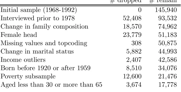
The objective of our sample selection is to focus on a sample of continuously married couples

headed by a male (with or without children). The step-by-step selection of our PSID sample is

illustrated in Table I. We eliminate households facing some dramatic family composition change

over the sample period. In particular, we keep only those with no change, and those experiencing

changes in members other than the head or the wife (children leaving parental home, say). We

next eliminate households headed by a female. We also eliminate households with missing report

on education and region,9 and those with topcoded income. We keep continuously married couples

and drop some income outliers.10 We then drop those born before 1920 or after 1959.

As noted above, the initial 1967 PSID contains two groups of households. The first is

repre-sentative of the US population (61 percent of the original sample); the second is a supplementary

low income subsample (also known as SEO subsample, representing 39 percent of the original 1967

sample). To account for the changing demographic structure of the US population, starting in 1990

a representative national sample of 2,000 Latino households has been added to the PSID database.

For the most part we exclude both Latino and SEO households and their split-offs. However, we

do consider the robustness of our results in the low income SEO subsample.

Finally, we drop those aged less than 30 or more than 65. This is to avoid problems related to

changes in family composition and education, in the first case, and retirement, in the second. The

final sample used in the minimum distance exercise below is composed of 17,788 observations and

1,788 households.

We use information on age and the survey year to allocate individuals in our sample to four

cohorts defined on the basis of the year of birth of the household head: born in the 1920s, 1930s,

9

When possible, we impute values for education and region of residence using adjacent records on these variables.

1 0_{An income outlier is defined as a household with an income growth above 500 percent, below}

1940s, and 1950s. Years where cell size is less than 100 are discarded.11

3.2

The CEX

The Consumer Expenditure Survey provides a continuous and comprehensive flow of data

on the buying habits of American consumers. The data are collected by the Bureau of Labor

Statistics and used primarily for revising the CPI. Consumer units are defined as members of a

household related by blood, marriage, adoption, or other legal arrangement, single person living

alone or sharing a household with others, or two or more persons living together who arefinancially

dependent. The definition of the head of the household in the CEX is the person or one of the

persons who owns or rents the unit; this definition is slightly different from the one adopted in the

PSID, where the head is always the husband in a couple. We make the two definitions compatible.

The CEX is based on two components, the Diary, or record keeping survey and the Interview

survey. The Diary sample interviews households for two consecutive weeks, and it is designed to

obtain detailed expenditures data on small and frequently purchased items, such as food, personal

care, and household supplies. The Interview sample follows survey households for a maximum of

5 quarters, although only inventory and basic sample data are collected in the first quarter. The

data base covers about 95% of all expenditure, with the exclusion of expenditures for housekeeping

supplies, personal care products, and non-prescription drugs. Following most previous research,

our analysis below uses only the Interview sample.12

The CEX collects information on a variety of socio-demographic variables, including

character-istics of members, charactercharacter-istics of housing unit, geographic information, inventory of household

appliances, work experience and earnings of members, unearned income, taxes, and other receipts

of consumer unit, credit balances, assets and liabilities, occupational expenses and cash

contribu-tions of consumer unit. Expenditure is reported in each quarter and refers to the previous quarter;

income is reported in the second andfifth interview (with some exceptions), and refers to the

pre-vious twelve months. For consistency with the timing of consumption, fifth-quarter income data

1 1

Median (average) cell sizes are 249 (219), 245 (246), 413 (407), and 398 (363), respectively for those born in the 1920s, 1930s, 1940s, and 1950s.

1 2_{There is some evidence that trends in consumption inequality measured in the two CEX surveys have diverged}

are used.

We select a CEX sample that can be made comparable, to the extent that this is possible,

to the PSID sample. Our initial 1980-1998 CEX sample includes 1,249,329 monthly observations,

corresponding to 141,289 households. We drop those with missing record on food and/or zero

total nondurable expenditure, and those who completed less than 12 month interviews. This is to

obtain a sample where a measure of annual consumption can be obtained. A problem is that many

households report their consumption for overlapping years, i.e. there are people interviewed partly

in yeartand partly in yeart+ 1. Pragmatically, we assume that if the household is interviewed for

at least 6 months att+ 1, then the reference year ist+ 1, and it istotherwise. Prices are adjusted

accordingly. We then sum food at home, food away from home and other nondurable expenditure

over the 12 interview months. This gives annual expenditures. For consistency with the timing of

the PSID data, we drop households interviewed after 1992. We also drop those with zero before-tax

income, those with missing region or education records, single households and those with changes

in family composition. Finally, we eliminate households where the head is born before 1920 or after

1959, those aged less than 30 or more than 65, those with outlying income (defined as a level of

income below the amount spent on food), and households entering the CEX after 1992. Our final

sample contains 15,380 households. Table II details the sample selection process in the CEX.

The definition of total non durable consumption is similar to Attanasio and Weber [1995]. It

includes food (at home and away from home), alcoholic beverages and tobacco, services, heating

fuel, transports (including gasoline), personal care, clothing and footwear, and rents. It excludes

expenditure on various durables, housing (furniture, appliances, etc.), health, and education. In

our empirical results we assess the sensitivity of our results to the inclusion of durables and other

non-durable items.

3.3

Comparing the two data sets

How similar are the two data sets in terms of average demographic and socio-economic

char-acteristics? Mean comparisons are reported in Table III for selected years: 1980, 1983, 1986, 1989,

and 1992.

difference in terms of family size and composition. The percentage of whites is slightly higher in

the PSID. The distribution of the sample by schooling levels is quite similar, while the PSID tends

to under-represent the proportion of people living in the West. Due to slight differences in the

definition of family income, PSID figures are higher than those in the CEX. It is possible that the

definition of family income in the PSID is more comprehensive than that in the CEX, so resulting

in the underestimation of income in the CEX that appears in the Table.

Trends in food expenditure are initially quite similar, but tend to diverge afterwards. One

explanation for this is that the wording of the food expenditure question in the CEX changed

several times over this period, resulting in PSID figures being higher than the corresponding CEX

figures. In particular, the CEX survey question asks about average monthly expenditure over

the last quarter in 1980-81, expenditure in an average week of the last quarter in 1982-87, and

reverts to the monthly expenditure question starting in 1988. Some researchers [Garner et al.,

1998] have noted that the change in the survey question induces a dramatic underestimation of

food expenditure in the CEX in the 1982-87 period. As we shall see, accounting for differences in

the way the food question is asked in the two data sets is crucial when replicating trends in average

consumption. Food away from home is, in contrast, under-reported in the PSIDvis-á-visthe CEX.

The last two rows of Table III compare the labor market activity of the household head and of

the spouse. Both male and female participation rates in the PSID are comparable to those in the

CEX.

3.4

The imputation procedure

In deriving the theoretical restrictions above, we have assumed that a researcher has access to panel

data on household income and total non-durable consumption. However, this is a very strong data

requirement. In the US, panel data typically lack household data on total non-durable consumption;

and those surveys, such as the CEX, that contains good quality data on consumption, lack a panel

feature. We may however combine the two data sets to impute non durable consumption to PSID

households. This of course requires making some assumptions detailed below.

The PSID collects data on few consumption items, mainly food at home and food away from

equation for food as a function of prices, demographics, labor supply variables, food away from

home and total non-durable expenditure. Within each cohort, variability of food consumption

is then explained by variability in those components plus unobserved heterogeneity, measurement

error, etc. We can invert this relationship to obtain a measure of the variability in total non-durable

consumption, one of the main objects of interest from the previous section. This inversion operation

requires consistent estimation of the parameters of the demand function for food and monotonicity

of the underlying demand function.

Our paper is not the first to combine CEX data with PSID data to impute a measure of

non durable consumption in the PSID [examples include Skinner, 1987; Bernheim, Skinner and

Weinberg, 2001; Dynan, 2000]. We adopt a demand function approach13 which we show is quite

successful in replicating the trends in the variance of consumption that are the main object of our

empirical analysis. To make matching of the two data sets feasible, the demand function for food

must be invertible with respect to total expenditure. This requires the demand function to be

monotonic in total expenditure.14 After some experimentation, we selected a loglinear functional

form. The main advantage of the loglinear demand function is that it provides “ready-to-use”

pre-dictions for total nondurable expenditure, avoiding, for instance, the problem of negative predicted

values faced when using the linear expenditure demand function. The loglinear demand function

has also a series of shortcomings, however. In particular, it cannot capture zero expenditures, it

does not satisfy adding up if applied to all goods in a demand system, and it does not capture

ap-parent non-linearities in Engel curve relationships. Nevertheless, these shortcomings do not appear

particularly relevant here. There are no zeros in food spending, the specification below is applied

to just one good, and the Engel curve for food is not far from being log linear.

Formally, we write the following demand equation for food at home in the CEX:

fi,a,t =Wi,a,t0 µ+β(Zi,a,t)ci,a,t+ei,a,t (21)

wheref is the log of food expenditure (which is available in both surveys), W contains prices, food

away from home and a set of demographics and labor supply variables (also available in both data

1 3

Skinner [1987] regresses non durable consumption on all the consumption items available in both surveys (food at home, food away from home, utilities, rents, etc.).

1 4_{While theoretically more appealing,flexible functional forms, such as variants of the AIDS model of Deaton and}

sets), c is the log of total non-durable expenditure (available only in the CEX), and e captures

unobserved heterogeneity in the demand for food and measurement error in food expenditure. We

allow for the elasticity β(.) to vary with time and with observable household characteristics.

We pool all the CEX data from 1980 to 1992. Our specification includes the log of the price

of food at home,15 the interaction of this with region of residence, the log of total nondurable

expenditure and its interaction with year dummies, education dummies and indicators for number

of children (no children, one child, two or three children, four children or more). We further

include indicators for male and female labor market participation and their interactions with the

number of children, food away from home,16 _{and a vector of demographics (an age spline, dummies}

for education and region of residence, year of birth dummies, indicators for number of children

as above, family size and its interaction with region dummies, and a dummy for whites). We

use the price of food at national level. Measurement error in nondurable expenditure biases the

expenditure elasticity towards zero; we thus instrument this variable with the log of before-tax

income (and interactions with demographics and year dummies).17 Standard errors are corrected

for time clustering. The estimation results are reported in Table IV.

We estimate an average expenditure elasticity of 0.66; this declines with education and increases

with the number of children. It also varies significantly with calendar time. The main effect is tightly

estimated, and so are most of the interactions.18 The estimate of the price elasticity is ₋0.9, and

is marginally significant. Interaction of the price variable with region dummies are insignificant.

Other demographics have the expected sign. Labor market participation reduces expenditure on

food at home (more strongly so for females); the effect of male participation is insignificant but

becomes stronger in the presence of more children.

Armed with the estimated demand parameters, we invert the demand equation for food and

ob-tain a measure of total nondurable expenditure in the PSID matching on observable characteristics

that are common to the two data sets. As explained in Appendix A.4, a good inversion procedure

should have two defining properties: (a) average (imputed) consumption in the PSID should

coin-1 5

We omit prices of other commodities due to multicollinearity problems.

1 6_{The inclusion of labor market participation variables and food away from home is justified by a conditional}

demand approach.

1 7_{This is important as far as replicating trends in consumption variance is concerned (see Appendix A.4).} 1 8

cide with average consumption in the CEX, and (b) the variance of (imputed) consumption in the

PSID should exceed the variance of consumption in the CEX by an additive factor (the variance of

the error term of the demand equation scaled by the square of the expenditure elasticity). If this

factor is constant over time the trends in the two variances should be identical.

As for the latter, trends in the variance of consumption are indeed remarkably similar in the two

data sets, as Figure 1 shows. Between 1980 and 1986 the variance of PSID imputed consumption

and the variance of CEX raw consumption are growing at a similar rate. Afterwards, they are

flat. The levels differ by a common factor as expected if the imputation procedure is reliable, see

Appendix A.4.

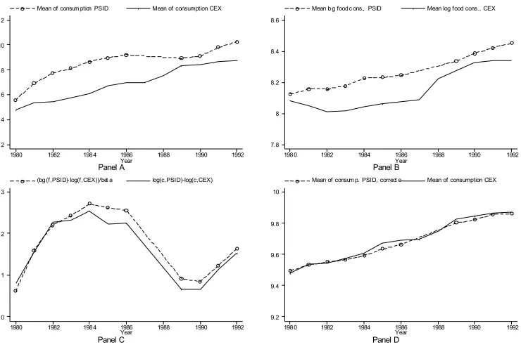
As for average consumption, our procedure appears to do less well. As shown in Panel A of

Figure 2, imputed average log consumption in the PSID tend to systematically exceed CEX average

log consumption. One reason for this divergence is, as noted above, that the food question is asked

differently in the two data sets, which may result in average food consumption (the main input

variable of our imputation procedure) being different as well. Panel B of Figure 2 shows that this

is indeed the case: in the 1982-1987 period CEX average food consumption (in nominal terms) is

dramatically different from PSID average food consumption. As shown in Appendix A.4, average

imputed consumption in the PSID may differ from average CEX consumption simply because

average food expenditure differs in the two data sets, not because the imputation procedure is

unreliable. Indeed, the overestimation of non-durable consumption in the PSID (Panel A) is the

mirror image of the underestimation of food expenditure in the CEX (Panel B). This is shown

in Panel C, where we plot the difference between PSID and CEX non-durable consumption and

between PSID and CEX food expenditure (scaled by the consumption elasticity). The two basically

coincide. Once we correct for this discrepancy, average consumption in the two data sets line up

remarkably well (see Panel D). Note that this is not “mechanically” true; using a biased estimate

of the consumption elasticity, for example, will not eliminate the discrepancy.

The evidence discussed in this section thus provides confidence in our use of imputed data

to estimate the parameters of interest discussed in Section 2. We now turn to the results of our

4

The results

We organize the empirical analysis in three parts: evidence on consumption inequality (section 4.1),

unrestricted consumption-income autocovariance estimation from the PSID (section 4.2), and

min-imum distance estimation using longitudinal data on household income and predicted consumption

(section 4.3). We then discuss ourfindings and a variety of experiments (Section 4.4).

4.1

Consumption Inequality and Income Uncertainty - Evidence from the CEX

Table V reports estimates of the variance of log consumption, the variance of log income, and their

covariance for all years and for four cohorts (born in the 1920s, 1930s, 1940s and 1950s).19 We

use data from 1980 to 1992 from the CEX. Figure 3 graphs income and consumption variances

and their covariance over the life cycle (we smooth trends using a rolling MA(3)). As said in

the previous Section, these trends are replicated by our imputed measure of consumption in the

PSID. For the two middle cohorts the variance of consumption increases throughout the sample

period (both variance grow very moderately in the second half of the 1980s). For the youngest

cohort the variance of income is flat while the variance of consumption actually declines. Finally,

for the oldest cohort both variances increase in the early 1980s and decline afterward. Trends in

covariances resemble those for the consumption variance (the level is higher). Two things are worth

noting: income inequality is higher and it grows more rapidly than consumption inequality. The

difference in the slopes of the two profiles is prima facie evidence against a simple model where

variances of shocks are stable and no insurance, apart from savings, is available. This simple model

would predict that income and consumption inequality grow at the same rate (the variance of

permanent shocks). Such a simple model is neither borne out visually by the data nor, as we shall

see, confirmed by more formal analysis below.

4.2

Autocovariance Estimates of Consumption and Income: Longitudinal

Evi-dence from the Matched PSID

The PSID data set contains longitudinal records on income and imputed consumption. We remove

the effect of deterministic effects on log income and (imputed) consumption by separate regressions

1 9_{These are the variances of deviations of consumption and income per household member from the cohort-specific}

of these variables on year and year of birth dummies, and on a set of observable family characteristics

(dummies for education, race, family size, number of children, region, employment status, residence

in a large city, outside dependent, and presence of income recipients other than husband and wife).

We allow for the effect of these characteristics to vary with calendar time. These variables reflect

deterministic growth in consumption and income (information). We then work with the residuals

of these regressions,ci,a,t and yi,a,t.

To pave the way to the formal analysis of Section 4.3, Table VI reports unrestricted minimum

distance estimates of several moments of interest for the whole sample: the variance of unexplained

income growth,var (∆ya,t), thefirst-order autocovariances (cov (∆ya+1,t+1,∆ya,t)), and the

second-order autocovariances (cov (∆ya+2,t+2,∆ya,t)). Estimates are reported for each year. Table VII

repeats the exercise for our measure of consumption. Finally, Table VIII reports minimum distance

estimates of contemporaneous and lagged consumption-income covariances.

Looking through Table VI, one can notice the strong increase in the variance of income growth,

especially in the early 1980s. Also notice the strong blip in the final year (in 1992 the PSID

converted the questionnaire to electronic form and imputations of income done by machine). The

absolute value of thefirst-order autocovariance also increases in the early 1980s and then is stable

or even declines after 1986. Second- and higher order autocovariances are small and only in few

cases statistically significant. At least at face value, this evidence seems to tally quite well with

a canonical MA(1) process, as implied by a traditional income process given by the sum of a

martingale permanent component and a serially uncorrelated transitory component:20

∆y∗_i,a,t=ζ_i,a,t+∆vi,a,t (22)

(with the permanent shockζ being serially uncorrelated and the transitory shockvpossibly MA(1),

i.e., vi,a,t = εi,a,t+θεi,a−1,t−1). Most attention has been paid to estimating the variance of the

two components ζ and v [Gottschalk and Moffitt, 1994; Blundell and Preston, 1998; Meghir and

Pistaferri, 2003]. In particular, their time trends can be used to understand whether the recent rise

in inequality has long- or short-run (instability) characteristics. This can be achieved by imposing

2 0_{Since evidence on second-order autocovariances is mixed, in estimation we allow for MA(1) serial correlation in}

the theoretical restrictions of equation (22) on the autocovariances of income at various lags as

reported in Table VI.

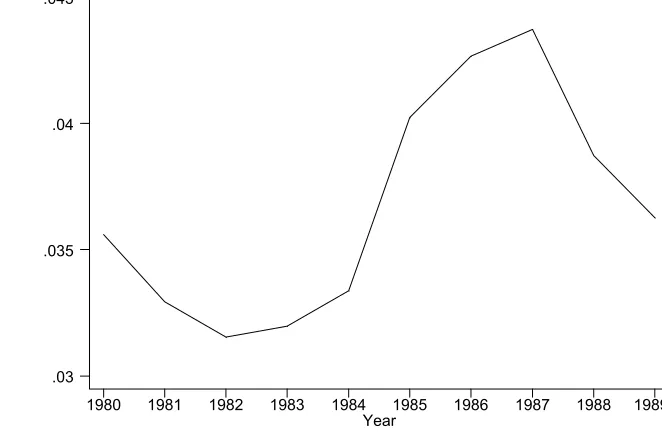
In Figures 4 and 5 we plot equally weighted minimum distance estimates of var¡ζ_a,t¢ and

var(εa,t), respectively, against time.21 Since estimates in the last two years are statistically

impre-cise, we focus only on the 1980s. Our results show a strong growth in permanent income shocks

during the early 1980s. The variance of permanent shocks levels offthereafter. The variance of the

transitory shock is basicallyflat in the period where the variance of permanent shock is increasing,

and it increases only when the variance of permanent shock slows down. This evidence is similar to

that reported by Moffitt and Gottschalk [1994] using PSID earnings data. It is also worth noting

that from trough to peak the variance of the permanent shock doubles, but the variance of the

transitory shock only goes up by about 50%.

While income moments are informative about shifts in the income distribution (and on the

temporary or persistent nature of such shifts), they cannot be used to make conclusive inference

about shifts in the consumption distribution. For this purpose, one needs to complement the

analy-sis of income moments with that of consumption moments and of the joint income-consumption

moments. This is done in Tables VII and VIII.

Table VII shows that the variance of imputed consumption growth increases quite strongly in

the early 1980s, peaks in 1984 and then it is essentially flat afterwards. Note the high value of

the variance which is clearly the result of our imputation procedure. The variance of consumption

growth captures in fact the genuine association with shocks to income, but also the contribution

of slope heterogeneity and measurement error.22 The absolute value of thefirst-order

autocovari-ance of consumption growth should be a good estimate of the variautocovari-ance of the imputation error.

This is in fact quite high and approximately stable over time. Second-order consumption growth

autocovariances are mostly statistically insignificant and economically small.

Table VIII looks at the association, at various lags, of unexplained income and consumption

growth. The contemporaneous covariance should be informative about the effect of income shocks

2 1

Since we cannot separately identify measurement error and transitory shock, the estimated variance of the transitory shock will also reflect the contribution of income data noise. In thefigures we smooth the estimates using simple 3-years moving averages.

2 2_{To afirst approximation, the variance of consumption growth that is not contaminated by error can be obtained}

on consumption growth if measurement errors in consumption are orthogonal to measurement errors

in income. This covariance increases in the early 1980s and then isflat or even declining afterwards.

The covariance between current consumption growth and future income growth cov(∆ya+1,t+1,∆ca,t)

should reflect the extent of insurance with respect to transitory shocks. Note that in the pure

self-insurance case and with infinite horizon, the impact of transitory shocks on consumption growth

is the annuity value ₁₊r_r . With a small interest rate, this will be indistinguishable from zero, at

least statistically. The addition of partial insurance ψ_b,t <1 makes this even more likely. In fact,

this covariance is hardly statistically significant and economically close to zero. As we shall see,

the formal analysis below will confirm this.

The covariance between current consumption growth and past income growth cov(∆ca+1,t+1,∆ya,t)

plays no role in the PIH model with perfect capital markets, but may be important in alternative

models where liquidity constraints are present. The estimates of this covariance in Table VIII are

close to zero. We should note, however, that for the low income sample examined further in the

empirical results below we dofind some sensitivity to transitory shocks. To sum up, there is weak

evidence that transitory shocks impact consumption growth or that liquidity constraints are

em-pirically important. In the sensitivity results reported below we note that there is more evidence of

responsiveness to transitory shocks for the low income poverty sample of the PSID. We now turn

to more formal minimum distance estimation, where we impose the theoretical restrictions outlined

in Section 2.3 on the unrestricted income and consumption moments of Table VI, VII, and VIII.

4.3

Partial Insurance

Here we focus on the results of a non-stationary model where the parameters vary across cohorts or

education groups (depending on the specification adopted) and time: in particular, we assume that

they shift at some point in the mid-1980s (consistent with most of the Figures or results discussed

above). We estimate the parameters that characterize the income and consumption process by

equally weighted minimum distance.23 Technical details are in Appendix A.3.

There are several parameters to estimate: the variances of the permanent and transitory income

2 3_{In general, the choice is between a non-linear least squares procedure (equally weighted minimum distance,}

shocks (σ2_ζ and σ2_ε, respectively), the MA coefficient θ of the transitory shock, the variance of

individual consumption gradients (σ2_ξ) and imputation error (σ2_u), the partial insurance coefficient

for the permanent shock (φ) and for the transitory shock (ψ). We assume L₋a _{→ ∞}and thus

the annuitization factorγ_a,L = r(1+r−θ)

(1+r)2 , whereθis the MA(1) parameter of the transitory income

component. We set r= 0.05.

Table IX reports the results of the model for the whole sample, two representative cohorts (born

in the 1940s and in the 1920s), and two education groups (with and without college education).24

Starting with income growth parameters, note that both the variance of the permanent shock

and the variance of the transitory shock are generally higher in 1985-92 than in 1979-84, which is

expected from the evidence given above. The MA parameter for the transitory shock is small and

generally not well measured. Turning to consumption parameters, note that the imputation error

absorbs a large amount of the cross-sectional variability in consumption in the PSID, anything

between 0.11 and 0.15. The variance of the imputation errorσ2_u is always precisely measured. The

variance of heterogeneity in the consumption slope is also sizable; it tends to be measured with

little precision when we stratify our sample by education or decade of birth.

In the whole sample the estimate of φ, the partial insurance coefficient for the permanent

shock, provides evidence in favor of partial insurance. In contrast, the evidence on ψ accords

with a simple PIH model with infinite horizon. In no case do we reject the null that there is full

smoothing with respect to transitory shocks (ψ= 0). The estimate ofφ should be compared with

the conventional belief, typical of simple consumption models, that permanent shocks to income

are permanent shocks to consumption. As said above, prudent individuals will attempt to smooth

this kind offluctuation by a greater extent than predicted by a model with quadratic preferences;

moreover, interpersonal insurance mechanisms or even public insurance will allow more smoothing

than predicted by simple models where markets for insuring shocks are all shut down. The scope

of the next subsections is to corroborate this evidence.25

Finally note that the insurance coefficient φ decreases between the early 1980s and the late

2 4

Results for other cohorts are available on request. We could not achieve convergence for the cohort born in the 1950s for the 1979-84 period due to the small number of observations.

2 5

1980s-early 1990s, suggesting that the degree of insurance has increased over this period. This may

also, however, reflect the nature of the permanent shocks that occurred over this period rather

than a change in the insurance mechanisms themselves.26 Moreover, the trend is not uniform

across groups: the less well educated and those born in the 1940s, for instance, face an increase in

φ. Finally, it is not clear that a formal test will reject the null of no change.

When the sample is stratified by year of birth or education, wefind qualitatively similar results:

there is evidence for partial insurance with respect to the permanent shocks, and full insurance

with respect to transitory shocks. The evidence across cohorts does not reveal any economically

interesting heterogeneity in the degree of insurance available to consumers, perhaps because of

small cell sizes that inflate standard errors; those with college education appear to be more able to

smooth consumption in the face of permanent shocks to income. For individuals without college

education and for the oldest cohort in our sample there is no statistically significant evidence for

insurance against permanent income shocks. For these groups, permanent shocks to income prompt

full consumption adjustment as in the traditional permanent income hypothesis model.

Finally, we note that the χ2 goodness of fit statistics reveal some support for our model

speci-fication despite its simplicity for certain of the periods and household types.

4.4

Discussion: Insurance and Measurement

In this section we provide further interpretation of our results and discuss potential sources of

bias in our estimates. Table X reports the results of various sensitivity checks where we change

our definition of consumption and income, and examine the effect of extending our sample to the

families of the SEO (the low-income subsample in the PSID), and of including young households

in our baseline sample. We use whole sample moments throughout.

4.4.1 Insuring Income Shocks through Durables

Consider that the PIH could hold with respect to total consumption rather than non-durable

con-sumption, the measure we use. The main consequence of this is that the Euler equation contains

2 6_{Suppose for example that permanent earnings shocks are the combination of permanent wage and employment}

an omitted variable, the growth in the fraction of total consumption that is devoted to non-durable

expenditure. In this caseφ_b,twill reflect, at least in part, the sensitivity of durable expenditure to

income shocks. It is possible to correct for this by extending our analysis to a measure of

consump-tion that includes durable expenditure. This is available in the CEX and our imputaconsump-tion procedure

can easily handle such extension.27 In columns (3) and (4) of Table X, we use a comprehensive

measure of consumption that includes durables and nondurables.28 This has a rather dramatic

effect on our results, as we nowfind no evidence for partial insurance with respect to permanent

shocks and again evidence for full insurance as far as transitory shocks are concerned. Indeed, we

cannot reject the restriction of φ equal unity and imposing this leaves the remaining results very

similar. This also suggests that it is unlikely that the information story of section 2.4 is

quantita-tively important, or else the estimate of φ would be less than one regardless of the consumption

measure used.

These results suggest that much of the insurance we estimate in the baseline model for

non-durables arises from optimal durable choice and timing, as argued, among others by Browning

and Crossley [2001]. One might expect the φcoefficient to rise simply because durables are more

income elastic than non durables. There are various other arguments in favor of including durables

in our measure of consumption and why that may also explain the lack of evidence for insurance.

In these arguments durable expenditure serves as an implicit insurance mechanism for non durable

consumption. The stock of durables can be upgraded or downgraded in response to permanent

shocks to income. Consider a permanent negative shock. In the absence of the durable hedge,

one should reduce non durable consumption by the same amount of the shock. Downgrading

one’s house, car etc., and slowing the rate of replacement can help smoothing the non durable

consumption effects of the permanent shock. A symmetric argument holds for a positive shock.

2 7_{See Meyer and Sullivan [2001] for a detailed discussion of the measurement of durables in the CEX.} 2 8

4.4.2 The Insurance Value of Taxes and Transfers

To see the impact of public insurance, suppose we exclude transfers (of any kind) from our measure

of income. If taxes and transfers provide insurance for permanent income shocks, the insurance

parameter in this specification should fall by an amount that reflects the degree of insurance. This

happens because consumption still incorporates any insurance value of taxes and transfers but the

new measure of income no longer does. The results of this experiment are reported in columns

(5) and (6) of Table X. A comparison with the baseline results shows that the estimated insurance

parameter declines from 0.6 to 0.52 in the early 1980s and from 0.48 to 0.26 in the second

sub-period. That is, by excluding transfers the partial insurance coefficient drops on average by 30%,

an estimate of the insurance provided by private and public transfers. This insurance can also be

seen through the change in the estimated variance of permanent and transitory shocks. With taxes

and transfers excluded, the variances of income shocks are indeed much higher.

4.4.3 Total Disposable Income

It has been suggested that people may use financial assets to hedge against labor market shocks,

including permanent ones [Davis and Willen, 2001]. Another experiment we consider is to include

income from assets in our definition of income. If portfolio choice is used to hedge against income

risk, addingfinancial income back in would induce an increase in the estimate ofφ, and such increase

would reflect the amount of insurance provided by portfolio choice. The results (reported in columns

(7) and (8)) are mixed, as in the original David and Willen’s paper. There is some evidence in

favor of this hypothesis, but the amount of insurance involved does not seem be quantitatively

important, probably due to lowfinancial market participation.

4.4.4 Precautionary Asset Accumulation

The assumption πi,a,t '1 made in Section 2.2 could be violated in the presence of precautionary

asset accumulation. This could be particularly relevant for cohorts close to retirement, and it would

signal partial insurance even when this is absent. However, focusing on young cohorts allows us to

address this point directly, because young individuals are a long time from retirement and have very