The number of initial states of the RC4 cipher with the same cycle
structure
Marina Pudovkina Moscow Engineering Physics Institute (State University)
Abstract. RC4 cipher is the most widely used stream cipher in software applications. It was
designed by R. Rivest in 1987. In this paper we find the number of keys of the RC4 cipher generating initial permutations with the same cycle structure. We obtain that the distribution of initial permutations is not uniform.
1. Introduction
RC4 cipher is the most widely used stream cipher in software applications. It was designed by R. Rivest in 1987. There are several papers by analysis of RC4, where several attacks and vulnerabilities were described. Most of these attacks revolve around the concept of a distinguisher. The first distinguisher was Golic [1] that exploited correlation between zi and zi+2. The results due
to [2, 3] and their generalization [8] are of most practical importance.
In [9] is introduced the idealized model of RC4 and considered the cipher as a random walk on a symmetric group. Mironov proved a necessary condition for existence of strong distinguishers in the idealized model.
In this paper we find the number of keys of the RC4 cipher generating initial permutations with the same cycle structure. We obtain that the distribution of initial permutations is not uniform. Thus, we show that the probability of generating the identical permutation is in π
4 / 1 2 / 3
2 / ) 1 (
+ −
+
m m
m
e m
more what you would expect.
2. Description of the RC4 cipher
The RC4 stream cipher is modeled by a finite automaton Ag= (F, f , Zm×Zm×Sm, Zm), where F: Zm×Zm×Sm→Zm×Zm×Sm is a next-state function, f: Zm×Zm×Sm→Zm is an output function. The
RC4 stream cipher depends on m=2n, n∈N .
The state of the RC4 cipher at time t is (it, jt, st)∈Zm×Zm×Sm and the initial state is (0, 0, s0,). Key schedule algorithm ρ
s0 is the identical permutation, i0=j0=0.
For t=1,m do: 1. it=t–1,
2. jt = jt-1 + st–1[it]+ kt-1(mod L) ( mod m),
3. st[it]= st–1[jt], st[jt]= st–1[it];
4. st[r]= st–1[r], r= 0,m−1\{it, jt}.
Consider the RC4 cipher at time t (t=1,2….).
1. it= it–1+1 (mod m );
2. jt = jt–1+ st–1[it] (mod m );
3. st[it]= st–1[jt], st[jt]= st–1[it];
4. st[r]= st–1[r], r= 0,m−1\{it, jt}. The output function f
Output: zt= st[( st[jt]+ st[it] )(mod m)].
Encryption xt: ct=xt⊕ zt. Decryption ct: xt=ct⊕ zt.
3. The number of states with the same cycle structure
In this section we prove our main result, i.e. we find the number of keys of RC4 generating initial permutations with the same cycle structure. We begin with definitions.
By B(α1,…,αm) denote the set of all permutations from Sm with the cycle structure
{1α12α2...mαm}, where 1⋅α
1+2⋅α2+…+m⋅αm=m. It is known that |B(α1,…,αm)|=
! !... ! ...
2 1
!
2 1 2
1
m m
m m
α α α
α α
α ⋅ ⋅ ⋅ . Let a permutation s∈Sm are chosen randomly from Sm, then P{s∈ B(α1,…, αm)}=
! !... ! ...
2 1
1
2 1 2
1
m m
mα α α α
α
α ⋅ ⋅ ⋅ .
Note that if the distribution of initial permutations ρ(k) of the RC4 cipher is uniform, then P{ρ(k)∈B(α1,…,αm)}=Ω(α1,…,αm) m
m
1 =
! !... ! ...
2 1
1
2 1 2
1
m m
mα α α α
α
α ⋅ ⋅ ⋅ , where Ω(α1,…,αm)=|{k∈
Zmm : ρ (k)∈ B(α1,…, αm)}|. The average of keys generating initial permutations with the same
cyclic structure is Nm(α1,…,αm)=
! !... ! ...
2 1 !
!
2 1 2
1
m m
m
m m
m m
α α α
α α
α ⋅ ⋅ ⋅
⋅ =
! !... ! ...
2
11 2 1 2
m m
m
m m
α α α
α α
α ⋅ ⋅ ⋅ .
Note that multiplication to the left transposition (it, jt) by st is swapped elements st[it] and
st[jt], i.e. st+1=(it, jt) st. Therefore, the initial permutation of RC4 can be represented as sm=(m–1, jm)…(1,j2) (0,j1)⋅E , where Е is the identical permutation.
Thus, we’ll consider the multiset ϑm={(m–1,jm)…(1,j2) (0,j1) | (jm,…, j1)∈Zmm }, which
elements are permutations that can be represented as (m–1,jm)…(1,j2) (0,j1), where k=1,m,
jk∈0,m−1. Note also that the permutation s can be represented as (m–1,jm)…(1,j2) (0,j1) different ways.
Let Aη={i1,…,iη}, | Aη|=η, be a directed set and i1< i2<…<iη. Let the set Jη={jη,…, j1},
where |Jη|≤η and either Jη∩ Aη=∅ or Jη∩ Aη≠∅. Denote ϖ=| Aη∪ Jη|.
Let us consider the product of transpositions (iη, jη)…(i2, j2) (i1, j1) that is generated by the
key-schedule algorithm of RC4.The product of transpositions (iη, jη)…(i2, j2) (i1, j1) corresponds to
the ϖ vertices graph Ξϖ that vertices are the elements of the set Aη∪Jη and that edges are the pairs
(ir, jr) labeled by ir, r=1 . Note that the transposition (,η α, α) is a loop of Ξϖ; the labels’ set of Ξη is
Aη and the number of edges is η.
The order relation on the set Aηis induced on the set of labels, i.e. i1< i2<…<iη on the labels’
set. For Aη={0,1,…,m–1}, Jη⊆Aη, η=m and ik=k–1, the product of transpositions (0,j1), (1,j2),…,(m–
1, jm) corresponding to some key of RC4 uniquely defines the graph Ξm.
We say that the connected graph Λn disintegrates into two cycles of length i and j, if the
product of transpositions corresponding to Λn can be represented as products of two independent
cycles of length i and j. By Γi,j denote a connected graph on i+j vertices labeled by elements of
X={x1, x2,…,xi+j} that disintegrates into two cycles of length i and j. To prove the main theorem we need the following proposition.
Proposition 1
1. The number Ni,j(n) of graphs Γi,j on i+j vertices, which are labeled by elements of the set {x1,x2,…,xi+j}, and having a length n cycle is
Ni,j(n)=
⋅ ⋅ − ⋅ ⋅ − − + + − − − + − − = − −
∑
1, 11 1
1
1
)
( j n k n k
n
k
k
i j A
i k n k k i n j i n j i
, (1)
2. The number Ni,j(n) of graphs Γi,j on i+j vertices, which are labeled by elements of the set {x1,x2,…,xi+j}
a) for i>0 and j>0 is
Ni,j=
∑
+= j i
n 2
⋅ ⋅ − ⋅ ⋅ − − + + − − − + − − = − −
∑
1, 11 1
1
1
)
( j n k n k
n
k
k
i j A
i k n k k i n j i n j i ,
b) for i>0, j=0 or j>0, i=0 is
Ni,0=jj–1,
where
∑
= + − + − = k t n t k
n k t
t n A
0
, ( 1) ,
1 ) 1
( k=0,n−1.
The proof is by direct calculations.
By Λ(ki,j) denote a graph with ki,j components that disintegrate into cycles of length i and j. Let the graph Λ=
U
ij k
ij k ) (
Λ . The m-dimensional vector krj=(k0j, k1j,…, kmj) that the i-th coordinate is
the number of components Λ(ki,j) of Λ. Our main result is the following.
Theorem 2. The number of different products of transpositions (m–1,jm)…(1,j2)(0,j1), where
jk∈{0,m−1},k =1,m, generating permutations with the same cyclic structure {1α12α2...mαm}, 1⋅α1+2⋅α2+…+m⋅αm=m, is
Ω(α1,…,αm)= m!⋅
∏
= − m r r r 1 r ) 1 ( α ⋅∑
= = + = ≤ ≤ < ≤ ≤∑ kjj jkij kji m t tj k i j ij k j
i j j
k k k , 0 ), , min( , 0 , 0 0 : ) m ,..., 1 ( α α α α r r
∏
≤j i( )
ij k ij ij k ij j i k C )! (!⋅ + , (2)
where summation is carried out by the first j+1 coordinates (k0j, k1j,…, kjj) of the vector kj r
=(k0j, k1j,…, kmj)∈Zmm+1, j= m1, , and
Cij=
∑
+= j i
n 2
⋅ ⋅ − ⋅ ⋅ − − + + − − − = −
∑
1, 11
)
( k n n k
i
k
k j A
i k n k k i n j i n j i
for 0<i≤j,
C0j=1,
∑
= + − + − = k t n t kn k t
t n A
0
, ( 1) ,
1 ) 1
Proof. We stress that Λ(ki,j) consists of ki,j graphs Γi,j, which vertices are labeled by
elements of the set {x1, x2,…, (i j)
ij k
x + }. The number of ways to distribute of labels between ki,j
components is ! ... ) )( 1 ( ) ( ij ij ij k j i j i j i j i k j i j i k + + + + − + + = ij k ij ij j i k j i k )! ( ! ))! ( ( + ⋅ + . Therefore, by proposition 1 the number of various graphs Λ(ki,j) having ki,j components is
M(kij)=
ij k ij ij j i k j i k ) ( ! ))! ( ( + ⋅ +
⋅
( )
kij ijN . (3) Let the graph Λ=
U
ij k
ij k ) (
Λ which vertices labeled by elements of the set {x1, x2,…, xm} have
ν=
∑
≤j i
ij
k components.
The number ways of distributing labels between ν components of Λ is
− − ⋅ ⋅ − − − − − − − − − − − 1 , 1 , 0 01 , , 01 03 11 02 01 11 02 01 02 01 01 ... ... ... ... 3 2 2 2 2 2 m m i β i i β i mk mk k m k β k β k m k k k k m k k k m k k m k m =
(
)
∏
≤ + j iij i j k m ! ) ( !
. (4)
From (3), (4) we obtain that the number of products transpositions (m–1,jm)…(1,j2) (0,j1)
generating permutations with the same cycle structure {1α12α2...mαm} and with the {
1
kr,…,krm} vectors is
Ω(α1,…,αm; k1
r
,…,krm)=
(
)
∏
≤ + j i ij j i k m ! ) ( ! ⋅∏
≤ji kij
ij ij j i k j i k )! ( ! ))! ( ( + ⋅ +
⋅
( )
kij ijN ,
where m jj j
i
ij k α
k + =
∑
=0
, j=1,m. Therefore,
Ω(α1,…,αm)=
∑
= = + = ≤ ≤ < ≤ ≤
∑ kjj jkij kji m t tj k i j ij k j
i j j
k k k , 0 ), , min( , 0 , 0 0 : ) m ,..., 1 ( α α α α r
r Ω(α1,…,αm;k1
r
,…,krm)=m!⋅
∑
= = + = ≤ ≤ < ≤ ≤
∑ kjj jkij kji m t tj k i j ij k j
i j j
k k k , 0 ), , min( , 0 , 0 0 : ) m ,..., 1 ( α α α α r
r
∏
≤j i
( )
ij k ij ij k ij j i k N )! (!⋅ + (5)
To compute (5) we note that
Ni,j=Cij⋅ii–1⋅jj–1, Ni,i=Cii⋅i2i–2, where
Cij=
∑
+= j i
n 2
⋅ ⋅ − ⋅ ⋅ − − + + − − − = −
∑
1, 11
)
( k n n k
i
k
k j A
i k n k k i n j i n j i
for 0<i≤j,
C0j=1. We also note that
∏
( )
kij ijN =
∏
+ = − ∑
m krr
m j rj k r r 1 ) 1 (
⋅
∏
( )
kij ijC =
∏
m r(r−1)αr ⋅∏
( )
kij ijΩ(α1,…,αm)= m!⋅
∏
=− m
r r r
1 r
) 1 ( α ⋅
∑
= = + =
≤ ≤ <
≤ ≤
∑ kjj jkij kji m
t tj k
i j ij k j
i j j
k k k
, 0
), , min( , 0
, 0 0 : ) m ,..., 1 (
α α α
α
r
r
∏
i≤j( )
ij k ij
ij k ij
j i k
C
)! (
!⋅ + .
The theorem is proved.
4. The asymptotic distribution of the number initial states with some cycle
structure
In this section we describe distributions of the number keys of RC4 generating permutations with the following cycle structure {10 20…m1}, {1m 20…m0}, {1m–d 20…d1…m0}.
First we compute the number of RC4 keys generating the cycle structure {10 20…m1}. By (2) we have Ω(0,…,0,1)=mm–1. Therefore, P{ρ(k)∈B(0,…,0,1)}=
m
1
. Note that if s is randomly chosen from Sm, then P{s∈B(0,…,0,1)=
m
1 .
Let us now compute the number of keys of RC4 generating identical permutations. By (2) we get
Ω(m,0,…,0)=
∑
= + k m
k01 211 01! 11!211
!
k k k
m ⋅
⋅ =
∑
=2 /
0
m
k k m k k
m
2 )! 2 ( !
!
⋅ ⋅ −
⋅ .
It is known [10] that Ω(m,0,…,0) =
+ ⋅
m O e
e m e
m m
1 1
2
1 /2
4 /
1 as m→∞.
Let P{s∈B(α1,…,αm)}=
! !... ! ...
2 1
1
2 1 2
1
m m
mα α α α
α
α ⋅ ⋅ ⋅ , Nm(α1,…,αm)=
! !... ! ...
2
11 2 1 2
m m
m
m m
α α α
α α
α ⋅ ⋅ ⋅
P{ρ(k)∈B(α1,…,αm)}=Ω(α1,…,αm) m m
1
, i.e. if suppose that s is uniformly random.
Proposition 3. Let ∆m(α1,…,αm)=| Ω(α1,…,αm) – Nm(α1,…,αm)|, δm(α1,…,αm)=Ω(α1,…,αm)/ Nm(α1,…,αm) , m≥4. Then for m→∞
∆m(m,0,…,0)∼ m
m e e
m
e ⋅
/2
4 / 1 2
1
–
m em
π
2 , (6)
δm(m,0,…,0)∼ π 3/2m(m−+1m)/+21/4 e
m
. Proof. The following are true.
∆m(m,0,…,0)=
∑
=
2 /
0
m
k k m k k
m
2 )! 2 ( !
!
⋅ ⋅ −
⋅ – m!
mm
∼ m
m e e
m
e ⋅
/2
4 / 1 2
1
–
m em
π
2 .
δm(α1,…,αm)∼ m
m e e
m
e ⋅
/2
4 / 1 2
1 ⋅
m e
m π
2
= π 3/2m(m−+1m)/+21/4 e
m
This completes the proof.
Table 1
The number of keys of RC4 generating identical permutations for different values of m
m Ω(m,0,…,0) Nm(m,0,…,0) P{ρ(k)∈B(m,0,…,0))} P{s∈B(m,0,…,0)}
1024 3,6⋅101332 6,4⋅10442 1,0⋅10–1749 1,8⋅10–2639
512 9,2⋅10591 4,0⋅10220 6,6⋅10–796 2,9⋅10–1167
256 2,30⋅10260 3,76 ⋅10110 7,12⋅10–358 1,16⋅10–507 128 5,3⋅ 10111 1,3 ⋅1054 1,0⋅10–158 2,6⋅10–216 64 1,4⋅1047 1,3⋅ 1026 3,4⋅10–69 7,9⋅10–90 32 2,2⋅1019 5,6⋅ 1012 1,5⋅10–29 3,8⋅10–36 16 4,6⋅107 8,8⋅ 105 2,5⋅10–12 4,8⋅10–14
From table 1 we see that the distribution of initial permutations is not uniform.
Remark. It is known [10] that the number of Tm(p) solutions of the equation sp=E, where p is a
prime number, in the symmetric group Sm is
Tm(p)=
∑
= p m
k
/
0 k m p k pk
m ⋅ ⋅ −
⋅( )!
!
!
, and as m→∞
Tm(2)=
+ ⋅
m O e
e m e
m m
1 1
2
1 /2
4 /
1 ,
Tm(p)= 1/2
(
1( )
1)
) / 1 1 (
o e
p e
m p
m p
m
+ ⋅
−
−
for p>2. It is easy to see that Ω(m,0,…,0)=Tm(2) .
Proposition 4. Let Ω(m–d,0,…,1,0…0) be the number of keys of RC4 generating the set of
permutations with the cycle structure {1m–d 20…d1…m0}. Then
1. Ω(m–d,0,…,1,0…0)=m!⋅dd–1⋅(
∑
−
⋅ − − ⋅
− −
2 ] [
2 )! 2 (
!
)! (
)! (
! 1
d m
k k m d k k
d m d
m
d +(d +1)!(m−d−1)!
d
∑
− −
⋅ − − − ⋅
− −
2 ] 1 [
2 )! 2 1 (
!
)! 1 (
d m
k k m d k k
d m
);
2. for (m–d)→∞, d≤с, where с is a constant
Ω(m–d,0,…,1,0…0) ∼dd–1⋅ 1(/4 )
! 2
e d
e m d
⋅
⋅ − (m d)/2
e
m +
,
3. for (m–d)→∞, d→∞, d=O(m)
Ω(m–d,0,…,1,0…0) ∼ ( ) 1/4 e d d e m d d
⋅
+ −
π
2 / ) (m d
e
m +
,
4. for (m–d)→∞, d=o(m), (m–d)/m→c<1,
Ω(m–d,0,…,1,0…0)∼
2 / ) 1 (
1 ⋅ +
cm
c m mc
c m
e m
⋅ − +
− −
4 / 1 2 /
2 / 3 2 / ) 2 (
2 / 3
) 1 (
1
c −
π ,
5. for (m–d) →0,
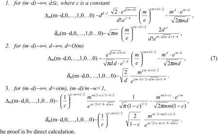
Proposition 5. Let ∆m(α1,…,αm)=| Ω(α1,…,αm) – Nm(α1,…,αm)|, δm(α1,…,αm)= Ω(α1,…,αm)/ Nm(α1,…,αm), m≥4. Then
1. for (m–d)→∞, d≤с, where с is a constant
∆m(m–d,0,…,1,0…0) ∼dd–1⋅ 1(/4 )
! 2
e d
e m d
⋅
⋅ − (m d)/2
e
m +
–
d m e md m d
π
2
−
⋅ ,
δm(m–d,0,…,1,0…0)∼ πm
2 / ) (m d
e
m −
4 / 1
! 2
+ − − m d m
d
e d
d
,
2. for (m–d)→∞, d→∞, d=O(m)
∆m(m–d,0,…,1,0…0) ∼ ( ) 1/4 e d d e m d d
⋅
+ −
π
2 / ) (m d
e
m +
–
d m e md m d
π
2
−
⋅ , (7)
δm(m–d,0,…,1,0…0)∼ d
2
4 / 1 2 / ) 5 (
2 / ) 1 (
+ − − −
+ −
d m m
d m
e m
. 3. for (m–d)→∞, d=o(m), (m–d)/m→c<1,
∆m(m–d,0,…,1,0…0)∼
2 / ) 1 (
1 ⋅ +
cm
c m mc
c m
e m
⋅ − +
− −
4 / 1 2 /
2 / 3 2 / ) 2 (
2 / 3
) 1 (
1
c −
π – 2 (1 )
) 1 (
c m m
e mm c cm
− ⋅ ⋅ −
π , δm(m–d,0,…,1,0…0)∼
2 / ) 1 (
1 ⋅ +
cm
c 1−c
2
c m m c m
c m m
e m
⋅ − + ⋅ +
− −
4 / 1 2 /
2 / ) 1 ( 2 /
. The proof is by direct calculation.
Let Ωm,d=Ω(m–d,0,…,1,0…0), Nm,d =Nm(m–d,0,…,1,0…0), Pm,d(t)=P{ρ(k)∈B(m–d,0,…, 1,
0…0 )}, Pm,d(p)= P{s∈B(m–d,0,…,1,0…0)}.
Table 2
The number of keys of RC4 generating the set of permutations with the cyclic structure {1m–d 20…d1…m0} for different m
m d Ωm,d Nm,d Pm,d(t) Pm,d(p)
5. Conclusion
In this paper we computed the number of keys of RC4 generating initial permutations with the same cyclic structure. We find that the distribution is not uniformly random and prove that the probability of generating the identical permutation is in π
4 / 1 2 / 3
2 / ) 1 (
+ −
+
m m
m
e m
more what you would expect. Therefore, to determine an initial permutation of RC4 we can do the following.
Let αr=(α1,…,αm) be a m-dimensional vector that coordinates are a solution of the equation
1α1+2α2+…+mαm=m.
I. Preliminary step.
a) Compute Ω(αr), Nm(αr), δm(αr)= Ω(αr)/ Nm(αr) for all solutions of the equation.
1α1+2α2+…+mαm=m.
b) On the set of vectors αr we define the order relation. We’ll suppose that αr≥αr′ if
δm(αr)≥δm(αr′) and αr1≥αr2≥αr3≥… if. αrr≥αrt for r≤t.
II.
Suppose Λ1(1)=∅, r=1.
j-step of testing.
1. Randomly from the set B(αrr)\ Λr(j) choose a permutation sr(j);
2. Suppose s0=sr(j);
3. Λr(j+1)= Λr(j)∪ sr(j);
4. For the state (0, 0, s0) compute L=3/2m keystreams z1*,…, zL*;
5. If zk=zk* for all k=1,L , then we find true the initial state. If there exist k∈{1 } such that ,L
zk≠zk*, then for Λr(j+1)= B(αrr) suppose r=r+1, Λr(j+1)= ∅ and go to step II; for B(αrr)\ Λr(j+1)≠∅ go to step 1.
6. Acknowledgment
The author would like to thank scientific adviser professor B. A. Pogorelov for help.
References
[1] Golic, J. D, Linear Statistical Weakness of Alleged RC4 Keystream Generator. Advances in Cryptology -- EUROCRYPT '97.
[2] Fluhrer S.R., McGrew D. A. “Statistical analysis of the alleged RC4 keystream generator”, Proceeding of FSE’2000, Springer-Verlag.
[3] Mantin I. Shamir A. “A practical attack on broadcast RC4”, Proceeding of FSE’2001, Springer-Verlag.
[4] Mister S., Tavares S., “Cryptanalysis of RC4-like ciphers”, Proceeding of SAC’98, Springer-Verlag.
[5] Knudsen L., Meier W., Preneel B., Rijmen V., Verdoolaege S, “Analysis method for (alleged) RC4”, Proceeding of ASIACRYPT’98, Springer-Verlag.
[6] Grosul A.L., Wallach D.S. “A related key cryptanalysis of RC4”, 2000, to appear.
[7] Pudovkina M. “Short cycles of the alleged RC4 keystream generator ”, 3nd International Workshop on Computer Science and Information Technologies, CSIT’2001, YFA, 2001.
[8] M. Pudovkina “Statistical weakness in the alleged RC4 keystream generator”, 4 International Workshop on Computer Science and Information Technologies, CSIT’2002, 2002.
Fig.1. P{ρ(k)∈ B(m–d,0,…0,1,0,…0)}= Ω(m–d,0,…0,1,0,…0) m
m
1
(the solid line) and P{s∈B(m–d,0,…0, 1,0, …0)} (the dashed line) if s is uniformly random for m=64.
1 10 100
1.10 88 1.10 87 1.10 86 1.10 85 1.10 84 1.10 83 1.10 82 1.10 81 1.10 80 1.10 79 1.10 78 1.10 77 1.10 76 1.10 75 1.10 74 1.10 73 1.10 72 1.10 71 1.10 70 1.10 69 1.10 68 1.10 67 1.10 66 1.10 65 1.10 64 1.10 63 1.10 62 1.10 61 1.10 60 1.10 59 1.10 58 1.10 57 1.10 56 1.10 55 1.10 54 1.10 53 1.10 52 1.10 51 1.10 50 1.10 49 1.10 48 1.10 47 1.10 46 1.10 45 1.10 44 1.10 43 1.10 42 1.10 41 1.10 40 1.10 39 1.10 38 1.10 37 1.10 36 1.10 35 1.10 34 1.10 33 1.10 32 1.10 31 1.10 30 1.10 29 1.10 28 1.10 27 1.10 26 1.10 25 1.10 24 1.10 23 1.10 22 1.10 21 1.10 20 1.10 19 1.10 18 1.10 17 1.10 16 1.10 15 1.10 14 1.10 13 1.10 12 1.10 11 11.10.1010
9
1.10 8 1.10 7 1.10 6 1.10 5 1.10 4 1.100.010.13 0.016
5.044 10× −88
P_RC4 64 t( , ) P_ter 64 t( , )
63