Copyright1998 by the Genetics Society of America
A Nonparametric Bootstrap Method for Testing Close Linkage vs. Pleiotropy
of Coincident Quantitative Trait Loci
Claude M. Lebreton,* Peter M. Visscher,
†Christopher S. Haley,
‡Andrei Semikhodskii*
,1and Steve A. Quarrie*
*John Innes Centre, Norwich NR4 7UH, United Kingdom,†Institute of Ecology and Resource Management, University of Edinburgh, Edinburgh EH9 3JG, United Kingdom and‡Roslin Institute, Edinburgh EH25 9PS, United Kingdom
Manuscript received December 30, 1997 Accepted for publication June 30, 1998
ABSTRACT
A novel method using the nonparametric bootstrap is proposed for testing whether a quantitative trait locus (QTL) at one chromosomal position could explain effects on two separate traits. If the single-QTL hypothesis is accepted, pleiotropy could explain the effect on two traits. If it is rejected, then the effects on two traits are due to linked QTLs. The method can be used in conjunction with several QTL mapping methods as long as they provide a straightforward estimate of the number of QTLs detectable from the data set. A selection step was introduced in the bootstrap procedure to reduce the conservativeness of the test of close linkage vs. pleiotropy, so that the erroneous rejection of the null hypothesis of pleiotropy only happens at a frequency equal to the nominal type I error risk specified by the user. The approach was assessed using computer simulations and proved to be relatively unbiased and robust over the range of genetic situations tested. An example of its application on a real data set from a saline stress experiment performed on a recombinant population of wheat (Triticum aestivum L.) doubled haploid lines is also provided.
T
HE gradual development of different types of mo- Roninet al. (1995) and Korolet al. (1995) used thelecular markers over the past decade has widened correlation between traits to increase the QTL detection the applicability of quantitative trait locus (QTL) map- power in experiments involving two traits with some ping to many species, even some for which variability correlation between them of genetic and/or environ-between lines is limited. Increased marker density has mental origin. In so doing, they assumed pleiotropy for facilitated accuracy of QTL positioning, which, in turn, every QTL mapped. In cases when this hypothesis was allows the development of comparative QTL mapping. wrong,JiangandZeng(1995) demonstrated that the
Comparisons of coincident associations of markers and estimates of the QTL effects and positions were biased. QTLs can take place between genomes of related genus While staying within the same framework, the latter within a family, a subfamily, or a tribe, thus exploiting authors extended the approach to the simultaneous the conserved synteny between genomes that may exist. analysis of more than two traits without having to assume It can also take place between different traits and across pleiotropy for every QTL being mapped. They termed different environments. their method “Joint Mapping.” They were then able to Among the different sorts of recombinant populations develop a test of close linkage vs. pleiotropy for a set derived from line crosses, doubled haploid and recom- of n QTLs, i.e., one QTL per trait detected in the same binant inbred lines are more amenable to comparative genomic region for the n traits. For two traits, the test QTL mapping between traits and between environ- statistic is the likelihood ratio
ments because the same genotypes can be used in
sev-LR252 ln(L20/L2), (1)
eral experiments. The experimental power is thus
in-creased because the different trait distributions are no where L
20 corresponds to the likelihood of the most
longer independent and can be studied as a multivariate likely full model, where the two QTLs are fitted without
z-dimensional distribution (where z is the number of any constraints. L
2is the likelihood of the model, where
traits or environments studied). Thus, as far as a QTL the two QTLs are fitted with the constraint that they comparison between traits is concerned, existing ge- must lie at the same position along the chromosome. netic and environmental correlations can be exploited. JiangandZeng(1995) suggest that this likelihood ratio asymptotically follows ax2distribution with 1 d.f. at the
null hypothesis of pleiotropy. In the context of the LOD
Corresponding author: Claude M. Lebreton, BIOCEM–Groupe Lima- support interval of a QTL’s position estimate, van
grain, 24, avenue des Landais, 63170 Aubie`re, France. Ooijen
(1992) andManginet al. (1994) demonstrated E-mail: [email protected]
that such ax2distribution no longer constituted a good
1Present address: School of Biological Sciences, University of
Man-chester, Manchester M13 9PT, UK. approximation of the real distribution of LR2when the
the putative QTL, they are slower than the multiple linear
QTL was of small or medium effect. We are not aware
regression, for example, as simplified by Whittakeret al.
that simulation studies have been performed to assess
(1996). Multiple linear regression constitutes an
approxima-the distribution of LR2over a range of situations, so it tion of the maximum likelihood-based interval mapping in
is possible that the same applies to this test of close that only the within-marker class distribution of the residuals
is considered and assumed normal (MartinezandCurnow
linkage vs. pleiotropy.
1992;Xu1995). However, the method gives almost identical
Visscheret al. (1996) proposed a less biased
alterna-results to those from the maximum likelihood-based methods
tive to the LOD support interval. They estimated
empiri-(HaleyandKnott1992).Wallinget al. (1998) could
never-cally a curve of probability density of the QTL’s position theless show, by using a large number of replicated simula-using the nonparametric bootstrap, in which the origi- tions, the existence of a small but significant bias that tends
to place the estimated QTL position closer to the nearest
nal data are resampled N times with replacement and
flanking marker. In this study we used two regression-based
then plotted the frequency of the different positions
QTL mapping methods for the assessment of the test of
link-observed. This procedure yielded confidence intervals
age vs. pleiotropy.
on the QTL’s position that performed better than LOD The first QTL mapping procedure was used in situations support intervals but tended to be too conservative when of saturated coverage of the genetic map with one marker
every centimorgan, to minimize any possible confounding
ef-the QTL accounted for,10% of the total trait variance.
fects due to the bias described above. Applying the principles Lebreton and Visscher (1998) managed to reduce
established by Stam (1991), Zeng (1993), Rodolphe and
the conservativeness and the size of the confidence
in-Lefort(1993), andWrightandMowers(1994), given the
tervals to a nearly unbiased level by conditioning the high and regular marker density over the genome, a simple bootstrap on the genetic model, provided there was no marker-regressor selection was implemented to identify the
QTLs. Because of their computational speed, regression
meth-bias on the QTL’s position estimate.
ods lend themselves to resampling schemes. The QTLs were
In this study, we have used the selective bootstrap
fitted at the positions of the selected markers, and therefore
concept to develop a novel method to test close linkage
there were as many QTLs declared as there were markers
vs. pleiotropy. In so doing, we replaced the likelihood selected. Their estimated additive effect was the partial
regres-ratio test statistic ofJiangandZeng(1995) by a confi- sion coefficient related to the corresponding
marker-regres-dence interval on the estimated distance between two sor. During the marker selection, a first, relatively lax, forward procedure, with an inclusion F-ratio of 4.0, adds a subset of
QTLs affecting different traits that are suspected to
cor-all the markers of the chromosome, some of which are
in-respond to the same locus (hypothesis of pleiotropy).
cluded by chance (as discussed by LebretonandVisscher
Our aim is to propose a test that is easy to implement 1998). Then, a stringent backward procedure was imple-and program (in the C-shell of a UNIX system, for mented to reject some markers. The stringency chosen deter-example) with a variety of QTL mapping methods. The mines the risk of type I error, i.e., the risk of retaining a false QTL. The stringent F-threshold is calculated empirically
test must also be as little biased as possible over a range
according to the protocol presented in Lebreton and
of genetic configurations commonly encountered. An
Visscher (1998) and follows the principles described by
absence of bias means that the null hypothesis is only
ChurchillandDoerge(1994).
rejected at the nominal frequency of type I error speci- The second QTL mapping procedure was applied in situa-fied by the user. The bias and the power of the method tions where the robustness of the test was assessed with
nonsat-urated marker coverage of the genome. In a first stage, a
are assessed by simulations using a range of genetic
subset of markers was chosen in the same way as the first
configurations. Finally, an example of its application to
method. Then, an “interpretation” stage followed, during
a real data set that comes from a saline stress experiment
which the number of QTLs and the sign of their additive
performed on a recombinant population of wheat (Triti- effect (for the doubled haploid populations simulated in the
cum aestivum L.) doubled haploid lines is presented. context of this study) were estimated. A selected isolated marker, i.e., a marker for which no adjacent markers were selected, was interpreted as evidence of a single QTL situated nearby. If two adjacent markers were selected with “apparent” MATERIALS AND METHODS
effects (i.e., the partial regression coefficient of the marker-regressor in the fitted multilinear model) of the same sign, a
QTL mapping procedures: The test of close linkage vs.
single QTL was assumed between the two markers. If the pleiotropy that we propose can be implemented for any QTL
“apparent” effects of the two selected adjacent markers were mapping method that lends itself to an easy QTL model
identi-of opposite signs, two QTLs were assumed nearby. In any case, fication. However, as the method is based upon resampling,
the sign of the QTL effects was inferred to be that of the the speed of the QTL mapping procedure is important in
allowing the assessment of the test on thousands of simulated respective linked markers. This procedure constitutes a mini-mum estimate of the number of QTLs, but regardless, no data sets. Interval mapping-based methods, such as the interval
mapping (stricto sensu) ofLanderandBotstein(1989), the linear method can fit more than one QTL per marker interval.
This estimate of the number of QTLs on the chromosome of composite interval mapping ofZeng(1993, 1994) andBasten
et al. (1996), or the multiple-QTL models ofJansen (1993) interest and the sign of their effect constitutes the basis on
which the bootstrapped sample is rejected or not, as will be andJansenandStam(1994) provide asymptotically unbiased
QTL parameter estimates due to the property of the maximum explained later. It is followed by a third stage, if the sample is retained, which consists of estimating the effect and position likelihood-based analysis. However, as these methods
imple-ment an iterative algorithm (the EM algorithm;Dempsteret of the QTLs within marker intervals. Thus, if an isolated
marker was selected in the first stage, both its flanking markers
al. 1977) that must perform several cycles to converge to an
marker that reduces the residual sum of squares the most is hence, in cases of poor experimental power, the span of a confidence interval on D could be larger than the chromo-retained. The most likely interval that contains the QTL is
thereby identified. The partial regression coefficients of the some length. Unlike inJiangandZeng(1995), QTL position
trait 2 and QTL position trait 1 were estimated independently flanking marker-regressors fitted one at a time are used to
estimate the QTL’s additive effect and position within the with our QTL mapping procedures. Note that, more generally, our nonparametric bootstrap test could be applied to the interval according to Equations 2 and 3, as presented in
LebretonandVisscher(1998): original data regardless of the QTL mapping procedure that
is implemented.
Dj,k51⁄4lnbj1121⁄4lnbj11⁄2Dj,j11 (2) In this article, for simplicity we considered only a population of doubled haploid lines. Thus, let Xn,m be the matrix
con-a5exp (1⁄
2lnbj11⁄2lnbj111Dj,j11). (3)
taining all the marker genotypes made of n row-vectors, n being the number of genotypes, and of m column-vectors, m
Dj,k is the estimated distance in centimorgans between the
marker on the left and the QTL; a is the estimated additive being the total number of markers covering the genome. Also, let Y1and Y2be the vectors containing the n phenotypic values effect of the QTL;bjandbj11are partial regression coefficients
of the trait phenotype on the marker-type, the markers j and for trait one and trait two, respectively. The marker and the phenotypic data for the two traits of an individual are
resam-j 11 being fitted in turn; and Dj,j11is the distance in
centi-morgans between the flanking markers ( j and j 11). pled jointly (xi,1, xi,2, . . . xi,m, y1,i, y2,i) and constitute one “resam-pleable” data point.
In the case when two adjacent markers are selected, with
apparent effects of the same sign, the most likely interval that As inLebretonandVisscher(1998), a selective
nonpara-metric bootstrap was compared to a nonselective one. With contains the QTL is de facto identified. One of the flanking
markers, say the one on the left of the interval, is removed, the selective scheme, after the QTL mapping procedure was applied to the resampled data set, the parameter estimates and the partial regression coefficient of the one on the right
is calculated. Then the two markers are swapped over in the contributed values to their estimated empirical distribution only if the QTL model, i.e., the number of QTLs and the sign model, and the partial regression coefficient of the marker
on the left is calculated. Then Equations 2 and 3 are applied to of their effects on the chromosome under study, conformed, for both traits, to those inferred from the original data set these coefficients. When the adjacent markers are of opposite
signs the QTLs are fitted at the respective marker loci, and (see Figure 1B). Data sets producing other outcomes were rejected, and the original data were resampled again until the apparent effects are retained as the estimate of the QTLs’
effects—this as an ad hoc compromise between bias in QTL N conforming outcomes were recorded. In the nonselective
parameter estimation and speed of computation. If x (x.2) bootstraps, the same number of QTLs as that observed in the adjacent markers were selected with “apparent” effects of the original data set was fitted whether they were significant or same sign, x21 QTLs in coupling would be assumed. How- not in every resampled data set. All of the QTLs contributed ever, our linear approximation was no longer able to estimate values to the estimated empirical distributions of the parame-the QTLs’ 2(x21) parameters (position and additive effect ters.Visscheret al. (1996) demonstrated that 150 bootstrap
for each QTL) because there were only x values (the partial samples gave a sufficiently low bootstrap resampling error regression coefficients) to solve a system of 2(x21) equations component (due to the limited number of resampled data with 2(x21) unknowns.Whittakeret al. (1996) also demon- sets as opposed to the error due to the limited size of the
strated the insolvability of this configuration when only the original data set itself;Efron andTibshirani1993). So we
markers’ “apparent” additive effects are available. Thus, com- retained that value for the assessment of our test.
pared to other regression-based QTL mapping methods that The general assessment protocol for our test:The aim of include other markers as background parameters so that the the protocol is to assess empirically the bias and the power of full model tested explains as much genetic variance as possible, our test by evaluating the frequency of rejection of the null such as MQTL (Tinker and Mather 1995), our method hypothesis of pleiotropy over many data sets that are the
real-should yield very similar results, with only a slightly lower QTL izations of a given genetic configuration. The protocol was detection power. This small decrease in QTL detection power largely inspired by that described inVisscheret al. (1996)
is due to the fact that the pairs of adjacent markers are not and is depicted in Figure 1A. In a real data set, it is trivial to systematically included in the compared models. say that the test of close linkage vs. pleiotropy would not be
The test of close linkage vs. pleiotropy:The principle of applied if either of the two QTLs tested did not show a signifi-the test consists of using bootstrap resampling to obtain an cant effect. This is why, in our simulations, a prior selection empirical estimate of the sampling distribution of the “dis- was made in the original data sets (which we call replicates tance” between the two QTLs—one per trait—that map in from now on) so that only the replicates that yielded the the same genomic region. Here we use the word distance in simulated number of QTLs and had effects of the right sign the loose sense because this quantity can actually take negative were kept. A genome-wise risk of 5% type I error in this prior values and is defined as selection was chosen to provide a stringency equal to what would realistically be applied in a real data set. Then the
d5QTL position trait 22QTL position trait 1, (4)
bootstrap test to be assessed was applied to each of these retained replicates with a specified risk of 5% type I error where QTL positions are measured in centimorgans from the
(risk of wrongly rejecting the null hypothesis of pleiotropy, leftmost marker on the chromosome. In the rest of this article,
as specified above) for all the simulations. The proportion of we shall use D as its estimate. For a chosen type I error X %
outcomes for which the null hypothesis was rejected consti-for our test, i.e., an X % risk of rejecting the null hypothesis
tuted either: (1) an estimate of the power of the test when a of pleiotropy when pleiotropy was nevertheless the real
con-situation of close linkage for the QTL pair studied was simu-figuration, a symmetrical X% confidence interval was
calcu-lated, or (2) an estimate of the frequency of type I errors lated by taking the lower and upper [(1002X )/2]th
percen-when pleiotropy was simulated, i.e., an estimate of the bias of tiles of the empirical distribution. If the interval did not
the method, because the unbiased expectation for this ob-contain the value “0,” this value was considered as an outlier
served value should be the X% that was used to define the to the distribution of d, and the null hypothesis of pleiotropy
confidence interval on the value of d. was rejected. It accrues from the definition of d that it could
Figure1.—Comparative diagram of the selective bootstrap test, assessed on simulated data (A) and applied on real data (B).
were made of one chromosome only, with a length of either per genotype were used. The NaCl experiment was started at the end of May and finished in August 1994. The Na2SO4 160 or 180 cM. Populations of doubled haploid lines of sizes
ranging between 100 and 200 lines were simulated, with one experiment was started on 11 January 1996 and finished in the middle of April 1996. Before sowing, seeds were soaked QTL per trait in general. Heritabilities were defined as the
ratio of the phenotypic variance of genetic origin between in water, in Petri dishes at 48overnight and then left at room temperature to germinate. When coleoptiles reached 1–2 mm, the line means over the total phenotypic variance between
the line means. The trait’s heritability was either 0.1 or 0.2. the seedlings were transferred to rockwool blocks. For the first 5 days, plants were grown in water that was then replaced Only the mean of each line was simulated. Three QTLs per
trait, on the same chromosome and in repulsion with a trait with “Sangral” nutrient medium. The nutrient medium was gradually salinized when leaf one was fully expanded to reach heritability of 0.6, were also simulated to assess the test in more
complex genetic configurations. No epistatic interactions were a final concentration of 200 mm· liter21 in NaCl and 100
mm· liter21in Na
2SO4, respectively. Both experiments were simulated. The residuals were normally distributed.
Application of the test to real data:A recombinant popula- performed in a greenhouse with a 16-hr day length. Daytime and nighttime temperatures were maintained at z208 and tion of 96 doubled haploid lines of bread wheat (T. aestivum
L.) was used for some QTL studies on abiotic stress resistance 158, respectively, and the air humidity was maintained at a level of 50–60%. Plants were harvested at maturity. The aver-byQuarrieet al. (1994). It is derived from the cross Chinese
Spring3SQ1, with Chinese Spring being the maternal parent. age spike length in the NaCl experiment and the length of leaf five in the Na2SO4experiment were then measured. The SQ1 is a sibling line at F7of the line 25/3/2 from the cross
Highbury3 TW269 and was selected for high abscisic acid data analysis was carried out on the means of each genotype. The genome was covered with 331 markers, mostly RFLPs production under drought conditions. It is also an early line
that flowersz25 days before Chinese Spring in the absence of and AFLPs, plus a few morphological markers including the
Vrn1 gene (Galibaet al. 1995). This is the main gene
control-vernalization. Chinese Spring is known for its relative salinity
tolerance. ling the vernalization requirements of European wheat
varie-ties. It was scored as days to ear emergence in unvernalized Physiological, biochemical, and yield traits were measured
on plants grown in a controlled environment and subjected plants. In our population, it produced a clear-cut segregation for the flowering time between the genotypes. Each of the 14 to saline stress treatments comparing NaCl and Na2SO4, in
markers on average. However, due to a lack of variability in P value calculated as twice the minimum percentage of
out-the D genome of T. aestivum L. as described byCadalen et comes with an estimated d either above or below zero. It al. (1997), we could place only 3.7 markers per D genome corresponds to the integrated area of the empirical
distribu-chromosome. tion’s tail beyond zero and is multiplied by two because our
The marker map was constructed using the software Map- test is two-tailed; it is the equality of a variable (d) to a specific maker (version 3.0b) with the Haldane mapping function. A value (zero) that is tested. Thus, P is the maximum risk of set of 21 nulli-tetrasomic lines, 1 for each chromosome, al- type I error one would need to adopt to be able to reject the lowed us to assign unambiguously from one to eight markers null hypothesis of pleiotropy.
to each chromosome as anchor points. Other markers were then grouped around these anchor points using a LOD thresh-old of 3.0 and a maximum recombination fraction of 0.3.
RESULTS Unlinked linkage blocks with anchor markers on the same
chromosome were then forced into one linkage group and Biases in conservativeness of the selective bootstrap: oriented relative to each other according to Gale et al.’s
Table 1 presents the results of a series of simulations
(1995) consensus map for the RFLP markers. Segregation
aimed at assessing the bias of the selective bootstrap
distortion of the marker genotypes was investigated using a
x2test with 1 d.f. The normality of the trait distribution among method to test close linkage vs. pleiotropy in a low the genotype means was checked using Shapiro and Wilk’s power experimental design (although the heritability
W-statistic (Royston1982). The QTLs were mapped, and the
of an individual QTL can reach 20%). Nine genetic
test of close linkage vs. pleiotropy was performed using the
configurations were explored. In all of them, only one
procedures described above that we implemented in a
pro-QTL was simulated per trait, for two traits, on a genome
gram in Fortran 90 (Ellis et al. 1994). No epistatic effects
were fitted. The F-significance thresholds to retain markers composed of a 180-cM-long chromosome. Because it
in the backward selection stage of the QTL mapping proce- was the bias that was being explored, the QTLs were dure were determined empirically using 1000 permutations simulated at the same position for both traits. The simu-as described inChurchillandDoerge(1994) to achieve a
lated values for the additive effects were equal to unity.
target risk of 10% type I error genome-wise. Then, if the QTL
The correlation between the residuals, i.e., the
environ-was isolated (i.e., no QTLs in the adjacent intervals), the
F-statistic of a QTL was calculated by comparing the full model, mental correlation between the traits, was equal to zero.
including the markers flanking the QTL, to the reduced one Replicates were created until 2000 had been retained that did not contain them. Otherwise, if the QTL was fitted that conformed to the model simulated. For example, at the marker position in the specific cases described above,
when a QTL of 10% heritability was simulated for both
only this marker was removed from the full model to calculate
traits, 2260 replicates on average were generated to
re-the F-statistic.
The output of our test of close linkage vs. pleiotropy was a tain 1000 of them. The total number of replicates fell
TABLE 1
Frequencies of nonrejection of the null hypothesis of pleiotropy and sizes of the confidence intervals of the estimated distance between two QTLs for pleiotropic QTLs
Select (20 cM) Select saturated Nonselect
No. Pos A Pos B H2A H2B P (95%) CI size P (95%) CI size P (95%) CI size
1 90 90 10 10 97.7 102.84 95.7 113.7 99.2 146.0
2 15 15 10 10 96.4 114.83 96.1 121.2 98.8 195.8
3 5 5 10 10 94.0 108.7 95.8 126.9 98.5 210.9
4 5 5 10 20 88.4a 87.24 92.2a 98.2 96.6a 165.8
5 90 90 10 20 95.6 91.22 97.8 96.9 98.8 121.8
6 5 5 20 20 95.8 71.48 92.2 67.7 92.3 123.5
7 90 90 20 20 96.2 62.94 96.3 74.5 97.9 91.4
8 5 5 15 7.5 93.2a 110.3 94.6a 117.1 97.6a 198.3
9 90 90 15 7.5 94.4 103.8 96.0 110.4 99.2 139.7
No., number of the genetic configurations simulated; Pos A, position of QTL for trait A in centimorgans from the leftmost marker; Pos B, position of QTL for trait B in centimorgans from the leftmost marker; H2A, heritability of trait A; H2B, heritability of trait B; Select (20 cM), selective bootstrap with one marker every 20 cM; Select saturated, selective bootstrap with one marker every centimorgan; Nonselect, nonselective bootstrap with one marker every centimorgan; P (95%), frequency (percentage) of nonrejection of the null hypothesis (pleiotropy), using 95% confidence intervals on the estimated difference (QTL position trait B2QTL position trait A); CI size, average width of the 95% confidence intervals, in centimorgans. Both P (95%) and CI size were estimated over 2000 selected replicates. The simulated populations were made of 100 doubled-haploid lines. Five percent is the theoretical (expected) frequency of type 1 errors, and a significant departure of the
P (95%) observed frequency from the nominal 95% indicates a bias of the test in the particular configuration. aConfigurations for which there is a significant bias in the estimate of the difference (QTL position trait B
to 1200 when a QTL of 20% heritability was simulated distance between the two tested QTLs vary from more than 210 cM in the least powerful design toz90 cM in for both traits (results not shown). A saturated marker
coverage of one marker every centimorgan was com- the most powerful of the simulated set, with the nonse-lective scheme. They can be reduced to about 125 and pared to a density of only one marker every 20 cM.
The percentage estimates of inclusion of the value 67 cM, respectively, with the selective scheme. These confidence interval widths were estimated within confi-“0” by the 95% confidence intervals for the estimate of
d were within confidence limits of61.3%. The estimates dence margins of61 cM only. Thus, the greatest reduc-tion in confidence interval size is achieved for the least of the QTL additive effects were significantly biased
upward due to the selection of the replicates and then powerful designs, which makes sense, because a greater proportion of bootstrap samples were then rejected with of the bootstrapped samples. This bias is very small for
QTL heritabilities of 20%: 15.6% 6 2% on average the selective bootstrap.
Figure 2 illustrates the effect of the selection step in over the replicates and19.5%6 2% on average over
the bootstrap samples, for both marker densities. For the bootstrap resampling, where two QTLs at different positions were simulated. It appears that the selection, a heritability as low as 7.5%, the bias became more
important:133%62% on average over the replicates in addition to reducing the bias of the test, quite dramat-ically increases its power, especially when the heritability and149%62% on average over the bootstrap samples
with the dense marker coverage (results not shown). is low. However, heritabilities as low as 10% offer limited resolution in the population we studied because, even Biases were significantly higher with the sparse coverage
of one marker every 20 cM:140%63% and158%6 when the QTLs are 180 cM apart, the power of the selective bootstrap test reached only 88.4%.
2%, respectively.
Overall, the percentages of inclusion of the value “0” Effect of the marker density on the power of the test:
In Figure 3, three marker densities were tested for two were quite close to their expected values (95%), which
demonstrates the small bias of the method. The method population sizes—100 and 200 genotypes. The results demonstrated that a higher marker density significantly was even unbiased when the QTLs were as close as 5
cM to a chromosome end, because 95.8% of the 95% increased the resolution of the test for both sizes. For a population size of 100 genotypes, a difference of 10– confidence intervals contained the value “0” for a QTL
with a heritability of 10% with the dense marker cover- 15% in power of the test was consistently observed be-tween a sparse coverage of one marker every 20 cM and age and 94% with the sparse coverage (configuration 3
in Table 1). This last result contrasts with the properties a saturated coverage of one marker every centimorgan, over the different distances between the QTLs. With of the confidence interval on a QTL’s position,
calcu-lated using the same selective bootstrap, in which case the higher QTL detection power provided by the larger population size of 200, an even larger difference in QTL it is anticonservative when the QTL is close to a
chromo-some end, as demonstrated byLebretonandVisscher separation power was observed between the different
marker densities. (1998). Only when the heritabilities of the two QTLs
tested differed markedly, as in configuration 4 in Table Effect of the environmental correlation between the
traits on the power of the test:In Figure 4, the results
1, was the estimate of the “distance” significantly bi-ased—by about 5 cM—for both marker densities. Even then, there was not a big discrepancy between the ob-served and the expected percentages of inclusions with the tight marker coverage. However, the bias was more important with the sparse coverage.
Selective vs. nonselective bootstrap: In Table 1, the
selective bootstrap was also compared to the nonselec-tive one. The 95% confidence intervals obtained with the nonselective bootstrap appeared consistently con-servative, even very conservative when the QTLs were centrally situated (99.2%) in configuration 1. This im-plies that the hypothesis of pleiotropy is rejected too infrequently and therefore that the power of the test of close linkage vs. pleiotropy is not maximized with the
nonselective scheme. The only configuration for which Figure2.—Comparison of the power of the test with the
selective and the nonselective bootstrap methods, across a
the confidence intervals were not too large was one in
range of distances (d) between the two QTLs, for two different
which two QTLs of high heritability (20%) were
simu-heritabilities. The genome map was saturated with one marker
lated near a telomere. The method was rather
anticons-every centimorgan. The simulated population size was 100.
ervative, and the percentage of inclusion did not differ The chromosome length was 180 cM. Powers were estimated much from that obtained using the selective bootstrap. over 500 replicates for each configuration. r e is the
environ-mental correlation between the traits.
of d, the distance between the two QTLs, when r had a high absolute value. For r50, the average width of the 95% confidence interval of d was 77 cM but only 64 cM for r50.9 (results not shown).
Results presented in Figure 5 explore the effect of the environmental correlation in a less powerful design. The simulations followed the same protocol as that in Figure 4, and the population size was also the same, but the heritabilities of both traits were only 0.1. The maximum absolute value of r was also increased to 0.95 to accentuate any possible effect of this parameter. A very different pattern for the effect of r was observed.
Figure3.—Comparison of the power of the test across three
First, it was very asymmetrical around the value zero.
marker densities and two population sizes, over a range of
Negative values of r dramatically increased the power
distances between the two QTLs. Only the selective bootstrap
of the test, unlike positive values. Surprisingly, the lower
was applied. The powers were estimated over 500 replicates
density of one marker every 20 cM provided a slightly
for each configuration. The simulated population sizes were
100 and 200, and the correlation coefficient between the resid- better resolution except when r 5 0.45. The average uals was 0.45. The chromosome length was 180 cM. Both trait widths of the 95% confidence interval of d varied sig-heritabilities were 0.2.
nificantly between the different simulated configura-tions, from 11265 cM when r50 to 9766 cM when
r5 20.95, for a marker spacing of 20 cM. Besides the of a series of simulations, where different degrees of
differences in the size of the confidence interval of d, environmental correlation were combined with
differ-a bidiffer-as in the estimdiffer-ate of d seemed to further exdiffer-acerbdiffer-ate ent marker spacings, are plotted. The population size
the difference in power associated with r. Thus, in Table was 100, the trait heritability was 0.2, and the effect of
2, this bias was studied further. The average observed the environmental correlation was symmetrical around
value of d was calculated over 2000 retained replicates the value zero. The power of the test increased with a
and for the same range of genetic configurations as that high absolute value of the environmental correlation
simulated in Figures 4 and 5. Biases were significant (r). The effect of an increase in r was more pronounced
only with the lower simulated trait heritability of 0.1 for tight marker coverage than for loose marker
cover-and larger with the lower marker density of one every age. Thus, with one marker every 20 cM, we observed
20 cM. A negative value for r tended to bias the estimate an increase of only 5% in the power of the test between
of d upward (17.2 cM for r5 20.95 and one marker
r50 and r50.9, whereas with one marker every
centi-every 20 cM) and a positive value, downward (26.9 cM morgan the increase was 20%. This increase was
ex-for r 5 0.95 and one marker every 20 cM). Likewise, plained by a smaller confidence interval on the estimate
Figure4.—Comparison of the power of the test across five Figure5.—Comparison of the power of the test across five
values for the environmental correlation and three marker values for the environmental correlation and three marker
densities, for a distance of 40 cM between the two tested QTLs densities, for a distance of 40 cM between the two tested QTLs and trait heritabilities of 0.1. Only the selective bootstrap was and trait heritabilities of 0.2. Only the selective bootstrap was
applied. The powers were estimated over 500 replicates for applied. The powers were estimated over 500 replicates for each configuration. The chromosome length was 180 cM. The each configuration. The chromosome length was 180 cM. The
TABLE 2 mate of the distance between QTL 1 and QTL 2 was very slightly biased upward by 1.6 cM and that between
Average estimated distance between QTL for trait B
QTL 3 and QTL 4 was biased downward byz4–5.6 cM,
and QTL for trait A for linked QTLs
depending on the simulated position of QTL 5. The null hypothesis of pleiotropy, for QTL 5, was rejected
Marker
h2 r
e spacing (cM) D sD rpos with varying frequencies, from 3.6%, when the QTL was
simulated in the middle of the interval, to 9.8% when
0.2 20.9 10 39.8 0.30 0.011 NS
it was simulated at only 2 cM away from the flanking
20 40.6 0.36 20.014 NS
marker on the left. Simulations with the saturated map
0.0 10 39.7 0.30 0.0
20 39.6 0.36 0.0 showed biases in the same directions as those observed
10.9 10 39.7 0.30 20.027 NS with one marker every 20 cM for the three positions of
20 38.6 0.34 20.02 NS QTL 5, respectively (results not shown). This indicates 0.1 20.95 10 43.6 0.52 20.146*** not only that the biases observed for QTL 5 are due to
20 47.2 0.55 20.093***
the within-marker interval bias on QTL position
esti-0.0 10 37.8 0.57 0.0
mates but also that the linkage with other strong effect
20 39.2 0.59 0.0
QTLs differing for the two tested QTLs tends to affect
10.95 10 36.0 0.49 0.242***
20 33.1 0.53 0.205*** the estimated distribution of d and the conservativeness of the test. The power of the test was relatively low for
h2, heritability of the trait; r
e, simulated correlation
coeffi-the ocoeffi-ther two pairs of nonpleiotropic QTLs. It ranged
cient between the residuals; D, average estimated distance
from only 4.2 to 7.2%, for QTL 3 and QTL 4, which
between the QTL for trait A and the QTL for trait B;sD,
standard error of the mean; rpos, correlation coefficient be- were 8 cM apart, depending on the simulated position tween QTL position estimates; NS, nonsignificant correlation; of the linked QTL 5. The power of the test for QTL 1 ***, significant at a risk of type I error,0.001. The simulated and QTL 2 was not affected by the position of QTL 5 distance between the QTL for trait A and the QTL for trait
and was z44%.
B was 40 cM.
Application of the test to real data:There was a
sig-nificant difference between the parents for the length of leaf five. For Chinese Spring the value was 338.0 mm the correlation coefficients between the QTL position
estimates were only significant with the lower simulated on average and for SQ1 was 214.5 mm. The distribution of this trait among the recombinant genotypes did not trait heritability of 0.1, but with both marker densities.
A negative correlation between the residuals of the phe- differ significantly from normality. The intensity of the stress generated by Na2SO4 reduced the number of
notypic trait values generated a negative correlation
be-tween the QTL position estimates and vice versa. spikes to fewer than one per plant. SQ1 produced on average one spike per plant, whereas Chinese Spring
Behavior of the method in more complex genetic
situations:The power and the bias of the test were also did not produce any spikes in any plant. Twenty-three
genotypes did not produce any spikes at all. This gener-investigated in more complex configurations of several
QTLs per trait. The model was three QTLs per trait, on ated as many missing data for the average spike length trait. However, the distribution of the mean values of the a 160-cM-long chromosome. The QTLs were of equal
effect and linked in repulsion. Both trait heritabilities remaining genotypes did not differ significantly from normality.
were 0.6, and the residuals were correlated with r50.2.
The population was made of 150 doubled haploid lines. Segregation distortion in the marker genotypes was observed on 11 chromosomes, representing every ho-One thousand replicates were simulated. The results
are summarized in Table 3. QTLs 1, 3, and 5 affected moeologous group except group 6. In particular, chro-mosome 7A showed some segregation distortion in sev-trait 1, whereas QTLs 2, 4, and 5 affected sev-trait 2. Thus,
QTL 5 was pleiotropic by definition, and we had two eral regions. Markers at the telomeric end of the short arm of chromosome 5A, i.e., the two leftmost markers testable pairs of QTLs: QTLs 1 and 2 in one region of
the chromosome and QTLs 3 and 4 in another region. on our map, showed significant segregation distortion (P,0.001) in favor of the Chinese Spring-type alleles in The QTLs were 13 cM apart for the first pair and only
8 cM apart for the second pair. This design was inspired a 72:28 ratio. A relatively good correlation was observed between the lines’ phenotypic means for the two traits partly by that ofJiangandZeng(1995), although they
simulated F2populations. The simulated chromosome (R25 0.3, results not shown).
The detected QTLs for the two traits are listed in was covered with only one marker every 20 cM to assess
the robustness of the test in a realistic configuration. Table 4. The 1000 permutations determined an F-sig-nificance threshold of 13.35 for spike length and 12.87 Both testable pairs of QTLs in close linkage were
situ-ated in the same marker interval. QTL 5 was the only for leaf length. Four QTLs were detected for spike length and these accounted for 58% of the phenotypic QTL in its interval and was separated from the nearest
esti-TABLE 3
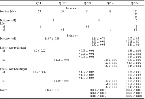
Parameters of QTL positions and effects and their estimates for data sets with three QTLs affecting each trait
QTL1 QTL2 QTL3 QTL4 QTL5
Parameters
Position (cM) 23 36 81 89 127
122 130
Distance (cM) 13 8 0
Effect
a1 1 21 1
a2 21 1 21
Estimates
Distance (cM) 14.6760.66 4.1460.70 0.0760.5
3.9060.60 20.1160.3
2.5260.66 2.4460.9
Effect (over replicates)
a1 1.060.02 20.9560.02 1.3660.06
20.9560.02 0.9860.02
20.9560.02 1.5460.06
a2 21.0660.03 1.4860.06 21.6360.06
1.5260.06 21.560.06 1.3260.06 21.4560.03 Effect (over bootstraps)
a1 1.1560.02 21.0260.02 1.3660.04
21.0660.02 1.1060.02
21.0360.02 1.4760.04
a2 21.1960.02 1.4760.04 21.5860.04
1.5460.04 21.5460.04 1.3760.04 21.4560.04
Power 0.44460.031 0.06660.015 0.05460.013
0.07660.016 0.09860.018 0.04260.012 0.02260.004
Position (cM), position of the QTLs in centimorgans from the leftmost marker, on the unique chromosome; Distance (cM), difference (QTL position trait 22QTL position trait 1) for a pair of QTLs testable for pleiotropy vs. close linkage; a1, additive effect of the QTLs affecting trait 1, with its 95% confidence limits; a2, additive effect of the QTLs affecting trait 2, with its 95% confidence limits. Power, for QTLs 1–4: power of the test of close linkage vs. pleiotropy, i.e., frequency at which the null hypothesis of pleiotropy is rejected for a nominal risk of type I error of 5%; for QTL 5, percentage of type I error for a nominal risk of 5%.
The trait heritabilities are 0.6, the population size is 150, and the environmental correlation coefficient between the traits is 0.2. The chromosome is 160 cM long and covered with one marker every 20 cM. For QTL 5, three positions were simulated, and the three respective percentages of type I errors are listed bottom right. The corresponding powers of the test for QTLs 3 and 4 are also detailed. QTLs 1, 3, and 5 affect trait 1. QTLs 2, 4, and 5 affect trait 2. QTL 5 is therefore the only pleiotropic QTL.
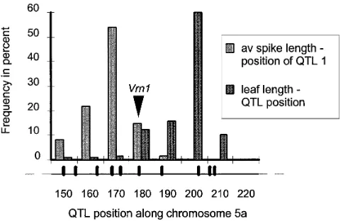
significant (F 5 44.8) and was estimated at 168.8 cM Only one QTL was detected for leaf length in the ge-nome scan and this was at 202.6 cM on 5A, z20 cM from the leftmost marker on our map. It is close to
Vrn1, which mapped at 179.1 cM. The empirical distri- from Vrn1, which required too high a risk of type I error (7%) to be rejected as its candidate gene. Figure 6 shows bution of its position estimate, using the selective
boot-strap procedure described inLebretonandVisscher the comparative empirical distributions of the first
QTL’s position for the spike length and that of the QTL (1998), did not allow us to reject Vrn1 as its candidate
gene. One would have had to adopt a 26% type I error for the leaf length on 5A. Applying our test of close linkage vs. pleiotropy to these two QTLs that mapped risk for this rejection (results not shown elsewhere).
The second QTL on 5A for this trait mapped in a poorly near Vrn1 showed that the hypothesis of pleiotropy could be rejected with a stringency that allowed a 1% covered region of the chromosome at position 229.0
cM in a 34.2-cM-wide marker interval and was linked in type I error risk. Figure 7 shows the empirical distribu-tion of D, and zero clearly appears as an outlier to repulsion with the first QTL. Vrn1 could be rejected as
its candidate gene with a 1% type I error risk, again using the distribution. Figure 8 shows that the correlation between the two QTLs’ estimated positions was not at
TABLE 4
List of the QTLs detected for the average spike length and the leaf length characters
Chromosome QTL no. Position Effect F
Average spike length (adjusted R250.58)
5a 1 168.8 0.59 44.80
5a 2 229.0 20.60 32.56
5b 1 0.7 0.31 19.81
7a 1 414.39a 0.27 16.41
Leaf length (adjusted R250.34)
5a 1 202.6 239.08 48.15
Chromosome, name of the chromosome on which the QTL was detected; QTL no., order of the QTL on the particular chromosome; position, estimated distance in centimorgans from the leftmost marker on the chromosome; effect, estimated effect of the QTL; F, F-statistic of the QTL.
aThe total genetic length is likely to be grossly overestimated due to some wide gaps between several linking blocks on this chromosome.
all significant. The test was also applied to the second The QTL mapping method:Although the estimation of our QTL effect and position used the information QTL on 5A for the spike length, despite the poor marker
coverage in its proximity, and to the QTL for the leaf from both flanking markers, the detection of the QTLs was carried out by selecting individual markers as op-length. Figure 9 shows the comparative distributions of
these two QTLs’ position estimates. Figure 10 shows the posed to testing pairs of adjacent markers as in the interval mapping or its multiple-linear approximations empirical distribution of D for this test.
(Haley and Knott 1992). However, the consequent
loss of power in our configurations with one marker
DISCUSSION every 20 cM is not very high, as shown byKnottand Haley(1992) andRebaiet al. (1995).
We have introduced a novel way of testing close
link-The selective bootstrap: The selection step inserted
age vs. pleiotropy. Our method is based upon the
empir-in the bootstrap resamplempir-ing scheme was identical to that ical distribution of the distance between QTLs mapped
described inLebretonandVisscher(1998). Because a
for different traits in the same chromosome region. The
significance threshold greater than zero was imposed method is very easy to implement and does not make
to retain a QTL when analyzing an original data set, it any assumptions about the distribution of data or test
was reasonable to apply the same threshold in order to statistics. Over the range of configurations tested with
follow the same procedure when analyzing the boot-one QTL per chromosome, the method presented little
bias, in that under the null hypothesis of pleiotropy the proportion of nonrejection was close to its expected value.
Figure7.—Empirical distribution of the distance between
the two QTLs of the first pair tested for close linkage vs.
Figure6.—Comparative empirical distributions of the
esti-mated QTL positions obtained from 200 selective bootstraps pleiotropy, obtained from 200 joint resamplings of the original data, using the selective bootstrap method. D is the estimated applied on the original data, for the first pair of QTLs tested
strapped data sets to work out the empirical distribution and, as observed in our simulations, the estimated dis-tance could differ significantly from zero. Even then, of our d statistic (seeEfronandTibshirani1993). This
means that we only retained the bootstrap outcomes the conservativeness of the test did not seem overly decreased, which demonstrates the general robustness that showed the same QTLs for both traits. Selection was
also imposed on the sign of the QTLs. This is because a of the method.
Concerning the biases observed in the estimates of confidence interval on a QTL’s parameter is defined
on the condition that this QTL exists. In other words, the QTL effects after the two selection stages, they are not solely an artificial consequence of the experimental there is a genetic factor present somewhere along the
chromosome, acting in a given direction on the trait. protocol to assess our bootstrap method, but corre-spond to what would be observed when a set of real A QTL detected with an effect of opposite sign violates
this condition and cannot logically be retained to con- data is analyzed. Indeed, regarding the bias due to the tribute a value to the estimate of the statistic’s empirical first selection, if a pair of QTLs is to be tested for close distribution. Nevertheless, the selection step generates linkage vs. pleiotropy, their observed effects would have an upward bias in the absolute value of the estimated to be significant for the QTLs to be detected in the first QTL effect. As QTLs of higher effects have smaller con- place. Imposing a significance threshold on the QTL fidence intervals on their position estimate, a prerequi- effect for their detection involves a bias on their esti-site of the bootstrap is violated, namely that the statistic mated effects, as investigated byHyneet al. (1995). As
estimated from the bootstrapped data follows the same for the bias due to the selection stage introduced in the distribution law as that estimated from the original data bootstrap resampling, it grows with the percentage of set. Because we did not find the means to solve the issue outcomes rejected, which is inversely related to the size analytically, we resorted to simulations. of the QTL effects.
In contrast to the situation in which the bootstrap Effect of the environmental correlation and of the
resampling was applied on a single QTL’s position, as marker spacing: We observed that the environmental in Lebreton andVisscher(1998) when the distance correlation had a different pattern of effect, depending
between two QTLs was resampled, in this study, no bias on the heritability of the traits. Thus, when the heritabil-was observed when the pleiotropic QTL heritabil-was situated ity was such that the experimental power was high near a telomere, provided that the percentages of vari- (power of the test of close linkage vs. pleiotropy.50%), ance that it accounts for are similar for both traits. In then the resolution power of our test also increased other words, on average, the distance is close to zero. significantly with a high absolute value of the environ-Yet the individual estimated QTL’s positions were biased mental correlation r. This increase in resolution and toward the middle of the chromosome, as investigated the resolution of the test itself were greater with a higher byHyneet al. (1995). The fact that two QTLs of similar marker density. When the traits’ heritability was lower,
significance, at the same position, are subject to similar a totally different pattern emerged. The effect of r was biases may explain why their estimated distance re- no longer symmetrical around the value zero, and it mained close to the expected value of zero. Conversely, was the less dense marker density that provided a slightly if a pleiotropic QTL explained a markedly different higher resolution power of the test. When the heritabil-proportion of the variance of the two traits, the biases in
the two estimated QTL positions would also be different
Figure9.—Comparative empirical distributions of the esti-Figure 8.—Fitted regression between the estimated QTL
positions of the first pair of QTLs tested for close linkage mated QTL positions obtained from 200 selective bootstraps applied on the original data, for the second pair of tested
vs. pleiotropy, over the joint resamplings from the selective
gain in resolution obtainable from the correlation of the environmental residuals.
In the absence of bias on the QTL position estimates, the test of close linkage vs. pleiotropy showed very little bias itself. It also turned out to be robust in the presence of such biases on the QTL position estimates, whether they were due to differences between the two traits’ heritabilities or to linkage with other QTLs at different distances as in the example presented in Table 3, pro-vided that the marker density was high. However, when the marker density decreased, the test became more sensitive to these biases, including the within-marker interval bias on QTL position estimate.
Analysis of the wheat data set: The population sizes
were small because data for a maximum of 96 doubled haploid lines were present in the data set. However, the
Figure10.—Empirical distribution of the distance between
high heritabilities of the traits studied compensated for
the two tested QTLs of the second pair tested for close linkage
the small sizes of our sample. The relevant chromosome
vs. pleiotropy, obtained from 200 joint resamplings of the
span was covered with one marker every 6 cM on average
original data, using the selective bootstrap method. D is the
estimated distance between the two QTLs. for the first pair of QTLs tested for close linkage vs. pleiotropy, which mapped at some 34 cM away from each other. This allowed us to separate them with a ity was lower, the residuals represented a higher part maximum 1% type I error risk. The risk of type I error of the phenotypic variation. Thus a strong correlation at which the second QTL for the spike length on chro-between the residuals such as those observed byChev- mosome 5A can be separated from the QTL of leaf erudet al. (1997), for example, can have a dramatic length is to be considered with caution because of the
effect on the resolution power as our simulations poor marker coverage around the former. Because our showed. The direction and magnitude of this effect are QTL mapping method fitted all the detectable QTLs hard to predict intuitively. We observed that a positive on all the chromosomes, in the full model, no residual
r generated a positive correlation of the QTL position correlation of genetic origin was left. There was no
estimates between the two traits. This is expected to correlation of environmental origin between the residu-decrease the variance of D and therefore increase the als because the data came from two separate experi-power of the test. A negative r generates a negative ments for the two traits. As a consequence, there was correlation of the QTL position estimates between the also no correlation between the reestimated QTL posi-two traits. This is expected to increase the variance of tions and no extra power to be gained from a joint
D and therefore decrease the power of the test. However, resampling of the data in this particular case. More
we also showed empirically that a positive r also gener- generally, for traits measured on the same individuals ates a downward bias of D, which, if no other effects (as opposed to the case presented above), when imple-were present, would increase the apparent separation menting a QTL mapping method that includes all the power of the test and vice versa. The overall effect is detectable genetic effects in its full model, such as the thus difficult to predict, and the simulations showed composite interval mapping of Zeng(1993, 1994) or
that the negative correlation between the residuals had the multiple-QTL model ofJansen(1993), we also
ex-the greatest effect in increasing ex-the resolution; ex-there- pect little extra power to be drawn from a joint resam-fore, the bias on the QTL position estimates had the pling of the data if the correlation of environmental prevailing effect. origin between the traits is low. However, in this config-It also appears that the correlation between the envi- uration, the nonselective bootstrap method still has the ronmental residuals of the two traits studied could not merit of supplying an assumption-free nonparametric increase the resolution beyond a certain limit despite test that is robust in a variety of situations.
analysis: unreliability and bias in estimation procedures. Mol.
of implementation in software using any QTL mapping
Breeding 1: 273–282.
method, provided the mapping method lends itself to Jansen, R. C.,1993 Interval mapping of multiple quantitative trait loci. Genetics 135: 205–211.
the easy and quick estimation of the minimum number
Jansen, R. C.,andP. Stam,1994 High resolution of quantitative
of QTLs along the chromosome of interest. It can be
traits into multiple loci via interval mapping. Genetics 136: 1447–
applied to the multiple-trait joint composite interval 1455.
Jiang, C.,and Z.-B. Zeng,1995 Multiple trait analysis of genetic
mapping ofJiangandZeng(1995) through resampling
mapping for quantitative trait loci. Genetics 140: 1111–1127.
of the estimated distance between the two QTLs of
inter-Kearsey, M. J.,andH. S. Pooni,1996 The Genetical Analysis of
Quanti-est in the unconstrained full model, thereby taking ad- tative Traits. Chapman & Hall, London.
Knott, S. A.,andC. S. Haley,1992 Aspects of maximum likelihood
vantage of the increased QTL detection power of their
methods for the mapping of quantitative trait loci in line crosses.
QTL mapping method. It is unlikely that our test brings Genet. Res. 60: 139–151.
any increase in separation power to the likelihood ratio- Korol, A. B., I. Y. RoninandV. M. Kirzhner,1995 Interval mapping of quantitative trait loci employing correlated trait complexes.
based test, but it is unlikely that any analytical method
Genetics 140: 1137–1147.
would bring the resolution of the test below 10–30 cM Lander, E. S.,andD. Botstein,1989 Mapping mendelian factors underlying quantitative traits using RFLP linkage maps. Genetics
in common QTL mapping designs with realistic
popula-121:184–199.
tion sizes (KearseyandPooni1996). To go below that
Lebreton, C. M.,andP. M. Visscher,1998 Empirical
non-paramet-resolution it will be necessary to resort to fine QTL ric bootstrap strategies in QTL mapping: conditioning on the genetic model. Genetics 148: 525–535.
mapping designs, such as advanced intercross lines or
Mangin, B., B. GoffinetandA. Rebai,1994 Constructing
confi-near-congenic lines, or to greatly increased population
dence intervals for QTL location. Genetics 138: 1301–1308.
sizes. Martinez, O.,andR. N. Curnow, 1992 Estimating the locations and the sizes of the effects of quantitative trait loci using flanking We express our gratitude to M. J. Kearsey, J. W. Snape, and markers. Theor. Appl. Genet. 85: 480–488.
J. K. M. Brown for their helpful comments on the manuscript. C.S.H. Quarrie, S. A., M. Gulli, C. Calestani, A. SteedandN. Marmiroli, is grateful to Ministry of Agriculture, Fisheries and Food (MAFF) and 1994 Location of a gene regulating drought-induced abscisic Biotechnology and Biological Sciences Research Council (BBSRC) acid production on the long arm of chromosome 5A of wheat.
Theor. Appl. Genet. 90: 1174–1179. for financial support. Finally, we are also grateful to the John Innes
Rebai, A., B. GoffinetandB. Mangin,1995 Comparing power of Foundation and Monsanto who funded the Ph.D. project of the
corre-different methods for QTL detection. Biometrics 51: 87–99. sponding author.
Rodolphe, F.,andM. Lefort,1993 A multi-marker model for de-tecting chromosomal segments displaying QTL activity. Genetics
134:1277–1288.
Ronin, Y. I., V. M. KirzhnerandA. B. Korol,1995 Linkage between loci of quantitative traits and marker loci: multi-trait analysis with LITERATURE CITED
a single marker. Theor. Appl. Genet. 90: 776–786.
Basten, C. J., Z.-B. ZengandB. S. Weir,1996 QTLCartographer: Royston, J. P.,1982 Algorithm AS181: The W test for normality. a suite of programs for mapping quantitative trait loci, p. 108 in Appl. Stat. 31: 176–180.
Abstracts to Plant Genome IV. Academic Press, San Diego. Stam, P.,1991 Some aspects of QTL mapping. Proceedings of the
Eighth Meeting of the Eucarpia Section Biometrics in Plant Cadalen, T., C. Boeuf, S. Bernard and M.Bernard, 1997 An
Breeding, Brno, Czechoslovakia, pp. 23–32. intervarietal molecular map in Triticum aestivum L. Em. Thell.
Tinker, N. A.,andD. E. Mather,1995 MQTL: software for simpli-and comparison with a map from a wide cross. Theor. Appl.
fied composite interval mapping of QTL in multiple environ-Genet. 94: 367–377.
ments. J. Quant. Trait Loci. Avail. World Wide Web: http://probe. Cheverud, J. M., E. J. RoutmanandD. J. Irschick,1997 Pleiotropic
nalusda.gov:8000/otherdocs/jqtl/jqtl1995-02/jqtl16r2.html/. effects of individual gene loci on mandibular morphology.
Evolu-van Ooijen, J. W.,1992 Accuracy of mapping quantitative trait loci tion 51: 2006–2016.
in autogamous species. Theor. Appl. Genet. 84: 803–811. Churchill, G. A.,and R. W.Doerge,1994 Empirical threshold
Visscher, P. M., R. ThompsonandC. S. Haley,1996 Confidence values for quantitative trait mapping. Genetics 138: 963–971.
intervals in QTL mapping by bootstrapping. Genetics 143: 1013– Dempster, A. P., N. M. LairdandD. B. Rubin,1977 Maximum
1020. likelihood from incomplete data via the EM algorithm (with
Walling, G. A., P. M. VisscherandC. S. Haley,1998 A comparison discussion). J. R. Stat. Soc. Ser. 39: 1–38.
of bootstrap methods to construct confidence intervals in QTL Efron, B.,andR. J. Tibshirani,1993 An Introduction to the Bootstrap.
mapping. Genet. Res. 71: 171–180. Chapman and Hall, New York.
Whittaker, J. C., R. ThompsonandP. M. Visscher,1996 On the Ellis, T. M. R., I. R. PhilipsandT. Lahaye,1994 Fortran 90
Program-mapping of QTL by regression of phenotype on marker-type.
ming. Addison-Wesley, Wokingham, England.
Heredity 77: 23–32. Gale, M. D., M. D. Atkinson, C. N. Chinoy, R. L. Harcourt, J. Jia
Wright, A. J., andR. P.Mowers, 1994 Multiple regression for
et al., 1995 Genetic maps of hexaploid wheat, in Proceedings of
molecular-marker, quantitative trait data from large F2
popula-the Eighth International Wheat Genetics Symposium, edited byZ. S.
tions. Theor. Appl. Genet. 89: 305–312. LiandZ. Y. Xin.China Agricultural Scientech Press, Beijing.
Xu, S.,1995 A comment on the simple regression method for inter-Galiba, G., S. A. Quarrie, J. Sutka, A. MorgounovandJ. W. Snape,
val mapping. Genetics 141: 1657–1659.
1995 RFLP mapping of the vernalization (Vrn1) and frost resis- Zeng, Z.-B.,1993 Theoretical basis for separation of multiple linked tance (Fr1) genes on chromosome 5A of wheat. Theor. Appl. gene effects in mapping quantitative trait loci. Proc. Natl. Acad. Genet. 90: 1174–1179. Sci. USA 90: 10972–10976.
Haley, C. S.,andS. A. Knott,1992 A simple regression method
Zeng, Z.-B.,1994 Precision of quantitative trait loci. Genetics 136: for mapping quantitative trait loci in line crosses using flanking 1457–1468.
markers. Heredity 69: 315–324.