Comparing Linkage Disequilibrium-Based Methods for Fine Mapping
Quantitative Trait Loci
L. Grapes, J. C. M. Dekkers, M. F. Rothschild and R. L. Fernando
1Department of Animal Science, Iowa State University, Ames, Iowa 50011
Manuscript received November 13, 2003 Accepted for publication December 10, 2003
ABSTRACT
Recently, a method for fine mapping quantitative trait loci (QTL) using linkage disequilibrium was proposed to map QTL by modeling covariance between individuals, due to identical-by-descent (IBD) QTL alleles, on the basis of the similarity of their marker haplotypes under an assumed population history. In the work presented here, the advantage of using marker haplotype information for fine mapping QTL was studied by comparing the IBD-based method with 10 markers to regression on a single marker, a pair of markers, or a two-locus haplotype under alternative population histories. When 10 markers were genotyped, the IBD-based method estimated the position of the QTL more accurately than did single-marker regression in all populations. When 20 single-markers were genotyped for regression, as single-single-marker methods do not require knowledge of haplotypes, the mapping accuracy of regression in all populations was similar to or greater than that of the IBD-based method using 10 markers. Thus for populations similar to those simulated here, the IBD-based method is comparable to single-marker regression analysis for fine mapping QTL.
T
HE purpose of mapping quantitative trait loci (QTL) MeuwissenandGoddard(2000) proposed a method to fine map a QTL using LD within a haplotype of closely in livestock is to identify genes affecting aquantita-tive trait and ultimately use existing variation in those linked markers. In their work, they showed that haplo-type-based LD mapping was more accurate than single-genes to select superior individuals from a population.
One difficulty is that traditional QTL linkage studies iden- marker-based LD mapping by comparing their method to the transmission-disequilibrium test (TDT) of Rabin-tify chromosomal regions, not individual genes, which may
affect a trait. Depending on the power of the test and owitz(1997). The TDT is, however, restricted to within-family information, unlike the method of Meuwissen population structure, these regions can range from 20 to
40 cM in size and contain possibly thousands of genes. It andGoddard (2000). The TDT has an advantage in that it is not affected by breed or line differences (popu-is impractical to consider thousands or even hundreds
of potential candidate genes to identify the QTL. There- lation admixture), but this advantage comes at the ex-pense of the power of the test. The method of Meuwis-fore, the chromosomal region associated with the trait
should be narrowed, i.e., the region should be fine sen and Goddard (2000) is affected by population admixture, but it is an inherently more powerful test mapped, before attempts to identify the gene are made.
Advanced intercross lines (DarvasiandSoller1995) because it uses across-family information. A simple and more appropriate comparison would be to test the hap-and recombinant inbred lines (Taylor1978) have been
proposed as resource populations to be used for fine lotype-based method ofMeuwissenandGoddard(2000) against least-squares regression on single markers be-mapping. In these populations, due to repeated
recom-bination, the linkage disequilibrium (LD) generated by cause both these approaches use within- and between-family information, and both are subject to admixture. the initial cross is limited to closely linked loci. However,
Thus, the purpose of this work was to compare the haplo-these types of populations are nearly impossible to
cre-type-based method ofMeuwissenandGoddard(2000) ate for most livestock species, as well as humans, because
to single-marker-based regression methods to deter-of time, ethical and financial constraints, as well as
in-mine if haplotypes provide additional information for breeding depression. To overcome this, it has been
pro-fine mapping QTL. posed to use the existing LD from historical
recombina-The method of Meuwissen and Goddard (2000) tions for fine mapping (e.g.,Bodmer1986;Xiongand
maps QTL by modeling the covariance between individ-Guo1997).
uals on the basis of the similarity of their haplotypes. Individuals with similar marker haplotypes will likely share QTL alleles that are identical by descent (IBD)
1Corresponding author:Department of Animal Science, 225 Kildee
and so will have a higher covariance. Assumptions about Hall, Iowa State University, Ames, IA 50011.
E-mail: [email protected] the population history are made to model the
ance. Meuwissen and Goddard (2000) showed that were also simulated with a higher density of 20 markers to compare the methods under more equitable resources. their IBD method is quite robust to departures from
these assumptions, but it is unclear whether these as- Alternative populations: To test robustness of the methods to population history assumptions, several pop-sumptions affect comparisons with least-squares
regres-ulations that differed from the default for one or more sion methods. So, determining the impact of population
conditions were created. In the first, the population history on comparisons between the methods was the
was created by crossing two breeds with divergent allele second objective in this study.
frequencies for two QTL alleles (see Table 1). After crossing, the population was randomly mated for 1, 5, 10, 20, or 100 generation(s). In the second population, METHODS
the QTL was fixed at a position other than the center
Population simulations: Following Meuwissen and of the haplotype. In the third population, marker allele Goddard(2000) it was assumed that a previous linkage frequencies were assigned at random in the founder analysis study had mapped a QTL to a region of 2.25– generation within a range of 0.2–0.8. In the last popula-9 cM in size, and within that region 10 biallelic markers tion, a “worst-case scenario” that differed from the de-were available. Thus, in all simulations, individuals de-were fault for all three conditions listed above was created. generated with 10 evenly spaced, biallelic markers, a Details of all simulations are summarized in Table 1. QTL centered between two adjacent markers, and a Maximum-likelihood estimation (IBD method): To trait phenotypic value according to their QTL genotype. fine map the QTL, phenotypic data in the final
genera-Default population:The IBD method is based upon tion for a single trait, assuming one record per individ-modeling the covariance between individuals under the ual, were modeled following the method ofMeuwissen following assumptions: (1) variation in a QTL is due to andGoddard(2000) by
a mutation that occurred 100 generations ago, (2)
dur-y⫽X b⫹a⫹e, (1) ing the last 100 generations the effective population
size was 100, and (3) each marker locus has two alleles whereyis a vector of phenotypic values,bis a vector of with equal frequencies in the founder population. It was fixed effects, which here reduces to the overall mean, known which markers were maternally and paternally Xis an incidence matrix forb, which reduces to a vector inherited so that haplotypes could be constructed. The of ones,ais the vector of random genotypic values at data under the default simulation were generated under the QTL, andeis the vector of residuals. The variance-these assumptions with the QTL placed in the middle covariance matrix of residuals is Var(e)⫽ R2
e, where
of the marker haplotype. R is an identity matrix. The variance of the vector of
Phenotypic values for individuals in the final genera- genotypic values is Var(a)⫽Gp2
a, whereGpis the addi-tion were generated similarly to those in Meuwissen tive relationship matrix for the QTL conditional on andGoddard(2000). In all simulated populations, ex- marker information, when the QTL is at positionp. In cept for a crossbred population that is described later, the model used by Meuwissen and Goddard (2000) the QTL alleles were uniquely numbered in the found- they fittedZ hin place ofain Equation 1, wherehis a ers. So with an effective population size of 100, the vector of random haplotype effects, and Z is an inci-initial frequency of each QTL allele is 0.005. In all simu- dence matrix forh. The size ofh isq⫻ 1, where qis lations, one QTL allele with a frequency ⬎0.1 in the the number of unique marker haplotypes in the final final generation was randomly selected to be the mutant generation. Their model assumed that identical marker QTL allele. This mutant allele was given an additive haplotypes contain the same QTL allele. However, it is genetic value of 1, and the value of all other QTL alleles theoretically possible for two identical marker haplo-was set to 0. The phenotypic value for each individual types to contain different QTL alleles. Model (1) does in the final generation was calculated by adding the not make this assumption. Thus the covariance is mod-QTL allele effects to an environmental effect sampled eled more accurately using Equation 1 than using the
fromN(0, 1). model of Meuwissen and Goddard (2000), which
As explained below, additional resources would be likely overestimates the covariance between individuals necessary to complete an experiment that uses haplo- in some cases.
TABLE 1
Parameters for default and alternative simulated populations
Default population
Effective population size 100
No. of generations of random mating since QTL mutation occurred 100
No. of markers genotyped 10, 20
No. of alleles per marker in founder population 2
Initial marker/QTL allele frequencies in founder population 0.5/0.005 Distance (cM) between adjacent markers
10 markers 1, 0.5, 0.25
20 markers 0.5, 0.25, 0.125
Position of QTL
10 markers Halfway between markers 5 and 6
20 markers Halfway between markers 10 and 11
Additive effect of QTL allele mutation 1
Residual standard deviation 1
No. of individuals (records) in final generation 100
Two-breed cross
No. of generations of random mating following the initial cross 1, 5, 10, 20, 100 Initial marker/QTL allele frequencies in founder population
Breed 1 0.5/0.1, 0.9
Breed 2 0.5/0.9, 0.1
Distance (cM) between adjacent markers
10 markers 1
20 markers 0.5
Noncentral QTL position
Distance (cM) between adjacent markers
10 markers 1
20 markers 0.5
Position of QTL
10 markers Halfway between markers 3 and 4
20 markers Halfway between markers 6 and 7
Random founder allele frequencies
Initial marker/QTL allele frequencies in founder population Range 0.2–0.8/0.005 Distance (cM) between adjacent markers
10 markers 1
20 markers 0.5
Worst-case scenario
No. of generations of random mating following the initial cross 10 Initial marker/QTL allele frequencies in founder population
Breed 1 Range 0.2–0.8/0.1, 0.9
Breed 2 Range 0.2–0.8/0.9, 0.1
Distance (cM) between adjacent markers
10 markers 1
20 markers 0.5
Position of QTL
10 markers Halfway between markers 3 and 4
20 markers Halfway between markers 6 and 7
Parameters for alternative populations are the same as the default except for those specified here.
types from the final generation by counting the number (Nl,Nr) that may be IBD. Second, the number of IBD probabilities that must be estimated is reduced because of markers to the left (Nl) and to the right (Nr) of the
QTL that are consecutively identical in state (IIS). This multiple haplotype comparisons fall into the same (Nl,
Nr) category. After assigning a haplotype pair to a (Nl, assigns a haplotype pair to a distinct (Nl,Nr) category.
alleles are all uniquely numbered in the founder genera- was tested for every pair of adjacent marker loci (marker bracket). The center of the marker bracket with the tion. So, individuals with QTL alleles that are IIS must
also be IBD. Each pair of haplotypes from the final gen- largestF-statistic was the estimated position of the QTL.
Two-locus haplotype regression model:In this model eration is categorized by its (Nl,Nr), and the IBD state
of its QTL alleles is determined. To obtain estimates of (HAP), a haplotype was constructed from two adjacent marker loci. This model was included to examine the IBD probabilities for each (Nl,Nr) category, the number
of times the QTL alleles were IBD for that category was ability of regression to utilize flanking marker informa-tion, but in this case the markers were fit as a haplotype divided by the number of times the (Nl, Nr) category
was observed across 100,000 replicates of the default to more closely resemble the IBD method. Phenotypic data for the final generation were modeled as in Equa-simulation. These probabilities were calculated for each
position that the QTL could take.MeuwissenandGod- tion 2, except that b is a 5 ⫻ 1 vector including the intercept and haplotype effects (, 00, 01, 10, 11)
dard (2000) presented these IBD probabilities as
ap-proximations to the IBD probabilities that would be for alleles 0 and 1 at two adjacent marker loci. The hypothesisH0:00⫽ 01and00⫽ 10and00⫽ 11vs. calculated if every possible haplotype pair was
consid-ered. However, as is demonstrated in the discussion, HA:00⬆01or00⬆10or00⬆11was tested for every marker bracket. The center of the two-locus haplotype these IBD probabilities are in fact not approximations
to IBD probabilities for individual haplotypes. (marker bracket) with the largestF-statistic was the esti-mated position of the QTL.
By assuming multivariate normality, the residual
log-likelihood of model (1) is Comparison of methods: To evaluate the ability of
the methods to estimate the QTL position, the absolute
L(Gp,2
a,e2)⬀ ⫺0.5[ln(|V|)⫹ln(|XⴕV⫺1X|) differences between the estimated QTL position and
the true QTL position were obtained for each method
⫹(y⫺ X bˆ)⬘V⫺1(y⫺X bˆ)],
from each replicate of a simulation as whereV⫽Var(y)⫽[Gp2
a⫹ R2e] andbˆis the
general-absolute difference⫽|⌰ˆi⫺ ⌰|, ized least-squares estimate ofb. For every central
posi-tion of a marker bracket,p, that was considered for the
where⌰ˆiis the estimated QTL position in centimorgans QTL, the likelihood was maximized with respect to the
for replicateiand⌰is the true position of the QTL in variance components2
a and2e. The position with the
centimorgans. highest log-likelihood was the estimated position of the
Bias of each method was estimated by QTL. Simulations using the IBD method for mapping
were replicated 1000 times.
bias⫽
兺
n i⫽1⌰ˆin ⫺ ⌰,
Single-locus regression models:For fine mapping us-ing marker regression methods, the phenotypic data
where n is the number of replicates performed for a for the final generation were modeled by
method.
y⫽X b⫹e. (2) To test for differences in mapping accuracies between
methods, absolute differences for all replicates of a sim-In the first single-locus (SL) model, y is a vector of
ulation were analyzed using ANOVA ( JMP version 5.0; phenotypic data,bis a 2⫻1 vector (0,1) that contains
SAS Institute, Cary, NC) with method fit as a fixed effect. the intercept and the regression coefficient for a
single-Although absolute differences are not normally distrib-marker locus, andXis an incidence matrix forb. The
uted, ANOVA is known to be robust when the sample hypothesisH0:1⫽0vs.HA:1⬆0 was tested for every
size is large as in this study. The least-squares mean marker locus. The position of the marker locus with the
of absolute differences (LSMD) was obtained for each largestF-statistic was the estimated position of the QTL.
method. The LSMD is a measure of a method’s ability Simulations using any regression-based method for
map-to estimate the position of the QTL, and a method with ping were replicated 10,000 times as they were much less
a smaller LSMD is preferable. computationally intensive than the IBD method.
For the second single-locus model (SL2), two adja-cent loci were tested for association with the QTL. This
RESULTS model was included to determine if regression on two
flanking markers could perform better than regression Comparison under the default population:The IBD method with 10 markers was compared to the regression on a single marker or better than the IBD method,
which also attempts to position the QTL between two methods SL, SL2, and HAP, each with 10 markers. The LSMD for each method using three different marker flanking markers. Phenotypic data for the final
genera-tion were modeled as in Equagenera-tion 2 except that bis a spacings is presented in Table 2.
The average LSMD across methods using 10 markers 4⫻1 vector of allelic effects (0i,1i,0j,1j) for alleles
0 and 1 at two adjacent marker loci (i,j). The hypothesis was 1.41 cM when the marker spacing was 1 cM, indicat-ing that the mappindicat-ing resolution of all methods was fairly
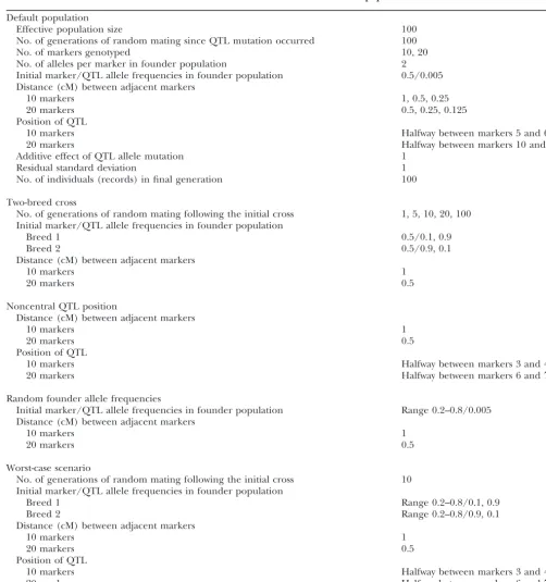
TABLE 2
Least-squares mean absolute difference (centimorgans) of QTL position estimates for four mapping methods using
10 or 20 markers under the default scenario
Method
SL SL2 HAP: IBD:
Marker spacing (cM) 10a 20 10 20 10 10
1 (0.5)b 1.48(*)c 1.14(**) 1.57(***) 1.58(***) 1.35(†) 1.36(†)
0.5 (0.25) 0.78(*) 0.63(**) 0.83(***) 0.81(†) 0.71(‡) 0.68(‡)
0.25 (0.125) 0.45(*, **) 0.38(***) 0.45(*) 0.44(**) 0.40(†) 0.40(***,†)
The mean absolute difference of the QTL position estimate from its true position for each mapping method (SL, regression on a single marker; SL2, regression on two markers; HAP, regression on a two-locus haplotype; IBD, likelihood based on haplotypes) used in populations created under the default scenario is shown. The QTL is located in the center of the haplotype.
aIndicates the number of markers genotyped and used in the model.
bDistances without parentheses are for methods with 10 markers, while those inside parentheses are for
methods with 20 markers.
cFor a given marker spacing, least-squares means with different symbols (*, **, ***, †, ‡, §) are significantly
different (P⬍0.05).
good. At this marker spacing, an average QTL position to evaluate the approaches with more equitable geno-typing costs, considering that the IBD method requires estimate could be expected to deviate from the true
QTL position by⬍2 markers or marker brackets from knowledge of haplotypes. The HAP method also re-quires knowledge of haplotypes, but it was allowed to the QTL. Additionally, average mapping resolution
in-creased proportionately as the marker spacing de- use 20 genotypes to determine if additional information could improve its mapping resolution and to provide a creased. The average LSMDs across methods using 10
markers were 0.74 and 0.42 cM for marker spacings of more complete comparison. The SL method using 20 markers (SL-20) was significantly better than all other 0.5 and 0.25 cM, respectively. In both cases, an average
QTL position estimate could be expected to deviate methods at positioning the QTL in its true location when markers were spaced either 0.5 or 0.25 cM apart from the true QTL position by⬍2 markers or marker
brackets. (Table 2). However, when markers were spaced 0.125
cM apart (0.25 cM for IBD), SL-20 was not significantly The bias of all four methods under the default
simula-tion was approximately zero. The mean QTL posisimula-tion better than IBD. With 20 markers, SL2 was significantly poorer than SL-20 and IBD at positioning the QTL. estimate for each regression method differed from the
true QTL position byⱕ⫾0.05 cM, regardless of marker This regression method, SL2, may perform consistently worse than SL because more degrees of freedom are spacing. The IBD method’s mean QTL position estimate
differed from the true QTL position by 0.1 cM when associated with the markers for this model (2 d.f.) as compared to the SL model (1 d.f.).
the marker spacing was 1 cM and differed byⵑ0.02 cM
when the markers were spaced 0.5 and 0.25 cM apart. Again, biases of the regression-based methods were small (⬍⫾0.04 cM) except for the SL2 method with 20 A bias of zero was expected because the QTL was
posi-tioned in the center of the marker haplotype. markers at 0.5 cM marker spacing. Its mean position estimate differed from the true position by⫺0.12 cM. Comparing LSMD across methods, the IBD method
was significantly better at estimating the position of the However, at smaller marker spacings, bias of the SL2 method was⬍ ⫺0.04 cM.
QTL than the SL method with 10 markers (SL-10) for
all three marker spacings (Table 2). The SL-10 method In general, LSMD of the SL method was smaller when 20 markers were used as compared to 10 for all marker was significantly better than the SL2 method with 10
markers (SL2-10) when the marker spacings were 1 and spacings (Table 2). Interestingly, in the case of SL2, LSMD changed very little when 20 markers were used 0.5 cM. Interestingly, fitting a two-locus haplotype in
regression (the HAP method) using 10 markers per- as compared to 10 for all marker spacings (Table 2). So the ability to utilize extra information from additional formed similar to the IBD method regardless of marker
spacing. markers appears to be dependent upon the method of
analysis. Next, with the exception of HAP the regression
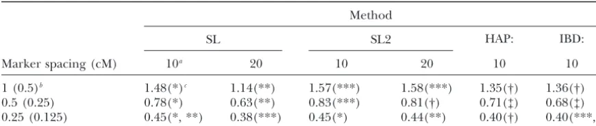
TABLE 3 from⫺0.17 to 0.16 cM. As the number of generations of random mating decreased, LSMD tended to increase.
Least-squares mean absolute difference (centimorgans) of
However, when the number of generations of random
QTL position estimate for mapping methods with 1-cM marker
mating decreased from 100 to 20, LSMD decreased for
spacing in a two-breed cross followed by random mating
all methods. This may be due to the fact that initially Method only two QTL alleles were in this population and after 100 generations of mating the QTL alleles attained ex-SL
treme frequencies or became fixed in many replicates,
Generations of IBD:
random mating 10a 20 10
resulting in lower mapping resolution.
In nearly all cases, the IBD method was significantly
100 2.34(*)b 2.1(**) 2.28(*)
better than the SL-10 method but not significantly
differ-20 2.27(*) 1.97(**) 2.01(**)
ent from the SL-20 method (Table 3). With 100
genera-10 2.35(*) 2.16(**) 2.08(**)
5 2.48(*) 2.28(**) 2.22(**) tions of random mating, however, the SL-20 method
1 2.51(*) 2.47(**) 2.40(**) was significantly better and there was no difference be-tween the IBD and SL-10 methods. When only one gen-The mean absolute difference of the QTL position estimate
eration of random mating occurred after the cross, a from its true position for each mapping method (SL,
regres-sion on a single marker; IBD, likelihood based on haplotypes) situation comparable to an F2population, the SL-20 and used in populations created under the crossbred scenario is IBD methods were better than the SL-10 method. A shown. The position of the QTL is the center of the haplotype, basic assumption of the IBD method was violated in this and the effective population size is 100.
population,i.e., the event that created linkage disequi-aIndicates the number of markers genotyped and used in
librium. It was expected that the mapping accuracy of the model.
bFor a given number of generations, least-squares means the IBD method would be more negatively affected than
with different symbols (*, **) are significantly different (P⬍ the mapping accuracy of regression methods because
0.05). they make no assumptions about population history.
However, both methods had similar mapping accura-cies. So, violating this assumption had no impact on the comparison of the methods.
had the same two QTL alleles but at different
frequen-cies (see Table 1). The number of generations of ran- Noncentral QTL position: In this population, the QTL was positioned halfway between markers 3 and 4 dom mating that occurred after the initial cross of the
two breeds ranged between 100 and 1. The LSMDs for (or markers 6 and 7 when 20 markers were genotyped) and the IBD method was compared to the SL method the IBD method and the SL method with 10 (20)
mark-ers for each of the different numbmark-ers of generations of with 10 (20) markers. The LSMD for each method with marker spacing of 1 (0.5) cM is presented in Table 4. random mating are shown in Table 3. Marker spacing
was set to 1 (0.5) cM, and the QTL was located at the Both the SL-10 method and the IBD method had larger LSMDs when the QTL was positioned toward the center of the marker haplotype. Due to the poor
perfor-mance of the SL2 method in the default population, it beginning of the marker haplotype instead of at the center. However, the LSMD of the SL-20 method did was not tested in any of the alternative populations. The
HAP method was not tested in any of the alternative not change when the QTL was positioned toward the beginning of the marker haplotype. For this population, populations to focus on the comparison between
single-marker-based analysis and the IBD method. the SL-20 method was best able to estimate the position of the QTL while the SL-10 method was least able. How-Population admixture affected the accuracy of all
methods negatively (Table 3). Even with 100 genera- ever, all methods had much greater mapping accuracy than that of a randomly selected QTL position. The tions of random mating, LSMD was greater than that
in the default population for both methods (Table 2). LSMD for a randomly chosen QTL position is 2.4 cM when 10 markers (1-cM spacing) are used and the QTL In fact, the LSMD of the IBD and regression methods
was often greater than the LSMD of a randomly selected is between markers 3 and 4 and 2.58 cM when 20 mark-ers (0.5-cM spacing) are used and the QTL is located QTL position, which is 2 cM for the 10-marker case
(1 cM spacing) and 2.25 cM for the 20-marker case between markers 6 and 7.
Bias was observed in all methods, as expected, due (0.5 cM spacing) with a centrally located QTL. Note,
however, that a centrally located QTL is most favorable to the noncentral position of the QTL. Bias was smallest for the SL-20 method, at 0.36 cM, followed by the IBD for a random estimator of QTL position;i.e., the LSMD
of a randomly selected QTL position will be smallest method at 0.51 cM, and the SL-10 method at 0.63 cM (Table 4). Although bias of the SL-20 method increased when the true QTL is located in the center of the
chro-mosome. All of the simulated populations, except for from 0.02 to 0.36 cM with a noncentral position of the QTL, LSMD of the SL-20 method did not change (Ta-the noncentral QTL and worst-case scenario, included
a centrally located QTL. So, the accuracy of the methods ble 4). Unlike the SL-20 method, the SL-10 and IBD methods showed an increase in both bias and LSMD is compared to the most accurate random QTL position
TABLE 4
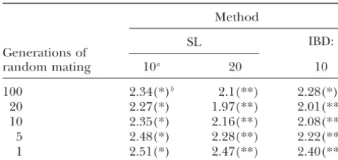
Least-squares mean absolute difference (centimorgans) of QTL position estimate and bias (centimorgans) for mapping methods in three alternate scenarios
Method
SL
Marker spacing IBD:
Alternate scenario (cM) 10a 20 10
Noncentral QTL position 1 (0.5)b LSMD 1.54(*)c 1.14(**) 1.38(***)
Bias 0.63 0.36 0.51
Random founder allele frequencies 1 (0.5) LSMD 1.44(*) 1.18(**) 1.36(***)
Bias ⫺0.09 0.02 ⫺0.03
Worst-case scenario 1 (0.5) LSMD 2.67(*) 2.43(**) 2.45(**)
Bias 1.76 1.49 1.56
The mean absolute difference of the QTL position estimate from its true position and bias for each mapping method (SL, regression on a single marker; IBD, likelihood based on haplotypes) used in populations created under three alternate scenarios is shown.
aIndicates the number of markers genotyped and used in the model.
bDistances without parentheses are for IBD with 10 markers, while those inside parentheses are for models
with 20 markers.
cFor a given alternate scenario, least-squares means with different symbols (*, **, ***) are significantly
different (P⬍0.05).
remained relatively small though, as the bias for a ran- The IBD method and the SL method using 10 (20) markers were tested for this worst-case scenario with a domly selected QTL position is 2 cM for both the
10-and 20-marker case. marker spacing of 1 (0.5) cM and their LSMDs are
shown in Table 4. The LSMD of all methods increased
Variable marker allele frequencies: In all previous
populations, initial frequency of the marker alleles was drastically compared to the default population. The av-erage LSMD for the SL-10, SL-20, and IBD methods 0.5. Here marker allele frequencies in the founders were
randomly set at each marker locus within a range of 0.2 increased from 1.33 cM under the default conditions to 2.52 cM in this population. The LSMDs of the three and 0.8 and then the IBD method was compared to the
SL method using 10 (20) markers. The LSMDs for these methods were similar to the LSMD of a randomly se-lected QTL position, which is 2.4 cM when 10 markers methods at a marker spacing of 1 (0.5) cM are shown
in Table 4. (1-cM spacing) are used and 2.58 cM when 20 markers
(0.5-cM spacing) are used and the QTL is in a non-The performance of all methods in this population
was similar to their performance in the default popula- central location as mentioned previously. Biases also increased markedly, from a range of⫺0.04 to 0.1 cM tion (Tables 2 and 4). The LSMDs of all methods
in-creased by 0.04 cM or less from their LSMDs in the in the default scenario, to a range of 1.49 to 1.76 cM in the worst-case scenario (Table 4). These values are default. Additionally, the bias for all three methods
re-mained close to zero, ranging from 0.03 to⫺0.09 cM similar to the bias of a randomly selected QTL position, which is 2 cM as described previously. Bias was toward (Table 4). Comparing methods, the LSMD of the
SL-20 method was smallest, while the LSMD of the SL-10 the center of the chromosome for all methods. The large positive bias and the near doubling of the LSMD method was highest. This ranking of methods is the
same as for the default population. So, it appears that when compared to the default are unique to this popula-tion. However, when comparing LSMD across methods, the SL and IBD methods were not sensitive to marker
allele frequencies. the results are not unique. Here the SL-20 method was
not significantly different from the IBD method, and
Worst-case scenario:The previous alternative
popula-tions differed from the default by only one condition. both were significantly better than the SL-10 method. This result is similar to the results from the two-breed Here, several conditions were changed from the default
population to create a worst-case scenario. First, the two cross in which, in nearly all cases, the SL-20 method and the IBD method were similar and significantly bet-breeds described previously were crossed, followed by
ter than SL-10 (Table 3). 10 generations of random mating. Second, the QTL
was positioned between marker loci 3 and 4 when 10 markers were genotyped and between marker loci 6
DISCUSSION and 7 when 20 markers were genotyped. Third, marker
on a single marker is an effective method for LD-based by violations of these assumptions such as altering effec-fine mapping of QTL if a dense marker map is available. tive population size and the number of generations of In situations that were both ideal and nonideal for the random mating since the mutation occurred. However, IBD method ofMeuwissenandGoddard(2000), map- they did not consider an alternative event to create the ping precision of the IBD method was greater than that initial linkage disequilibrium.
of the SL method, given an equal number of markers. In two alternative populations in this study, the two-Mapping precision of the SL method using 20 markers breed cross and the worst-case scenario, a cross between was similar to or greater than that of the IBD method two breeds created initial disequilibrium. It may be that with 10 markers. It should be pointed out, however, these two breeds diverged from a common population that mapping precision of the SL method was underesti- several generations ago and were reintroduced.Sabry mated in the populations simulated here, because the et al. (2002) tested the IBD method in a population SL method estimates the position of the QTL at a similar to this in which four populations diverged from marker locus, but the true position of the QTL was a founder population, were reintroduced after 90 gener-always simulated at the center between two marker loci. ations, and were allowed to randomly mate for 6 genera-Thus, the most accurate QTL position estimate the SL tions.Sabryet al. (2002) found the IBD method to be method can have is at one of the markers flanking the robust to this population structure, in contrast to our true QTL, which introduces an inherent level of error result, which found that performance of the IBD method for the simulations performed here. In contrast, the was much worse in the two-breed cross and the worst-IBD method estimates the position of the QTL at the case scenario than in the default population. However, center of a marker bracket, which is where the QTL is the regression methods also performed much worse in simulated, so it does not have an inherent error. these two alternative populations than in the default The comparable performance of the IBD and SL population (Tables 2–4). In fact, the mapping accuracy methods is contradictory to the generally held expecta- of all methods was similar to, or even less than, the ac-tion that using more informaac-tion (i.e., a haplotype) curacy of a randomly selected QTL position for both results in better estimates. One possible explanation is alternative populations. The worst-case scenario does that IBD probability matrices were similar for adjoining include a noncentral QTL and randomly set marker positions of the QTL. In other words, IBD probability allele frequencies, which the two-breed cross does not, matrices were not sensitive to the position of the QTL.
but these were shown to have little effect on mapping Thus, for adjoining positions of the QTL the likelihoods
ability. So the decrease in mapping accuracy for all were also similar, possibly resulting in decreased
map-methods is apparently due to the introduction of popu-ping precision. Further studies will examine how the
lation admixture. Other population events such as re-number of markers considered in the haplotype affects
cent bottlenecks or recurrent mutation at the QTL may the sensitivity of the IBD probability matrices and
map-also decrease the ability of the methods to fine map a ping precision.
QTL. Further research is needed to compare methods Another possible explanation for this contradictory
under these scenarios. result may stem from the fact that the regression-based
Second, any or all methods may be affected if the methods model the disequilibrium using location
pa-QTL is not located in the center of the chromosomal rameters (mean effects of marker alleles), while the
region evaluated. If the QTL is closer to either end of IBD method models the disequilibrium using dispersion
a chromosomal region, then there will be fewer markers parameters (variance of genotypic values and error
vari-on vari-one side of the QTL than vari-on the other. Thus, there ance). It is well known that location parameters are
is no longer a symmetric distribution of information easier to estimate than dispersion parameters. Thus,
across the chromosomal region. The fact that LSMD of single-marker regression-based methods may have an
the SL-20 method did not change when the QTL posi-inherent advantage over the IBD method.
tion was shifted toward the beginning of the
chromo-Effects of alternative populations:Several alternative
some (Table 4) supports this idea. The SL-20 method populations were considered in this study to test
ro-maintained six markers to the left of the alternative bustness of the fine-mapping methods and to determine
QTL position while the IBD and SL-10 methods main-if any methods were particularly sensitive to deviations
tained only three markers. The additional marker infor-from the default population.
mation may have allowed the SL-20 method to map the First, in the default, it was assumed that a mutation
QTL equally well at both QTL positions. Also, additional on a founder chromosome was responsible for creating
marker information may have allowed the SL-20 method the linkage disequilibrium in the population. The IBD
to maintain smaller bias than the SL-10 or IBD method probabilities were generated under the assumption that
with a noncentral QTL (Table 4). The finite parameter 100 generations of random mating in a population of
space considered for the noncentral QTL introduced effective size 100 had elapsed since the mutation
oc-bias for all methods. Bias of SL-10 was largest (Table 4), curred.MeuwissenandGoddard(2000) showed that
decreased marker spacing, of SL-20 greatly improved of a QTL in livestock has appeared only recently (
Gri-sartet al. 2001;Blottet al. 2003). These studies showed
its mapping accuracy.
Third, IBD probabilities were calculated under the that fine mapping of a previously identified chromo-somal region was an important step toward identifica-assumption that initial frequencies of all marker alleles
were 0.5 and violating this assumption may have an tion of the gene and its causative mutation(s). Using a maximum-likelihood approach that simultaneously effect on the IBD method. A marker is most informative
when its frequency is 0.5 so marker allele frequencies mined linkage and LD information in outbred half-sib pedigrees from five different dairy cattle populations, that deviate from 0.5 should also affect any fine-mapping
method. However, results from this study showed that Farniret al. (2002) were able to refine the position of a previously identified QTL on BTA 14. This eventually the IBD method and the regression-based methods
per-form as well in this alternative population as in the led to the positional cloning of theDGAT1gene (
Gri-sart et al. 2001). Blott et al. (2003) modified the
default population. Thus, the deviation of marker
fre-quencies from 0.5 had essentially no impact on the method ofFarniret al. (2002) to consider IBD probabil-ities for sires’ haplotypes so that a hierarchical clustering ability of the methods to map the QTL. This is an
impor-tant result because it seems unlikely that in an actual algorithm could be used to group haplotypes to fine map a QTL on BTA 20 affecting milk yield and composi-population the frequencies of all marker alleles would
be 0.5. Markers with more extreme allele frequencies tion. The bovine growth hormone receptor gene (GHR) was identified as a positional candidate gene and muta-were not considered because they would not be utilized
in an experimental situation. So the range of founder tion inGHRwas found to be associated with milk yield and composition (Blottet al. 2003).Meuwissenet al. allele frequencies used in this population is reasonable
because it does not cause marker alleles to have extreme (2002) extended the IBD method of Meuwissen and Goddard(2000) to also include pedigree information frequencies or to reach fixation in generation 100 such
that mapping precision is decreased. Although all meth- and fine mapped a QTL for twinning rate in dairy cattle to a region ⬍1 cM. Each of these experiments took ods were robust to this alternative population, the SL-20
method was again best able to estimate the position of advantage of both linkage and LD information for the purposes of fine mapping, so results from this study the QTL and thus would be the preferred method for a
fine-mapping experiment if the markers were available. cannot be extrapolated directly to form a comparison between regression-based fine-mapping methods and
Estimation of IBD probabilities:As noted earlier, IBD
probabilities were not obtained for every possible hap- the fine-mapping methods used inGrisartet al. (2001), Meuwissen et al. (2002), orBlottet al. (2003). lotype pair but instead were estimated for groups of
haplotype pairs that shared a similar distribution of IIS However, it can be stated that if a fine-mapping exper-iment was to be conducted using a sample of individuals marker alleles around the QTL.Meuwissenand
God-dard (2000) presented the IBD probabilities derived assumed to be unrelated, regression-based LD mapping methods would be expected to perform as well as IBD-from the gene drop method as approximations to those
based on individual haplotype comparisons. In fact, the based LD mapping methods. If individuals were related, given the same number of individuals, the expected IBD probabilities based on haplotype pairs are identical
to IBD probabilities based on (Nl,Nr) categories. This number of informative markers and haplotypes would decrease, which could decrease mapping precision. is because the IBD state of two-QTL alleles is dependent
upon only the number of consecutive marker alleles MeuwissenandGoddard(2000) showed that mapping precision of their IBD method decreased when pheno-flanking the QTL that are IIS. The first pair of non-IIS
alleles that is reached indicates a recombination event typic records from 100 individuals in a population of effective size 50 were used as compared to records from in the population simulated here. Thus, marker alleles
beyond this locus are no longer informative for de- the default population of effective size 100. However, the decrease in mapping precision was not large ( Meu-termining the IBD state of the QTL alleles. This was
confirmed by simulating a default population with 4 wissenandGoddard2000). Further research is neces-sary to examine whether population size and relation markers instead of 10 and calculating an IBD probability
for each haplotype pair. The IBD probability of each between individuals will impact LD-based mapping methods.
haplotype pair was the same as the IBD probability of
the appropriate (Nl,Nr) category for the haplotype pair. Evidence to support our result that single-marker-based analysis is comparable to haplotype-single-marker-based analysis This is an important result because if IBD probabilities
are based on individual haplotype pairs, the number was presented in a recent study byZhanget al. (2003), where a variance-components analysis (Abecasis et al. of IBD probabilities that must be estimated increases
exponentially as the number of markers increases. The 2000) was used to detect association between markers and immunoglobulin E concentration in humans. The ability to group haplotype pairs into (Nl,Nr) categories
is essential for the efficient use of the IBD method. association results that were obtained using a three-, four-, or five-marker haplotype as a sliding window across
Current use of fine-mapping methodology:The
re-sults obtained using single markers (Zhanget al. 2003).
periment Station, and by Hatch Act and State of Iowa funds. Laura Future studies using experimental data rather than
sim-Grapes was supported by a United States Department of Agriculture ulated data should also examine haplotype- and single- National Needs fellowship in quantitative and molecular genetics. marker-based analyses to determine their mapping
pre-cision under experimental conditions.
Mapping under equitable resources:Justification for LITERATURE CITED
the use of 20 markers in regression analysis comes from Abecasis, G. R., L. R. CardonandW. O. C. Cookson, 2000 A gen-the need to compare methods as gen-they could be used in eral test of association for quantitative traits in nuclear families.
Am. J. Hum. Genet.66:279–292. an experimental situation. For the population described
Blott, S., J. Kim, S. Moisio, A. Schmidt-Ku¨ ntzel, A. Cornet et
here, resources required to conduct an experiment us- al., 2003 Molecular dissection of a quantitative trait locus: a ing information from a 10-locus haplotype are more phenylalanine-to-tyrosine substitution in the transmembrane domain of the bovine growth hormone receptor is associated comparable to resources required to conduct an
experi-with a major effect on milk yield and composition. Genetics163:
ment using information from 20-marker, rather than
10-253–256.
marker, genotypes. In practice, it is possible to estimate Bodmer, W. F., 1986 Human genetics: the molecular challenge. Cold Spring Harbor Symp. Quant. Biol.LI:1–13.
haplotype information without knowing parental
geno-Darvasi, A., and M. Soller, 1995 Advanced intercross lines, an types or to infer the haplotypes when half-sib family experimental population for fine genetic mapping. Genetics141: information is available, but the IBD method as pre- 1199–1207.
Farnir, F., B. Grisart, W. Coppieters, J. Riquet, P. Berziet al., sented by Meuwissen and Goddard (2000) requires
2002 Simultaneous mining of linkage and linkage disequilib-known haplotypes from equally unrelated individuals rium to fine map quantitative trait loci in outbred half-sib pedi-with no pedigree information. The effect of using esti- grees: revisiting the location of a quantitative trait locus with major effect on milk production on bovine chromosome 14. mated haplotype information in the IBD method has
Genetics161:275–287.
not been studied, but it is expected that this will reduce Grisart, B., W. Coppieters, F. Farnir, L. Karim, C. Fordet al., 2001 mapping accuracy. It is debatable whether it is statisti- Positional candidate cloning of a QTL in dairy cattle: identifica-tion of a missense mutaidentifica-tion in the bovineDGAT1gene with major cally fair to compare the SL-20 method to the IBD
effect on milk yield and composition. Genome Res.12:222–231. method with 10 markers but for experimental purposes Meuwissen, T. H. E., andM. E. Goddard, 2000 Fine mapping of quantitative trait loci using linkage disequilibria with closely described here it was considered fair.
linked markers. Genetics155:421–430. The benefit of using 20 instead of 10 markers was
Meuwissen, T. H. E., A. Karlsen, S. Lien, I. OlsakerandM. E. most evident in the default population (Table 2) and Goddard, 2002 Fine mapping of a quantitative trait locus for twinning rate using combined linkage and linkage disequilibrium in the following two alternative populations (Table 4):
mapping. Genetics161:373–379.
(1) for a noncentral QTL and (2) when marker allele Rabinowitz, D., 1997 A transmission disequilibrium test for quanti-frequencies were random. So genotyping additional tative trait loci. Hum. Hered.47:342–350.
Sabry, A., M. S.Lundand B.Guldbrandtsen, 2002 Robustness markers can improve the SL method’s ability to fine
of a variance component QTL fine mapping method. Proceed-map a QTL by making it more robust. Of course, de- ings of the 7th World Congress on Genetics Applied to Live-pending on the extent of the LD, there will be a limit stock Production, August 19–23, Montpellier, France, Vol. 32,
pp. 677–680. to the extra information that can be obtained by simply
Taylor, B. A., 1978 Recombinant inbred strains: use in gene map-genotyping additional markers. It may be possible that ping, pp. 423–438 inOrigins of Inbred Mice, edited by H. C.Morse. an optimum number of markers spaced an optimum Academic Press, New York.
Xiong, M., andS. Guo, 1997 Fine-scale mapping of quantitative trait distance apart exist for fine mapping. Further work is
loci using historical recombinations. Genetics145:1201–1218. being conducted to examine this theory and to examine Zhang, Y., N. I. Leaves, G. G. Anderson, C. P. Ponting, J. Brox-holmeet al., 2003 Positional cloning of a quantitative trait locus additional properties of haplotype-based LD mapping.
on chromosome 13q14 that influences immunoglobulin E levels The authors thank Dan Nettleton for his comments and contribu- and asthma. Nat. Genet.34:181–186.
tion to this work. This work was supported in part by funding from the