Combined Linkage and Association Mapping of Quantitative Trait Loci by Multiple Markers

(1)

©

DOI: 10.1534/genetics.104.035147

Combined Linkage and Association Mapping of Quantitative

Trait Loci by Multiple Markers

**Jeesun Jung,* Ruzong Fan**

†,1

_{and Lei Jin}

†

*Department of Human Genetics, University of Pittsburgh, Graduate School of Public Health, Pittsburgh, Pennsylvania 15261 and†_{Department of Statistics, Texas A&M University, College Station, Texas 77843}

Manuscript received August 18, 2004 Accepted for publication February 10, 2005

ABSTRACT

Using multiple diallelic markers, variance component models are proposed for high-resolution combined linkage and association mapping of quantitative trait loci (QTL) based on nuclear families. The objective is to build a model that may fully use marker information for fine association mapping of QTL in the presence of prior linkage. The measures of linkage disequilibrium and the genetic effects are incorporated in the mean coefficients and are decomposed into orthogonal additive and dominance effects. The linkage information is modeled in variance-covariance matrices. Hence, the proposed methods model both association and linkage in a unified model. On the basis of marker information, a multipoint interval mapping method is provided to estimate the proportion of allele sharing identical by descent (IBD) and the probability of sharing two alleles IBD at a putative QTL for a sib-pair. To test the association between the trait locus and the markers, both likelihood-ratio tests andF-tests can be constructed on the basis of the proposed models. In addition, analytical formulas of noncentrality parameter approximations of the

F-test statistics are provided. Type I error rates of the proposed test statistics are calculated to show their robustness. After comparing with the association between-family and association within-family (AbAw) approach by Abecasis and Fulkeret al., it is found that the method proposed in this article is more powerful and advantageous based on simulation study and power calculation. By power and sample size comparison, it is shown that models that use more markers may have higher power than models that use fewer markers. The multiple-marker analysis can be more advantageous and has higher power in fine mapping QTL. As an application, the Genetic Analysis Workshop 12 German asthma data are analyzed using the proposed methods.

I

N linkage disequilibrium (LD) mapping or associa- using two markers are proposed for high-resolution link-tion study, one may use one marker a time. However, age and association mapping of quantitative trait loci the resolution of the single-marker analysis strategy can (QTL) based on population and pedigree data (Zhao be low. In addition, utilizing different markers may lead et al.2001;Fan andXiong2002, 2003;Fan andJung to different results, since the power to detect allelic 2003;Fanet al.2005). The genetic effects are orthogo-association depends on specific properties of the mark- nally decomposed into summation of additive and domi-ers. This complicates the interpretation of an analysis. nance effects. InAbecasiset al.(2000a,b, 2001), Car-It is interesting and important to build models that don(2000),Fulkeret al.(1999), andShamet al.(2000), use multiple markers simultaneously for high-resolution an association between-family and association within-mapping of genetic traits. A unified analysis using multi- family (AbAw) approach is proposed to decompose the ple markers gives a unique result and may lead to greater _{genetic association into effects of between pairs and} resolution. Moreover, large numbers of single-nucleotide _{within pairs. The models of our previous work differ} polymorphisms (SNPs) are available, and high-throughout _{from the AbAw approach in the following senses: (1)} genotyping approaches are emerging (International _{The AbAw approach uses only one marker in analysis,} SNP Map Working Group 2001). This encouraging _{but we use two diallelic markers, and (2) the way of} development facilitates high-resolution fine mapping of _{modeling mean coefficients is different.}_Fan_and_Jung genetic traits. It is natural and necessary to develop high- _{(2003) compare our method with the AbAw approach} resolution multiple-marker-based methods to dissect ge- _{and find that our method is advantageous for sib-pair}

netic traits. _{data. In addition,} _Fan _{et al.} _{(2005) confirm that our}

In our previous work, variance component models _{approach is more powerful than the AbAw approach}

for large pedigrees. One may note that it is not clear how to extend the AbAw approach to use more than one

1_{Corresponding author:}_{Department of Statistics, Texas A&M}

Univer-marker in analysis (R. FanandG. R. Abecasis,personal sity, 447 Blocker Bldg., College Station, TX 77845.

E-mail: [email protected] communication).

(2)

This article extends our previous work and investi- column vector at thejth marker locusMj. Hereyfis the

trait value of the father, andGfjis the genotype of the gates variance component models in high-resolution

linkage and association mapping of QTL using multiple father at thejth marker. Likewise, the other notations of the mother and theith child are defined accordingly diallelic markers. The models jointly take linkage and

with subscriptsmandi, respectively. The superscript␶ linkage disequilibrium information into account. The

denotes the transpose of a vector or a matrix. Under linkage information is modeled in the

variance-covari-the assumption of multivariate normality, we consider ance matrix, and the linkage disequilibrium

informa-the mixed-effect model tion is modeled in mean coefficients of trait values such

as the AbAw approach. By modeling the linkage

infor-yi⫽ ␤ ⫹wi␥ ⫹

兺

k

j⫽1

xi j␣j ⫹

兺

k

j⫽1

zi j␦j⫹Bi ⫹ei (1)

mation in the variance-covariance matrix, we may take advantage of much research on variance component

models (HasemanandElston1972;Amoset al.1989; (Searleet al.1992;PinheiroandBates2000), where Goldgar and Oniki 1992; Amos 1994; Fulker et al. _␤is the overall mean of fixed effect,wiis a row vector 1995;AlmasyandBlangero1998;Georgeet al.1999; of covariates such as sex and age,␥ is a column vector Prattet al.2000). In the mean time, the linkage disequi- of fixed-effect regression coefficients of wi, Bi is the librium information is incorporated into the mean coef- familial effect of random effects, andeiis the error term. ficients via indicator variables of marker genotypes, whose Assume thateiis normalN(0,␴2e), andBiis normalN(0, validity can be justified intuitively (FanandXiong2002, ␴2

s⫹ ␴2Ga), where␴2eis error variance,␴2sis the variance

pp. 608–609). of shared environment effect, and ␴2

Ga is the variance

Using the models developed in this article, test statis- of additive polygenic effect. Moreover, Bi and ei are tics can be developed for high-resolution association independent. For j ⫽ 1, · · · , k, ␣j and ␦j are fixed-mapping of QTL. The procedure is to perform appro- effect regression coefficients of the dummy variablesxi j priate linkage analysis on the basis of a sparse genetic andzi j, respectively. Herexi j andzi j are indicator vari-map for prior linkage evidence. Then association study ables and are defined as follows:

can be carried out on the basis of a dense genetic map for high-resolution mapping of QTL in the presence of

xi j⫽ ⎧ ⎭ ⎫ ⎩

2Pm_j ifGi j⫽MjMj

Pm_j⫺PM_j ifGi j⫽Mjmj

⫺2PM_j ifGi j⫽mjmj (2) prior linkage information. Likelihood-ratio tests (LRT)

can be carried out in high-resolution association studies. For large-sample data, likelihood-ratio criteria are accu-rate. On the basis of general theory of linear models,

F-test statistics can be built to test the association be- zi j⫽ ⎧ ⎭ ⎫ ⎩

⫺P2

m_j ifGi j⫽ MjMj

Pm_jPM_j ifGi j⫽ Mjmj

⫺P2

M_j ifGi j⫽ mjmj. tween trait locus and markers in the presence of prior

linkage evidence (Graybill1976). The analytical

for-Following the traditional quantitative genetics, the vari-mulas for the noncentrality parameter approximations

ance-covariance matrix of model (1) is a (l⫹2)⫻(l⫹

are derived for the F-test statistics. The merits of the

2) square matrix and is given by proposed method are investigated by power and sample

size comparison. Using the simulation program LDSI-MUL kindly provided by G. R. Abecasis, simulation study is performed to explore the power and type I error rates

of the proposed test statistics. The proposed methods _{⌺ ⫽}

⎛ ⎜ ⎜ ⎜ ⎜ ⎜ ⎝

1 ␳s ␳0 ␳0 … ␳0 ␳s 1 ␳0 ␳0 … ␳0 ␳0 ␳0 1 ␳12 … ␳1l ␳0 ␳0 ␳21 1 … ␳2l

⯗ ⯗ ⯗ ⯗ … ⯗

␳0 ␳0 ␳l1 ␳l2 … 1 ⎞ ⎟ ⎟ ⎟ ⎟ ⎟ ⎠

␴2_,

are compared with the AbAw approach (Abecasiset al.

2000a). Moreover, the method is applied to analyze the Genetic Analysis Workshop (GAW) 12 German asthma data (Wjst et al.1999;Meyerset al.2001).

where ␴2 ⫽ ␴2

g ⫹ ␴2s ⫹ ␴2Ga ⫹ ␴2e. Here ␴2g is variance

explained by the putative QTLQ. The genetic variance ␴2

g⫽ ␴2ga⫹ ␴2gdis decomposed into additive and

domi-MODEL

nance components. ␳s ⫽ ␴2s/␴2 is the correlation

be-Assume that kdiallelic markers Mj, j ⫽ 1, · · · , k, _{tween the parents. Let}␴2_H⫽ ␴2_s⫹ ␴2_Ga_{/2 be the variance} are typed in a region of one chromosome. Suppose a _{of familial effects that include shared environment} vari-quantitative trait locusQis located in the region, which _ance_␴2

sand half of the additive polygenic variance.␳0⫽

has two alleles Q1 and Q2 with frequencies q1 and q2, (␴2_ga/2 ⫹ ␴2_H)/␴2 is correlation between parents and

respectively. For marker Mj, there are two alleles Mj children;␳i j⫽ ␳j i⫽(␲i j Q␴2_ga⫹ ⌬i j Q␴2_gd⫹ ␴2_H)/␴2is the with frequencyPM_jandmjwith frequencyPm_j, respectively. correlation between the ith child and the jth child, where␲i j Qis the proportion of alleles shared identical For a nuclear family oflchildren and two parents, let

(3)

alleles at the putative QTL Q shared by the ith child and thejth child are IBD (Cotterman1940;Prattet

al.2000;ZhuandElston2000;Lange2002). On the _V

D⫽ ⎛ ⎜ ⎜ ⎜ ⎝

P2 M1P

2 m1 D

2

M1M2 … D 2 M1Mk

D2

M1M2 P 2 M2P

2

m2 … D

2 M2Mk

⯗ ⯗ … ⯗

D2

M₁M_k D2M₂M_k … P2M_kP2m_k ⎞ ⎟ ⎟ ⎟ ⎠

. (4) basis of the above discussion, the log-likelihood function

of the mixed-effect model (1) is given by

Inappendix a, the coefficients of model (1) are derived L⫽ ⫺l⫹2

2 log(2␲)⫺

1

2log|⌺|⫺ 1

2(y⫺X␩)

␶_⌺⫺1₍_y⫺_X␩_),

as

(3) _⎛

⎜ ⎜ ⎝

␣1 ⯗ ␣k

⎞ ⎟ ⎟ ⎠⫽

V⫺1 A

⎛ ⎜ ⎜ ⎝

2DM₁Q ⯗

2DMkQ ⎞ ⎟ ⎟ ⎠␣Q

and

⎛ ⎜ ⎜ ⎝ ␦1

⯗ ␦k

⎞ ⎟ ⎟ ⎠⫽

V⫺1 D

⎛ ⎜ ⎜ ⎝

D2 M₁Q ⯗

D2 MkQ

⎞ ⎟ ⎟ ⎠␦Q

. (5) where␩ ⫽ (␤,␥␶,␣1, · · · ,␣k,␦1, · · · ,␦k)␶is a vector

of regression coefficients, and Xis the model matrix, accordingly.

Equations (5) show that the parameters of LD (i.e., One may wonder why we use model (1) to describe

DM_iQ and DM_iM_j) and gene effect (i.e., ␣Q and ␦Q) are the phenotypes. Here we provide an intuitive rationale.

Suppose that QTLQ coincides with one marker, e.g., contained in the mean coefficients. Model (1) simulta-marker M1, and trait allele Q1 coincides with marker neously takes care of the LD and the effects of the

alleleM1 and allele Q2coincides with allele m1. Let ␮i j putative trait locusQ. The gene substitution effect ␣Q

is contained only in␣i; and the dominance effect␦Qis be the effect of genotypeQiQj,i,j⫽1, 2. Denote

geno-contained only in␦i,i⫽ 1, · · · ,k. Therefore, model typic valuea⫽ ␮11⫺(␮11⫹ ␮22)/2 andd⫽ ␮12⫺(␮11⫹

(1) orthogonally decomposes genetic effect into sum-␮22)/2. The average effect of gene substitution is␣Q⫽

mation of additive and dominance effects.

a⫹(q2⫺q1)d,i.e., the difference between the average

Assume that all markers Mi and Mj are in linkage effects of the trait locus alleles, and dominance

devia-equilibrium (i.e.,DM_iM_j⫽0,i,j⫽1, · · · ,k,i⬆j). The tion is␦Q⫽2din view of traditional quantitative genetics

(FalconerandMackay1996).FanandXiong(2002) coefficients of additive and dominance effects are given by␣1⫽(DM1Q/PM1Pm1)␣Q, · · · ,␣k⫽ (DMkQ/PMkPmk)␣Q,

show thatyican be expressed asyi⫽ ␮0⫹xi1␣Q⫹zi1␦Q⫹

Bi ⫹ ei, where ␮0 is overall population mean of the and ␦1 ⫽ (D2M₁Q/P2M₁P2m₁)␦Q, · · · , ␦k ⫽ (D2M_kQ/ quantitative trait. Hence, markerM1may fully describe P2MkP

2

mk)␦Q. That means markersM1, · · · ,Mk

indepen-the trait values if it coincides with indepen-the QTLQ. In practice, dently contribute to the analysis of the trait values. Usu-the information of QTLQis unknown. Instead, model ally, the markersMican be in LD, especially when they (1) is proposed to describe trait valueyiusing marker are located in a narrow chromosome region. Equations information. Two marker models were used in previous (5) correctly use the LD information of markersMi in work (FanandXiong2002, 2003;FanandJung2003; the analysis.

Linkage analysis can be performed by considering a

Fanet al.2005). Model (1) uses multiple markers and

reduced variance component model, is a natural generalization of model of our previous

work. The objective is to use marker information fully for

yi⫽ ␤ ⫹wi␥ ⫹Bi⫹ei, (6) fine high-resolution mapping of QTL. In the following,

by using the traditional method of variance component we show that model (1) and log-likelihood (3) can be

models (Amos et al. 1989; Amos 1994; Almasy and used in joint linkage and association mapping of QTL.

Blangero 1998). This initial study can identify prior linkage evidence of the trait values to a specific chromo-some region on the basis of a sparse genetic map.

Sup-PROPERTY OF REGRESSION COEFFICIENTS

pose that prior linkage evidence is provided by an initial

AND ASSOCIATION TESTS

linkage study. On the basis of a dense genetic map, Denote the measure of LD between trait locusQand _{high-resolution association mapping of the QTL can be} markerMi byDM_iQ⫽ P(MiQ1)⫺ PM_iq1, i⫽ 1, · · · , k carried out by fitting the full model (1). First, assume

that linkage is confirmed in a chromosome region by and the measure of LD between markerMiand marker

MjbyDM_iM_j⫽P(MiMj)⫺PM_iPM_j,i⬍j,i,j⫽1, · · · ,k. the significant presence of both the gene substitution and dominance effects, i.e., ␣Q ⬆ 0 and ␦Q ⬆ 0. On Let the additive and dominance variance-covariance

ma-the basis of Equations 5, ma-the existence of LD between trices of the indicator variables defined in (2) be (

appen-markersMi (i ⫽ 1, · · · , k) and trait locus Q can be dix a)

tested by Had: ␣1 ⫽ · · · ⫽ ␣k ⫽ ␦1 ⫽ · · · ⫽ ␦k ⫽ 0.

Second, assume that linkage is supported by the signifi-cant presence of the gene substitution effect, but not the dominance effect, i.e., ␣Q ⬆ 0 and ␦Q ⫽ 0. The

VA⫽2

⎛ ⎜ ⎜ ⎜ ⎝

PM1Pm1 DM1M2 … DM1Mk

DM₁M₂ PM₂Pm₂ … DM₂M_k

⯗ ⯗ … ⯗

DM₁M_k DM₂M_k … PM_kPm_k

⎞ ⎟ ⎟ ⎟ ⎟ ⎠

,

existence of LD can be tested by Ha:␣1⫽· · ·⫽ ␣k⫽

(4)

signifi-cant presence of the dominance effect, but not the gene where ␲i j M_lis the proportion of alleles shared IBD at substitution effect,i.e.,␣Q⫽0 and␦Q⬆0. The existence _{the marker}_M_l_for _l_⫽ _{1, · · · ,} _k_{. The coefficients} _␣_␲_, of LD can be tested by Hd:␦1⫽· · ·⫽ ␦k⫽0. ␤_␲M₁, · · · ,␤␲M_kare derived inappendix bas follows:

Evidence of association can be evaluated by the LRT procedure. For instance, let Lad be the log-likelihood

under the alternative hypothesis of Hadand L0 be the

⎛ ⎜ ⎜ ⎜ ⎝

␤␲M1

␤␲M2

⯗

␤␲Mk

⎞ ⎟ ⎟ ⎟ ⎠ ⫽ ⎛ ⎜ ⎜ ⎜ ⎝

1 (1⫺2␪M1M2)

2 _… ₍₁_⫺₂_␪ M1Mk)

2

(1⫺2␪M1M2)

2 ₁ _… ₍₁_⫺₂_␪

M2Mk)

2

⯗ ⯗ ⯗ ⯗

(1⫺2␪M1Mk)

2 ₍₁_⫺₂_␪ M2Mk)

2 _… ₁

⎞ ⎟ ⎟ ⎟ ⎠ ⫺1

log-likelihood under the null hypothesis Had. Then, the

likelihood-ratio test statistic 2[Lad⫺L0] is asymptotically

distributed as␹2_{. The degrees of freedom for this test}

are determined as follows. Under the null hypothesis

Had, there are onlykmeasures of LD,DM₁Q, · · · ,DM_kQ, ⫻

⎛ ⎜ ⎜ ⎜ ⎝

(1⫺2␪M1Q)

2

(1⫺2␪M2Q)

2

⯗

(1⫺2␪MkQ)

2 ⎞ ⎟ ⎟ ⎟ ⎠ . of which onlyk⫺1 are independent since兺k

i⫽1DM_iQ⫽0. Thus, the number of coefficients ␣i,␦i,i⫽1, · · · ,k,

And␣␲is estimated as␣␲⫽1⫺ ␤␲M1 ⫺ ␤␲M2 ⫺· · ·⫺

which is significantly different from 0, should beⱕk⫺

1 in a data analysis. This number is the degrees of free- ␤␲Mk. If markerMlcoincides with QTLQ, it can be shown

dom of the likelihood-ratio test statistic 2[Lad ⫺ L0]. that ␤_␲Ml⫽1 and ␣␲ ⫽ 0, ␤␲Mi⫽0,i⬆l. Hence

The likelihood-ratio test is accurate and robust for large _␲_ˆ_{i j Q}_{⫽ ␲i j M}

l. To estimate⌬i j Qof the probability of sharing

sample data based on the statistical theory. _{two alleles IBD for a sib-pair, consider} Theoretically, it is not easy to evaluate the power of

⌬ˆ_{i j Q}_⫽_E₍_⌬_{i j Q}_|_I_M

1,IM2, · · · , IMk)

the likelihood-ratio test statistics. The reason is that it

is very hard to calculate the approximations of non- _{⫽ ␣ ⫹ ␤}

M1␲i j M1⫹· · ·⫹ ␤Mk␲i j Mk⫹rM1⌬i j M1⫹· · ·⫹rMk⌬i j Mk,

centrality parameters of the likelihood-ratio test

statis-(8) tics.Shamet al.(2000) performed power analysis of the

AbAw approach by deriving the approximations of the where⌬i j M_lis the probability of sharing two alleles IBD noncentrality parameters of the likelihood-ratio test sta- _{at marker} _M_l _for _l _⫽ _{1, · · · ,} _k_{. The coefficients} tistics, which is rather complicated in our opinion. In ₍_r_M

1, · · · ,rMk)

␶_{are derived in}_{appendix c}_{as follows:} addition to the likelihood-ratio test statistics, we develop

an F-test procedure based on linear model theory in this article (Graybill1976). Utilizing the formulas of

⎛ ⎜ ⎜ ⎜ ⎝

rM1 rM2

⯗ rMk

⎞ ⎟ ⎟ ⎟ ⎠ ⫽ ⎛ ⎜ ⎜ ⎜ ⎝

1 (1⫺2␪M1M2)

4 _… ₍₁⫺₂␪ M1Mk)

4

(1⫺2␪M1M2)

4 ₁ _… ₍₁⫺₂␪

M2Mk)

4

⯗ ⯗ ⯗ ⯗

(1⫺2␪M1Mk)

4 ₍₁_⫺₂_␪ M2Mk)

4 _… ₁

⎞ ⎟ ⎟ ⎟ ⎠ ⫺1

noncentrality parameters in chapter 6 of Graybill (1976), the approximations of the noncentrality param-eters of theF-tests are calculated readily. Moreover, we show that the type I error rates and power of theF-test are

⫻ ⎛ ⎜ ⎜ ⎜ ⎝

(1⫺2␪M1Q)

4

(1⫺2␪M2Q)

4

⯗

(1⫺2␪MkQ)

4 ⎞ ⎟ ⎟ ⎟ ⎠ . very close to those of the likelihood-ratio test statistics

(Tables 2 and 3), which are actually guaranteed by the construction of theF-test for large samples (Graybill

The remaining coefficients are given inappendix cby 1976, pp. 187–188). Therefore, both the likelihood-ratio

test procedure and theF-test procedure are useful. Be-fore introducing the F-test procedure, we discuss the

⎛ ⎜ ⎜ ⎜ ⎝ ␤M1 ␤M2 ⯗ ␤Mk ⎞ ⎟ ⎟ ⎟ ⎠ ⫽ ⎛ ⎜ ⎜ ⎜ ⎝

␤␲M₁ ␤␲M₂ ⯗ ␤␲M_k

⎞ ⎟ ⎟ ⎟ ⎠ ⫺ ⎛ ⎜ ⎜ ⎜ ⎝

rM₁

rM₂ ⯗

rM_k ⎞ ⎟ ⎟ ⎟ ⎠ . parameter estimations first.

PARAMETER ESTIMATIONS The ␣ in Equation 8 is ␣ ⫽ 1⫺ ␤M₁ ⫺· · ·⫺ ␤M_k⫺

rM₁⫺ · · ·⫺rM_k. Again, if markerMlcoincides with QTL IBD estimations:Denote the recombination fraction

Q, it can be shown that⌬ˆi j Q⫽ ⌬i j M_l. between the trait locusQand markerMiby␪M_iQ,i⫽1,

Estimations of model coefficients and

variance-covar-· variance-covar-· variance-covar-· , k. Likewise, the recombination fraction between

iance matrix:As an example, assume that the data are markersMiandMjis defined by␪M_iM_j. FollowingFulker

composed of three subsamples:nindividuals of a

popu-et al. (1995) and Almasy and Blangero (1998), we

lation;mtrio families, each having both parents and a propose a multipoint interval mapping method to

esti-single child; and s nuclear families, each having both mate the proportion␲i j Qof allele sharing IBD at a

puta-parents and two offspring. Furthermore, we assume that tive QTLQfor a sib-pairiandjby

n, m, and sare sufficiently large, so that large sample theory applies. We may include data of nuclear families ␲ˆi j Q⫽E(␲i j Q|IM1,IM2, · · · ,IMk)

with both parents and more than two offspring. The ⫽ ␣␲⫹ ␤␲M1␲i j M1⫹ ␤␲M2␲i j M2⫹· · ·⫹ ␤␲Mk␲i j Mk, principle of the following paragraphs can be extended

(5)

to apply the large sample theory. To estimate the

param-F⫽ (H␩ˆ)

␶_[_H₍_X␶_⌺ˆ⫺1_X₎⫺1_H␶_]⫺1₍_H␩_ˆ)

y␶(⌺ˆ⫺1⫺ ⌺ˆ⫺1_X₍_X␶⌺ˆ⫺1_X₎⫺1_X␶⌺ˆ⫺1₎_y

(N⫺ 2k⫺1)

q

eters, one may take the method of interval mapping proposed by Fulker et al. (1995) and Almasy and

with a noncentralF(q, N ⫺ (2k ⫹ 1), ␭) distribution Blangero (1998). That is to say, for each location of

under the alternative hypothesis, where ␭ is the non-the QTL on non-the chromosome with fixed recombination

centrality parameter given by␭ ⫽(H␩)␶[H(X␶⌺⫺1_X₎⫺1

fractions, the IBD estimations are performed first. Then

H␶]⫺1₍_H␩_).

one may estimate parameters of⌺and␩as follows.

Combined analysis of population and family data:

Consider the overall log-likelihood L⫽兺I

i⫽1Li, I⫽

Again, assume that the data are composed of three

sub-n⫹m⫹s, whereLiis the log-likelihood of trait vector

samples:n individuals of a population;mtrio families, or valueyiof theith family or individual. Let⌺ibe the

each having both parents and a single child; ands nu-variance-covariance matrix of trait vector or valueyiand

clear families, each having both parents and two

off-Xibe its model matrix. Denote the total trait values by

spring. To calculate the approximations of the

non-y⫽(y␶1, · · · ,y␶I)␶, the total variance-covariance matrix

centrality parameters, assume that the sample sizesn, by⌺ ⫽diag(⌺1, · · · ,⌺I), and the model matrix byX⫽

m, andsare large enough that the large-sample theory (X␶1, · · · ,X␶I)␶. LetN⫽n⫹3m⫹4sbe the total number

applies. We show in appendix d the approximation of individuals. On the basis of the log-likelihood L⫽

兺I

i⫽1Li, parameters of ⌺ and ␩ can be estimated by

X␶⌺⫺1_X⫽

兺

n⫹m⫹s

i⫽1

X␶i⌺⫺i 1Xi⬇ diag(a1,a2VA,a3VD)/␴2, Newton-Raphson or Fisher scoring algorithms (

Jenn-richandSchluchter1986). Let ⌺ˆ ⫽ diag(⌺ˆ1, · · · , ₍₉₎

⌺ˆ_I_{) be the maximum-likelihood estimates of} _⌺_{. Then}

where a1, a2, and a3 are constants given by Equations

the estimate of␩is

(D7) inappendix d.

␩ˆ ⫽[X␶⌺ˆ⫺1_X_]⫺1_X␶_⌺ˆ⫺1_y_⫽_[_兺I

i⫽1X␶i⌺ˆi⫺1Xi]⫺1兺Ii⫽1X␶i⌺ˆ⫺i 1yi. _{The additive variance} ␴2

ga⫽ 2q1q2␣2Q and the domi-nance variance␴2

gd⫽(q1q2)2␦2Q are expressed in terms For each location of the QTL on the chromosome,

of the average effect of gene substitution ␣Q and the the likelihood-ratio test orF-test statistics can then be

dominance deviation␦Q. LetIkandI2kbekand 2k dimen-calculated using the estimates ⌺ˆ and ␩ˆ. The location

sion identity matrices. Moreover, letOk⫻lbe ak⫻lzero that gives the best result can be treated as the location

matrix. To test hypothesis Ha:␣1⫽ · · ·⫽ ␣k⫽ 0, the

of the QTL. In practice, some of the parameters (e.g.,

test matrixH⫽(Ok⫻1, Ik,Ok⫻k). Let us denote the test the variance parameter␴2

gd) may not be estimable and

statistic asFk,a. The noncentrality parameter is

approxi-identifiable due to the redundancy. For specific types

mated by of data, one needs to specify the model carefully.

␭k,a⬇

a2

␴2(␣1, · · · ,␣k)VA

⎛ ⎜ ⎜ ⎝ ␣1 ⯗ ␣k ⎞ ⎟ ⎟ ⎠

⫽4a2

␴2␣

2

Q(DM1Q, · · · ,DMkQ)V

⫺1 A ⎛ ⎜ ⎜ ⎝

DM1Q

⯗ DMkQ

⎞ ⎟ ⎟ ⎠

F-TESTS AND NONCENTRALITY PARAMETER

APPROXIMATIONS

On the basis of linear regression model theory, one

may constructF-test statistics of genetic effects and LD ⫽ a2␴2ga

␴2_q

1q2

(DM1Q, · · · ,DMkQ)(VA/2)

⫺1

⎛ ⎜ ⎜ ⎝

DM1Q

⯗ DMkQ

⎞ ⎟ ⎟ ⎠

. coefficients (Graybill 1976). Moreover, the

non-centrality parameters of theF-test statistics can be

calcu-To test hypothesis Hd:␦1⫽· · ·⫽ ␦k⫽0, the test matrix

lated readily. To evaluate the power of theF-test

statis-H⫽ (Ok⫻1, Ok⫻k, Ik). Let us denote the test statistic as tics, it is necessary to calculate the approximations of the

Fk,d. The noncentrality parameter is approximated by

noncentrality parameters. The procedure is as follows. First, one may construct anF-test statistic for each of

three hypotheses: ␭k,d⬇

a3

␴2(␦1, · · · ,␦k)VD

⎛ ⎜ ⎜ ⎝ ␦1 ⯗ ␦k ⎞ ⎟ ⎟ ⎠⫽ a3

␴2␦

2

Q(D2M1Q, · · · ,D

2 MkQ)V

⫺1 D ⎛ ⎜ ⎜ ⎝ D2 M1Q

⯗ D2

MkQ

⎞ ⎟ ⎟ ⎠

Had:␣1⫽· · · ⫽ ␣k⫽ ␦1 ⫽· · ·⫽ ␦k⫽ 0;

Ha:␣1⫽ · · ·⫽ ␣k⫽0;

Hd:␦1 ⫽· · ·⫽ ␦k⫽ 0. ⫽ a3␴

2 gd

␴2_q2

1q22

(D2

M1Q, · · · ,D

2 MkQ)V

⫺1 D ⎛ ⎜ ⎜ ⎝ D2 M1Q

⯗ D2

MkQ

⎞ ⎟ ⎟ ⎠

.

The noncentrality parameter of each F-test statistic

can be calculated using the theory inGraybill(1976, To test hypothesis Had: ␣1 ⫽ · · · ⫽ ␣k⫽ ␦1 ⫽ · · · ⫽ ␦k⫽ 0, the test matrixH⫽ (O2k⫻1,I2k). Let us denote Chap. 6). Assume that there are no covariates. Then

the coefficients of model (1) can be written as␩ ⫽(␤, the test statistic asFk,ad. The noncentrality parameter is ␭k,ad⬇␭a⫹ ␭d;i.e.,␭k,adis decomposed into the summa-␣1, · · · ,␣k,␦1, · · · ,␦k)␶. For each hypothesis, there is

aq⫻(2k⫹1) matrixH, such that the hypothesis can tion of additive and dominant noncentrality parameters.

Nuclear family data:To make a comparison with the be written as H␩ ⫽ 0, where q is the rank of H. On

the basis of Graybill (1976), the F-test statistic for results ofAbecasiset al.(2000a, Table 4), we consider

(6)

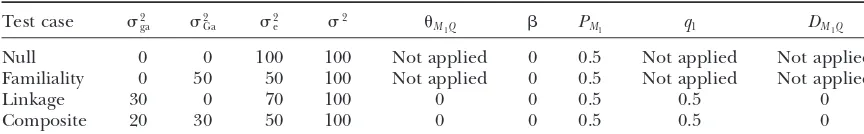
TABLE 1

The parameters of the simulated genetic cases

Test case ␴2

ga ␴2Ga ␴2e ␴2 ␪M1Q ␤ PM1 q1 DM1Q

Null 0 0 100 100 Not applied 0 0.5 Not applied Not applied

Familiality 0 50 50 100 Not applied 0 0.5 Not applied Not applied

Linkage 30 0 70 100 0 0 0.5 0.5 0

Composite 20 30 50 100 0 0 0.5 0.5 0

The total variance is fixed at ␴2⫽ ␴2

ga⫹ ␴2Ga⫹ ␴2e⫽100 and ␴2gd⫽ ␴2s⫽0. Admixture: no major gene

effect or familial effect␴2

g⫽ ␴2H⫽0, but with population admixture (see text for explanation).

N ⫽ I(l⫹ 2) be the total number of individuals. The mean of subpopulation A is fixed at 10 and the variance is fixed at 100, and the marker allele frequency PM₁ is other notations are defined in a similar way as above.

Suppose that variance-covariance matrices of theIfami- _{taken as 0.7 in subpopulation A. The trait mean of} lies are the same, i.e., ⌺1 ⫽ · · · ⫽ ⌺I. Denote⌺⫺i 1 ⫽ subpopulation B is fixed at 0 and the variance is fixed (1/␴2₎₍_{␥h j}₎

(l⫹2)⫻(l⫹2). If the sample size N is large at 100, and the marker allele frequencyPM₁ is taken as enough, we show inappendix e that _{0.3 in subpopulation B. Therefore, the total variance}

in the mixing population is␴2 ⫽ _{125. The admixture}

X␶⌺⫺1_X/I ⫽

兺

I

i⫽1

X␶i⌺⫺i 1Xi/I⬇diag(

兺

h,j

␥h j,b1VA,b2VD)/␴2,

contributed to (10⫺0)2_/[4⫻_125]⫽_{0.20 of the total}

variance. (10)

To calculate the type I error rates, 1000 data sets are where b1 andb2are constants given by Equations (E1) _{simulated for each test case. Each data set contains a}

inappendix e. The approximation of the noncentrality

certain number of related pedigrees. For instance, 120 parameter of statisticFk,ais _{trio families are generated for test case}

Nullif the total number of offspring is 120 and the number of offspring in each family is 1; but only 15 families are generated ␭k,a⬇

b1I␴2ga ␴2_q

1q2

(DM1Q, · · · ,DMkQ)(VA/2)

⫺1 ⎛ ⎜ ⎜ ⎝

DM1Q ⯗

DMkQ ⎞ ⎟ ⎟ ⎠

.

if the number of offspring in each family is 8 and the total number of offspring is 120. Using the data sets, we fit the model

TYPE I ERROR RATES _y_i_{⫽ ␤ ⫹}_x_i₁_␣₁ _⫹_B_i_⫹_e_i_,

To evaluate the type I error rates of the proposed _where _B

i is normalN(0,␴2Ga),yiis normalN(␤ ⫹ xi1␣1,

method, simulation program LDSIMUL kindly pro- _␴2_{), and} _␴2 _{⫽ ␴}2

ga⫹ ␴2Ga⫹ ␴2e. The null hypothesis is

vided by G. R. Abecasis is used to generate data sets. _H

1,a:␣1⫽0. Since the QTLQis in linkage equilibrium

Nuclear families are generated in simulation. Five test _{with marker}_M

1, an empirical test statistic that is larger

cases are considered in type I error rate calculation, _{than the cutting point at a 0.05 significance level is} which are taken fromAbecasiset al.(2000a, Table 2). _{treated as a false positive. On the basis of either the} Table 1 presents parameters of four test cases. Trait _{likelihood-ratio test or the}_F_{-test, type I error rates are} values are constructed by a normal distribution with _{calculated as the proportions of the 1000 simulation} mean 0 and total variance␴2_⫽_{100 except for test case}

data sets that give a significant result at the 0.05

signifi-ofAdmixture. Here␴2_{⫽ ␴}2

ga⫹ ␴2Ga⫹ ␴2eis the summation _{cance level based on} _F

1,a and the likelihood-ratio test

of the additive major gene effect ␴2

ga, the variance of _{statistic, respectively. Table 2 presents type I error rates}

polygenic effect␴2

Ga, and the error variance␴2e. In each _{of likelihood-ratio tests and}_F_{-test statistics. The results}

model except the Admixture, a diallelic marker M1 is _{show that the type I error rates are around the 0.05}

simulated with allele frequency PM1⫽0.5. In the test _{nominal significance level in almost all cases. Hence,}

cases ofNull,Familiality, andAdmixture, no major gene _{the proposed model is robust. In addition, the type I} effect is assumed,i.e.,␴2

ga⫽0. In the test cases ofLinkage _{error rates of} _F_{-tests are similar to those of the}

likeli-andComposite, major gene effect is assumed, and marker _{hood-ratio tests. In an association study, false positives}

M1coincides with the QTLQ,i.e., recombination frac- _{due to population stratifications are usually a big issue.}

tion ␪M₁Q⫽ 0; in the meantime, linkage equilibrium _{From the results of Table 2, the type I error rates in} is assumed between QTL Q and the marker M1, i.e., theAdmixture case are reasonable.

DM₁Q⫽ 0. In the test case ofAdmixture, population ad- Table 2, bottom, shows a notable variability in the range of type I errors when the number of offspring is mixture is generated by mixing families equally drawn

8 and the sample sizes are small. For example, the type from one of two subpopulations A and B. In both

sub-I error rates of theF-testFˆ1,a are 6.7% for test case of

populations A and B, no major gene effect or familial effect is assumed,i.e.,␴2

(7)

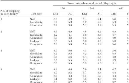
TABLE 2

Type I error rates (%) of test cases of Table 1 at a 0.05 significance level

Error rates when total no. of offspring is

120 240 480

No. of offspring

in each family Test case LRT Fˆ1,a LRT Fˆ1,a LRT Fˆ1,a

1 Null 5.0 4.9 5.1 5.1 5.8 5.8

Familiality 5.4 5.3 5.2 5.2 5.3 5.3

Admixture 3.9 3.8 5.2 5.2 5.3 5.3

2 Null 4.6 4.5 4.8 4.7 4.5 4.5

Familiality 4.2 4.1 3.6 3.6 4.7 4.8

Admixture 5.0 4.8 5.5 5.5 4.9 5.1

Linkage 5.5 5.4 5.0 4.3 5.0 5.1

Composite 5.6 5.8 5.8 5.9 5.6 5.7

4 Null 4.9 5.0 4.3 4.3 3.6 3.6

Familiality 5.2 5.3 4.2 4.3 4.8 4.8

Admixture 5.5 5.6 5.4 5.8 4.2 4.2

Linkage 5.3 5.5 5.4 5.4 4.9 5.0

Composite 5.3 5.5 5.3 5.3 4.1 4.2

8 Null 4.2 4.4 5.0 5.1 4.7 4.7

Familiality 4.7 5.3 5.1 5.5 4.4 4.4

Admixture 3.5 4.4 5.5 6.0 4.4 4.6

Linkage 6.1 6.8 4.3 4.6 4.6 4.8

Composite 5.8 6.7 5.5 5.9 3.7 3.9

The parameters are the same as those ofAbecasiset al.(2000a, Table 2).

This is most likely due to the small sample size and addition, D⬘ ⫽ DM₁Q/Dmax and Dmax⫽ min(PM₁,q1)⫺

multivariate normality. When the total number of off- _P_M

1q1. In the AbAw columns in Table 3, the results are

spring is 120, there are only 15 pedigrees, each con- _{taken from}_Abecasis_{et al.}_{(2000a, Table 4). In the (}_F

1,a,

sisting of two parents and 8 offspring; and the variance- _Fˆ

1,a, LRT)␶columns, the power (%) ofF1,ais calculated

covariance matrix ⌺ is a big 10 ⫻ 10 square matrix. _{on the basis of approximation of noncentrality} parame-Hence, the parameter estimations are hardly accurate, _ter_␭

1,a of test statistic F1,a at a 0.001 significance level;

which makes the deviation from the nominal level _{the power (%) of}_Fˆ

1,aand the LRT are calculated as the

greater. When the sample size increases (i.e., the total _{proportions of 1000 or 20,000 simulation data sets that} number of offspring is 240 or 480), the type I error _{give a significant result at the 0.001 significance level} rates are close to the nominal level of 0.05. The results _{based on}_F

1,aand the likelihood-ratio test statistic,

respec-of Table 2 are based on 1000 simulated data sets, which _{tively. For each simulated data set, a certain number} may not be always reliable. To further investigate the _{nuclear families are simulated via LDSIMUL. For} in-issue, we perform a calculation in the next section based _{stance, for one sib per family, 480 trio families are} simu-on 20,000 simulated data sets for anotherCompositetest _{lated in each simulated data set.}

case in Table 3. The results of Table 3 confirm that the _{The results of Table 3 clearly show that the proposed} type I error rates are close to the nominal level for large- _F_-tests_F

1,aand likelihood-ratio tests are much more

pow-sample data. _{erful than the AbAw approach. When}_D_{⬘ ⫽}_D

M₁Q/Dmaxⱖ

25%, it is possible to achieve considerable power. When

D⬘ ⫽DM₁Q/Dmaxⱖ 50%, the statisticF1,ais powerful for

POWER CALCULATION AND COMPARISON

a sample with a total number of 480 sibs. In addition,

Comparison with the AbAw approach: Denote the _{the results of Table 3 show that the empirical power of} heritability byh2_{, which is defined as}_h2⫽ ␴2

ga/␴2(Fal- _Fˆ_1,a _{is similar to that of the likelihood-ratio test. This} coner and Mackay 1996). To compare the method _{implies that in a large sample the two tests provide} proposed in this article with the AbAw approach of _{similar power (}_Graybill _{1976). The AbAw approach} Abecasiset al.(2000a), we present a power comparison _{presented in}_Abecasis _{et al.} _{(2000a) utilized only the} in Table 3. The parameters are the same as those of _{trait values of sibships in the model and discarded the} Abecasis et al.(2000a, Table 4): q1 ⫽PM₁⫽ 0.5, h2⫽ trait values of parents. This is, obviously, not an efficient way. The proposed methods, on the other hand, incor-0.1,␴2_⫽_100,_␴2

(8)

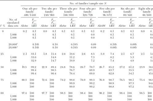
TABLE 3

Power comparison with results of Abecasiset al.(2000a, Table 4)

No. of families/sample sizeN

One sib per Two sibs per Three sibs per Four sibs per Five sibs per Six sibs per Eight sibs per

family: family: family: family: family: family: family:

480/1440 240/960 160/800 120/720 96/672 80/640 60/600

No. of F1,a, F1,a, F1,a, F1,a, F1,a, F1,a, F1,a,

simulated Fˆ1,a, Fˆ1,a, Fˆ1,a, Fˆ1,a, Fˆ1,a, Fˆ1,a, Fˆ1,a,

D⬘% data sets AbAw LRT AbAw LRT AbAw LRT AbAw LRT AbAW LRT AbAw LRT AbAw LRT

0 0.2 0.1 0.0 0.1 0.1 0.1 0.1 0.1 0.2 0.1 0.1 0.1 0.0 0.1

1,000 0.1 0.1 0.1 0.0 0.1 0.1 0.0

20,000a _0.105 _0.10 _0.105 _0.09 _0.105 _0.095 _0.09

20,000b _0.105 _0.10 _0.105 _0.09 _0.085 _0.085 _0.09

25 2.1 33.1 1.8 15.4 2.0 10.6 2.6 8.5 3.0 7.4 2.1 6.7 2.1 5.8

1,000 33.0 14.8 11.2 7.3 8.2 5.3 4.3

1,000 32.9 14.7 10.9 7.2 7.4 4.9 3.8

50 19.5 99.2 22.9 89.4 24.8 78.6 26.7 70.7 26.7 65.2 27.2 61.2 23.9 56.0

1,000 99.4 90.5 76.7 69.9 63.7 55.5 47.5

1,000 99.4 90.4 76.4 69.0 62.8 54.1 45.0

75 69.3 100 72.6 100 74.2 99.8 76.9 99.3 76.0 98.7 76.5 98.1 75.4 96.9

1,000 100 100 99.9 99.2 98.9 97.3 94.6

1,000 100 100 99.9 99.2 98.8 97.2 93.8

100 97.4 100 97.7 100 98.3 100 98.4 100 98.2 100 98.4 100 98.5 100

1,000 100 100 100 100 100 100 100

In the AbAw columns, the power (%) is taken fromAbecasiset al. (2000a, Table 4). In columns 4, 6, 8, 10, 12, 14, and 16

the power (%) ofF1,ais calculated on the basis of the theoretical approximation of noncentrality parameter␭1,aof test statistic F1,aat a 0.001 significance level; the empirical power (%) ofFˆ1,aand LRT are calculated as the proportions of 1000 or 20,000

simulated data sets that give significant results at the 0.001 significance level on the basis ofF1,a and the likelihood-ratio test

statistic, respectively. The parameters are the same as those ofAbecasiset al.(2000a, Table 4):q1⫽PM1⫽0.5,h

2_⫽_0.1,_␴2_⫽_100,

␴2

ga⫽10,␴2H⫽ ␴2Ga/2⫽30,␴2e⫽30. In addition,D⬘ ⫽DM1Q/DmaxandDmax⫽min(PM1,q1)⫺PM1q1. a_{Results of the row are calculated on the basis of}_Fˆ

1,a. b_{Results of the row are calculated on the basis of LRT.}

porate both parental and sibship phenotypes into the In Table 3, there is a trend that the power of (F1,a,

Fˆ1,a, LRT)␶to detect association decreases with the

in-models. This considerably increases the power as shown

in Table 3. creasing sibship sizes. This is partly because the sample

sizeNdecreases although the total number of offspring In Table 3, the first row of results corresponds to the

case when D⬘ is zero, i.e., a situation when the null is the same, 480: For 480 trio families of one sib per family, the total number of individuals isN⫽1440; for hypothesis of no association is true. Hence, the power

results for all these tests are simply the type I error rates. 60 families of eight sibs per family, the total number of individuals is N ⫽ 600. For the AbAw approach pre-It can be seen that the type I error rates are close to

the nominal level 0.001 ⫽ 0.1% when the number of sented inAbecasis et al.(2000a), the total number of offspring that are used in the model is the same, 480. simulated data sets is 20,000. This is consistent with the

conclusion of Table 2;i.e., the proposed model is robust. Since our models use phenotypes of both parents and offspring, the sample sizesNare different. On the other To make a comparison with the results ofAbecasis et

al.(2000a, Table 4), the results ofFˆ1,a and the LRT of hand, for the same total number of typed individuals

N, families of large sibship sizes contain less LD informa-1000 simulated data sets are also presented. In most

cases, the entries are equal to the nominal level 0.001⫽ tion than families of small sibship sizes. The readers may note that this result is consistent with findings in 0.1%;i.e., one of the 1000 data sets leads to a significant

(9)

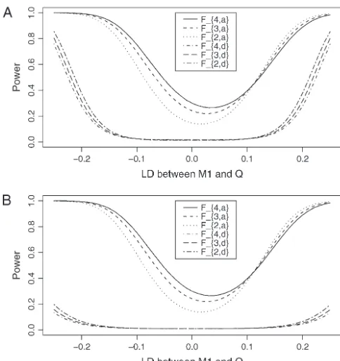
Figure2.—Power of test statisticsF4,a,F3,a,F2,a,F4,d,F3,d, and Figure1.—Power curves of test statisticsF4,a,F3,a,F2,a,F4,d,

F2,dagainst the heritabilityh2at a 0.01 significance level, when

F3,d, andF2,dagainst the measure of LD betweenM1andQat

q1⫽0.5,PMi⫽0.5,PMi⫽0.5,DMiQ⫽0.1,DMiMj⫽0.05,i,j⫽ a 0.01 significance level, whenq1⫽0.5,PMi⫽0.5,i⫽ 1, 2,

1, 2, 3, 4,i⬆j,␲12Q⫽0.5,␦12Q⫽0.25,␴2Ga⫽0.1 and sample

3, 4,DMiQ⫽0.08,i⫽2, 3, 4,DMiMj⫽0.05,i⬆j,␲12Q⫽0.5,

sizen⫽ 40, m ⫽ 30, s⫽ 20 for (A) a dominant mode of

␦12Q⫽0.25, heritability h2⫽0.15, polygenic effect variance

inheritancea⫽d⫽1.0 and (B) a recessive mode of

inheri-␴2

Ga⫽0.10 and sample sizen⫽40,m⫽30,s⫽20 for (A) a

tancea⫽1.0,d⫽ ⫺0.5, respectively. dominant mode of inheritancea⫽d⫽1.0 and (B) a recessive

mode of inheritancea⫽1.0,d⫽ ⫺0.5, respectively.

cance level for a dominant mode of inheritance (a ⫽ d⫽1.0) and a recessive mode of inheritance (a⫽1.0, to be more powerful than the family-based method for

d⫽ ⫺0.5), respectively. In addition to the merits shown the same number of individuals.

in Figure 1, the power of the test statisticsF4,a,F3,a,F2,a Comparisons of sample size and power of LD

map-is high when heritabilityh2_is_⬎_{0.10 for both modes of} ping:Power and sample size calculations are performed _inheritance.

to investigate the merits of the proposed method. Figure _{Figure 3 shows the power of test statistics}_F

4,a,F3,a,F2,a,

1 shows the power curves of the test statisticsF4,a, F3,a, _and_F

1,aagainst the trait allele frequencyq1(Figure 3A)

F2,a,F4,d,F3,d, andF2,dagainst the linkage disequilibrium _{or marker allele frequency} _P

M1 (Figure 3B) at a 0.01

coefficientDM₁Qat a 0.01 significance level for a

domi-significance level for an additive mode of inheritance nant mode of inheritance (a⫽d⫽1.0) and a recessive _a_⫽_1.0,_d_⫽_{0.0, respectively. The other parameters are} mode of inheritance (a ⫽1.0,d⫽ ⫺0.5). The related _{given in the Figure 3 legend. From Figure 3A, it can be} parameters are given in the Figure 1 legend. Generally, _{seen that the power of} _F

k,a increases as the trait allele

the power of F4,a using four markers in the model is _frequency_q

1increases. Figure 3B shows that the power

higher than that ofF3,a using three markers, which in _of_F_4,a_and_F_3,a_{is almost constant; in addition, the power}

turn is higher than that ofF2,ausing two markers. Hence, _of_F_2,a _{increases slowly, and the power of} _F_1,a _increases

multiple-marker analysis is advantageous. The power of _{as the marker allele frequency}_P

M₁increases. In general,

Fk,d is usually minimal unless the LD between locus Q _{the power of} _F

4,a and F3,a depends heavily on the trait

and markerM1 is very strong for the dominant mode _{allele frequency} _q

1, but not on the marker allele

fre-of inheritance. Note the power curves fre-of Figure 1 are

quencyPM₁. At first glance, it is strange that the power not symmetric with respect to DM₁Q. This is due to

ofF4,aandF3,adoes not depend very much on the marker

DM_iQ⫽0.08,i⫽2, 3, 4,DM_iM_j⫽ 0.05,i⬆ j, and so the

allele frequencyPM₁. The mystery is that the LD mea-power curves do not have to reach a minimum value _sures_D

M_iQ⫽ 0.125,i⫽2, 3, 4 are already high. That is whenDM₁Qis zero. Instead, they are shifted to the right, _{why the contribution of marker} _M

1 matters not very

so that the minimum is at a point whenDM1Q⬎0. Figure much to the power ofF2,a,F3,a, andF4,a. This adds one

2 provides the power of the test statisticsF4,a,F3,a, F2,a, more piece of information to the advantage of

multiple-marker analysis. That is, as long as some multiple-markers are

(10)

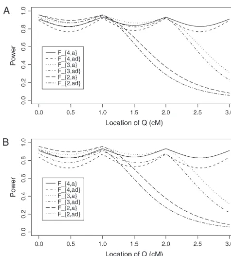
signifi-Figure4.—Power of test statistics F4,a, F4,ad, F3,a, F3,ad, F2,a, Figure 3.—Power of test statistics F4,a, F3,a, F2,a, and F1,a

andF2,adagainst location of QTLQat a 0.01 significance level.

against the trait allele frequencyq1(A) or marker allele

fre-The parameters are given by,q1⫽0.5,PMi⫽0.5,DMiQ(0)⫽ quency PM1 (B) at a 0.01 significance level for an additive

0.15,DMiMj⫽0.05,i,j⫽1, · · · , 4,i⬆j,␲12Q⫽0.5,␦12Q⫽ mode of inheritancea⫽1.0,d⫽0.0, whenPM1⫽0.5 orq1⫽

0.25, familial effect variance␴2

Ga⫽0.10, heritabilityh2⫽0.15

0.5, respectively. The other parameters are given byh2⫽_0.15,

and sample sizen⫽100,m⫽50,s⫽30, mutation ageT⫽

PMi⫽0.5,DMiQ⫽[min(PMi,q1)⫺PMiq1]/2, DM1Mi⫽[min

60 for (A) a dominant mode of inheritance a ⫽ d ⫽ 1.0

(PM1,PMi)⫺PM1PMi]/2,i⫽2, 3, 4,DMiMj⫽0.05,i,j⫽2, 3,

and (B) a recessive mode of inheritancea⫽1.0,d⫽ ⫺0.5,

4, i⬆j,␲12Q ⫽0.5, ␦12Q ⫽0.25, ␴2Ga⫽ 0.1 and sample size

respectively. MarkerM1locates at position 0 cM, marker M2

n⫽40,m⫽30,s⫽20.

locates at position 1 cM, markerM3locates at position 2 cM,

and markerM4locates at position 3 cM. The location of QTL

Qis along the horizontal axis;i.e., it moves from 0 to 3 cM.

in strong linkage disequilibrium with the trait locus, the power to detect the association is high.

Assume that the LD is due to historical mutationsT dominant mode of inheritance (a⫽d⫽1) and a reces-generations ago at QTL Q. At the initial generation sive mode of inheritance (a ⫽ 1.0,d ⫽ ⫺0.5), respec-when the mutation occurred, the LD coefficient is tively. The powers ofF4,a andF4,adwith four markers in

DMiQ(0)⫽P(MiQ)(0)⫺q1PMi, whereP(MiQ)(0) is the the model are generally high across the location of QTL

Q, since at least one marker is close to the QTLQ. The frequency of haplotype MiQ. The LD coefficient is

re-power ofF3,aandF3,adusing three markers in the model

duced by a factor 1⫺ ␪M_iQin each subsequent

genera-is similar to that of four markers, except that QTL Q

tion. The LD between marker Mi andQ isDM_iQ(T)⫽

locates far above marker M3, i.e., ␭M1Qⱖ 2.3cM. The

DM_iQ(0)(1⫺ ␪M_iQ)T at the current generation. Assume

power of F2,a andF2,ad using two markers in the model

that the markerM1locates at position 0 cM, markerM2

is high when the QTL is close to markers M1 andM2.

locates at position 1 cM, markerM3locates at position

However, once the QTL is far above marker M2 (i.e.,

2 cM, and markerM4 locates at position 3 cM. Under _␭M

1Qⱖ1.3cM ), the power of F2,a and F2,ad using two

the assumption of no interference, we may calculate the

markers in the model decreases very quickly. Figure 4 recombination fraction ␪M_iM_j⫽[1⫺exp(⫺2⍀M_iM_j)]/2

implies that multiple-marker LD analysis has high power by Haldane’s map function, where ⍀M_iMj is the map _{in fine mapping of QTL. Moreover, the power of test}

distance between markerMiand markerMj. Similarly, _statistic_F

k,a, which tests only the additive effect, is higher

the recombination fraction ␪M_iQ can be calculated by _{than that of}_F

k,ad, which tests both the additive and

domi-the distance⍀M_iQbetween QTLQand markerMi,i⫽ nance effects through the proposed model. The reason is that the degrees of freedom of test statistics increases 1, · · · , 4. Suppose that the QTLQis located along the

horizontal axis;i.e., it moves from 0 to 3 cM. Figure 4 if the dominance effect is added to the test statistics. Figure 5 shows the power curves of test statistic F4,ad

shows the power curves of the test statisticsF4,a,F4,ad,F3,a,

(11)

F4,aandF3,ais⬍500 and that ofF2,ais⬍700 if heritability

h2 _is ⬎_{0.1. The required number of families of test}

statistics F1,a is very large for both favorable and less

favorable cases.

AN EXAMPLE

The proposed method is applied to the Genetic Analy-sis Workshop 12 German asthma data (Meyers et al.

2001). The data consist of 97 nuclear families, including 415 persons. Seventy-four families have two children, 19 have three children, and 4 have four children.Wjst

et al. (1999) perform linkage analysis for total serum

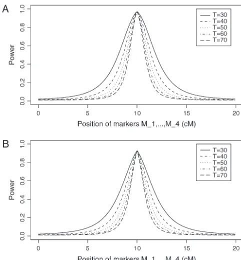
IgE by a nonparametric statistic of MAPMAKER/SIBS 2.1. Three markers on chromosome 1 are shown to be linked with immunoglobulin E (IGE) level,i.e., marker D1S207 at position 118.1 cM, marker D1S221 at position 146.7 cM, and marker D1S502 at position 151.2 cM. In FanandJung(2003), we analyze the data using sibships and confirm the result of Wjst et al. (1999). By the method proposed in this article, we analyze the data again. The dominance variance of log(IGE) is signifi-cantly⬎0 at position 149.85 cM (P-value, 0.00075; com-Figure5.—Power of test statisticF4,adfor mutation ageT⫽

30,T⫽40,T⫽50,T⫽60,T⫽70 against position of markers pared with theP-value of 0.01 inFanandJung2003).

Mi, i⫽ 1, · · · , 4 at a 0.01 significance level. The QTLQ On this basis, we collapse alleles 6, 8, and 10 as allele

locates at position 10 cM. The four markers flank the trait _M

1at marker D1S207 and others as allelem1. At marker

locusQ; two markers are on each side of the QTL with equal

D1S221, alleles 5, 6, and 7 are collapsed as allele M2

distance to each other as follows:M2⫽5⫹M1/2,M3⫽15⫺

and other alleles as allele m2. At marker D1S502, we

M1/2, M4⫽ 20 ⫺ M1. q1 ⫽ 0.5,PMi⫽0.5, DMiQ(0)⫽0.15,

collapse alleles 7, 8, and 12 as alleleM3 and others as

DMiMj⫽0.05, i, j ⫽1, · · · , 4,i ⬆j, heritabilityh

2⫽ _0.15,

allelem3. Then, we find that coefficient␦2is significantly

polygenic effect variance␴2

Ga⫽0.1 and sample sizen⫽40,

m⫽30,s⫽20 for (A) a dominant mode of inheritancea⫽ different from 0 at position 149.85 cM, with aP-value

d⫽1.0 and (B) a recessive mode of inheritancea⫽1.0,d⫽ _{of 0.034 by likelihood-ratio test (compared with the}_P

-⫺0.5, respectively. _{value of 0.0475 in}_Fan _and _Jung _{2003) and a} _P_-value

0.034 by F-test (compared with the P-value 0.0484 in FanandJung2003). The estimation is␦ˆ2⫽0.76. Hence,

mutation age at a 0.01 significance level. The trait locus

we are able to confirm the result ofWjstet al.(1999) and

Qlocates at position 10 cM. The four markers flank the

find that marker D1S221 is associated with log(IGE). trait locusQ; two markers are on each side of the QTL

Compared with the results ofFan andJung (2003), with equal distance to each other as follows:M2⫽5⫹

the evidence in the above paragraph is stronger since

M1/2, M3 ⫽ 15⫺ M1/2, M4 ⫽ 20⫺ M1. Here Mi also

theP-values are smaller. There are two reasons for this. denotes the location in centimorgans of markerMi. As

In this article, all family members are used in the analysis the mutation ages, the power decreases and the power

(compared with only sibships used in Fan and Jung can be high only when the markers are close to the trait

2003). This article used three markers in the analysis locus.

(compared with only two markers used inFanandJung Figure 6 shows the required number of trio families

2003). Hence, the proposed model improves the perfor-or families with both parents and two offspring fperfor-or the

mance of the previous method. test statisticsF4,a,F3,a,F2,a, andF1,aagainst heritabilityh2

at a significance level 0.01 and power 0.8. For a favorable

case (Figure 6, A and C), the parameters are given by DISCUSSION

q1⫽ PMi⫽0.5, DMiMj⫽0.05, andDMiQ⫽0.1 for i,j ⫽ _{On the basis of multiple diallelic markers, this article}

1, · · · , 4,i⬆ j. For a less favorable case (Figure 6, B _{proposes variance component models for} high-resolu-and D), the parameters are given by q1 ⫽ 0.2, PM_i⫽ _{tion joint linkage and association mapping of QTL . The} 0.8,DM_iM_j⫽ 0.0, andDM_iQ⫽ 0.03 fori,j ⫽ 1, · · · , 4, models extend our previous work using two diallelic markers in analysis and incorporate genetic-marker

in-i⬆ j. For the favorable case, the required number of

families of test statisticsF4,aandF3,ais⬍200 and that of formation into the models (FanandXiong2002, 2003; FanandJung2003;Fanet al.2005). By analytical

analy-F2,ais⬍600 if heritabilityh2is⬎0.1. For the less favorable

(12)

Figure6.—Sample size of test statisticsF1,a,

F2,a,F3,a, andF4,aagainst heritabilityh2at a 0.01

significance level and 0.80 power for a

domi-nant mode of inheritancea⫽d⫽1.0. For a

favorable case (A and C),q1⫽ 0.5,PMi⫽0.5,

DMiMj⫽0.05,DMiQ⫽0.1,i,j⫽1, 2, 3, 4,i⬆j; for a less favorable case (B and D),q1⫽0.2,

PMi⫽0.8, DMiMj⫽0.0, DMiQ⫽0.03, i, j ⫽ 1, 2, 3, 4,i⬆j. In addition, the polygenic effect variance␴2

Ga⫽0.1.

genetic effects are incorporated in the mean coeffi- may have higher power than models that use less mark-ers. Multiple-marker analysis can be more advantageous cients. On the basis of marker information, a multipoint

interval mapping method is provided to estimate the and has higher power in fine mapping QTL.

In an association study, population stratification can proportion of allele-sharing IBD and probability of

shar-ing two alleles IBD at a putative QTL for a sib-pair. have a huge impact on a study, which leads to high false positives (EwensandSpielman1995).ZhaoandXiong It is shown that recombination fractions, i.e., linkage

information, are contained in variance-covariance ma- (2002) proposed unbiased quantitative population asso-ciation tests to investigate the issue. In this article, we trices. Therefore, the proposed methods model both

association and linkage in a unified model. perform type I error calculations. We allow for the very extreme form of population admixture, in which each In the literature, there is plenty of research for linkage

mapping of QTL (Amos 1994; Fulker et al. 1995; family is drawn from a different stratum (Abecasis et al. 2000a). Type I error rates of the proposed test statis-Almasy and Blangero 1998). The linkage evidence

can be detected by fitting model (6) as the first step on tics are calculated to investigate the behaviors of the test statistics under the null distribution. Five test cases the basis of a sparse genetic map. In this article, we put

more effort into high-resolution linkage disequilibrium including population admixture are considered to in-vestigate the type I error rates. The results show the mapping of QTL in the presence of prior linkage

evi-dence. To test the association between the trait locus proposed models and methods have correct type I error rates for most cases and are robust.

and the markers, both likelihood-ratio tests andF-tests

can be constructed on the basis of the proposed models. In a QTL mapping study, a strategy may be taken as follows. First, linkage analysis can be carried out using In addition, analytical formulas of noncentrality

param-eter approximations of theF-test statistics are provided. a sparse genetic map. Then, an association study can be performed using a dense genetic map for high-reso-After comparing it with the AbAw approach, it is found

that the method proposed in this article is more power- lution mapping of the trait. The basic idea is to take advantage of linkage analysis for prior linkage informa-ful and advantageous on the basis of simulation study