Empirical threshold values for quantitative trait mapping.

(1)

Copyright 0 1994 by the Genetics Society of America

Empirical Threshold Values for Quantitative Trait

Mapping

G .

A. Churchill

and R.

W.

Doerge

Biometrics Unit, Cornell University, Zthaca, New York 14853

Manuscript received April 22, 1994

Accepted for publication July 25, 1994

ABSTRACT

The detection of genes that control quantitative characters is a problem of great interest to the genetic

mapping community. Methods for locating these quantitative trait loci (QTL) relative to maps of genetic

markers are now widely used. This paper addresses an issue common to all QTL mapping methods, that

of determining an appropriate thresholdvalue for declaring significant QTL effects. An empirical method

is described, based on the concept of a permutation test, for estimating threshold values that are tailored

to the experimental data at hand. The method is demonstrated using two real data sets derived from F2

and recombinant inbred plant populations. An example using simulated data from a backcross design

illustrates the effect of marker density on threshold values.

M

ETHODOLOGICAL research on the problems of

detecting and locating quantitative trait loci (QTL) has received considerable attention over the past several years. A variety of methods have been developed to analyze quantitative trait data (WELLER 1986, 1987; LANDER and BOTSTEIN 1989; HALEY and b o r r 1992; KNon and m y 1992; HALEY et al. 1994; &ONELL

et al. 1992;J~~sEN 1993a,b;JmS~~ and STAM 1994; ZENG 1993,1994). A problem common to all of these methods is the difficulty of determining appropriate significance thresholds (critical values) against which to compare test statistics (usually LOD scores or likelihood ratios) for the purpose of detecting QTL. The source of this difficulty is twofold. First, there is the problem of determining (or approximating) the distribution of the test statistic under an appropriate null hypothesis. In most cases, the regularity conditions that ensure an a s ymptotic chi-square distribution for the likelihood ratio test statistic are not satisfied (GHOSH and SEN 1985; HARTIGAN 1985; FENG 1990). There are often additional problems due to finite sample sizes and distributional properties of the quantitative trait that might cause one to doubt the reliability of asymptotic approximations. The second source of difficulty is the multiple hypothesis testing that is implicit in the genome searches used for locating QTL ( m y1994; JANSEN 1993a,b; JANSEN and STAM 1994; ZENG 1993, 1994). A large number of tests may be carried out, many of which are not independent. The dependence structure of these tests is difficult to analyze in cases other than the extremes of very dense or very sparse genetic maps. Elegant theoretical arguments have been presented (LANDER and BOTSTEIN 1989) that address both of these issues. However, they offer the user formulas for threshold values that are unfortunately difficult to apply and are based on a number of assumptions that are not likely to be met in practice (LANDER and BOTSTEIN 1989).

Genetics 138: 963-971 (November, 1994)

The problem of determining appropriate threshold values is made even more difficult because there are many factors that can vary from experiment to experiment and can influence the distribution of the test statistic. These include, but are not limited to, the sample size, the genome size of the organism under study, the genetic map density, segregation ratio distortions, the proportion and pattern of missing data, and the number and magnitude of segregating QTL. Our goal in this work is to provide researchers involved in QTL mapping projects with a simple and intuitive procedure for estimating a threshold value and thus detecting significant QTL effects. Any such procedure must be statistically sound and should reflect, to the greatest extent possible, the characteristics of each particular experiment. In this paper, we describe a method based on the concept of permutation tests as first proposed by FISHER (1935). It involves repeated “shuffling” of the quantitative trait values and the generation of a random sample of the test statistic from an appropriate null distribution. The procedure is statistically valid when used in conjunction with likelihood or regression based test statistics and for

any distribution of the quantitative trait. Because our procedure is empirical, based on the observed marker and trait data, it will automatically reflect the characteristics of the particular experiment to which it is applied.

Before proceeding to describe our method, we review the usual “QTL hypotheses” and discuss a handful of previous studies on the QTL detection problem, realizing that by no means are we presenting a complete literary synopsis of this field.

(2)

and W.

It is usual but not necessary to assume that, within classes defined by the (unknown) QTL genotype, the quantitative trait is normally distributed. Under the null hypothesis Hh, the trait values should follow a single normal distribution. Thus any association between the trait values and a marker (interval) in the genetic map will be due purely to chance effects. Under the null hypothesis

@, the trait should follow a normal mixture distribution with mixing proportions equal to %. Again any associations between the trait values and markers unlinked to the QTL are due to chance. Under the alternative hypothesis HA, the trait should follow a normal mixture distribution with mixing proportions determined by the recombination fraction between the marker (interval) and the QTL. In this case, real associations between the trait values and the marker(s) are expected (DOERGE 1993).

The most widely used algorithm for QTL detection and mapping is that implemented in the MAPMAKER/ QTL software package (PATERSON et al. 1988; LINCOLN and LANDER 1992; LINCOLN et al. 1992) as first described by LANDER and BOTSTEIN (1989). Their method is based on LOD scores (equivalent to log likelihood ratios) computed at regular incremental values throughout the genome. Although the null hypothesis assumed by MAPMAKER/QTL algorithm is HA, the null hypothesis of an unlinked QTL @ is discussed in Appendix A4 of LANDER and BOTSTEIN (1989) as being more appropriate in some cases. An eloquent argument based on an Orenstein-Uhlenbeck diffusion process is used to determine the distribution of the maximum LOD score (over the entire genome) under the null hypothesis. Propo- sition 2 along with its Corrigendum (LANDER and BOTSTEIN 1994) describes the calculation for determining the threshold value taking account of the known chromosome number and the known genetic length of the organism. LANDER and BOTSTEIN (1989) suggest that a typical LOD threshold should be between 2 and 3, to

ensure an overall false positive (type I error) rate for QTL detection of 5%. LANDER and BOTSTEIN (1989) also

show how to estimate threshold values based upon simulated data.

KNOTT and HALEY (1992) used simulations to study the distributional properties of likelihood ratio tests for QTL detection. Their results suggest that the chi-square approximation to the distribution of likelihood ratio test statistics is not reliable in many cases and is at least ques- tionable in every case. The problem of determining a significance threshold value for multiple nonindepen- dent tests is not addressed in detail, but the reader is

cautioned to consider setting higher significance thresholds in this case. In their conclusion & O n and HALEY

(1992) suggest that further theoretical work is needed in this area as no alternative other than simulation is presently available for setting significance thresholds.

CARBONELL et al. (1992) note that it is inappropriate to use standard chi-square approximations for threshold

values. They consider two different chi-square based thresholds and compare them to determine which gives “better” results. They also conclude that more research is needed to determine appropriate threshold values.

ZENG (1993) presents a regression based method that includes other markers as cofactors in a multiple regression. He advocates the use of an approximate one degree of freedom chi-square threshold for his method when the sample size is large, and the number of evenly spaced markers is small. Realizing that representative threshold values reflect the sample size, the number of markers in the model and the size of the marker interval, ZENC (1994) relies on a simulation study to explore these issues in a genome of unevenly markers and small sample size. For small sample size, the reader is cautioned as to the number of markers allowed in the model, since too many fitted markers can substantially increase the threshold value of the test statistic. To this point ZENG offers no effective solution to the threshold problem other than to suggest using computer simulation.

Notably, computer simulation has been used as a means of estimating threshold values (LANDER and BOTSTEIN 1989). Unfortunately simulation based tests are model dependent and rely heavily on the assumptions from which the data are simulated. The validity of parametric and nonparametric based threshold values is detailed in the DISCUSSION.

Other researchers (KNMP et al. 1990; JANSEN 1993b) have advocated the use of “conservative” threshold values based on chi-square distributions with either one or two degrees of freedom. The method presented by JANSEN and STAM (1994) relies on weighted sum of squared residuals for the case of mixture models. Ad- mittedly, JANSEN and STAM (1994) state, “as an ad hoc approximation we used the chi-squared distribution with one degree of freedom, multiplied by the residual variance.” No justification is given for determining threshold values in this manner.

The difficulties in determining an appropriate asymp totic distribution are not too surprising when one con- siders that the most widely used hypothesis test com- pares a mixture distribution under HA to a non-mixture distribution under H;. It is well documented ( e . g . , HARTIGAN 1985; GHOSH and SEN 1985) that the usual asymptotic arguments do not apply in this case as the hypotheses are not properly nested. The fact remains that these hypotheses are of significant practical importance and thus we are highly motivated to study this problem further.

METHODS

Motivation: Data for quantitative trait analysis consist

(3)

Empirical Threshold Values 965

marker and, if the markers are organized into a genetic map, at regularly spaced increments in the intervals between markers. We refer to the location at which a test statistic is computed as an analysis point. In a single marker analysis, all of the analysis points are markers. If analysis points between markers are used, the analysis is an interval analysis. If there is a QTL effect at a specific location in the genome there will be an association between the trait values and the analysis points linked to that location. This association may be detected by t tests or ANOVA ( SCHEW 1959) in a single marker analysis or by likelihood ratios in an interval analysis. If there is no QTL effect linked to a marker, any associations between the trait values and the marker are likely to be weak and attributable to chance effects. Thus the key to detecting QTL effects is the detection of significant associations between the phenotypic trait values and the markers and/or intervals in a genetic map.

Our approach to the estimation of a significance threshold is based upon this simple observation of marker-phenotype association. It can be applied to single marker or interval mapping approaches using any test statistic with power to detect associations. If the data indicate that there are QTL effects, we can effectively destroy any association between the trait values and the analysis points linked to the QTL by randomly shuffling the trait values, i . e . , by reassigning each trait value to a new individual while retaining the individual’s genetic map. On the other hand, if there are no QTL effects linked to specific regions of the genome, randomly shuffling the trait values across individuals will not alter the distribution of the test statistic. Any associations should still be small and attributable to chance. If we compute the value of an appropriate test statistic at each analysis point in the shuffled data sets, we are essentially sampling from a null distribution corresponding to the hypothesis of no associations between the trait values and the genetic maps.

As

the genetic maps and trait values are not altered by the shuffling procedure, this distribution will automatically take into account the particular characteristics of the experiment at hand.

Threshold estimation: Individuals in the experiment are indexed from 1 to n. The data are shuffled by com- puting a random permutation of the indices 1,

. .

., n

(FISHER 1935) and assigning the ith trait value to the individual whose index is given by the ith element of the permutation. The shuffled data are then analyzed for QTL effects. The resulting test statistics at each analysis point are stored and the entire procedure (shuffling and analysis) is repeated N times. At the end of this process we will have stored the results of QTL analyses on N shuffled data sets. Two types of threshold values can be estimated from these results. The first is a comparisonwise threshold that can be estimated separately for each analysis point and provides a 100( 1 - a) % critical value for the test at that point. One should realize that since

the same sample of permutations is used for each analysis point in a specific repetition, the comparisonwise threshold values will be correlated. In order to eliminate this correlation one could consider doing a permutation of the trait values at each analysis point, but this soon becomes computationally undesirable. The second type of critical value is an experimentwise threshold that provides an overall 100( 1 - a) % critical value that is valid simultaneously for all analysis points. Results of the QTL analysis on the original data can be compared to these critical values to determine statistical significance and thus to detect QTL effects.

A comparisonwise critical value is obtained by ordering the N test statistics obtained at each analysis point in the map and finding their 100( 1 - a) percentile. For example, if a comparisonwise significance level of a =

0.05 is desired and N = 1000, the 950th value of the ordered test statistics will be our estimate of the comparisonwise critical value at that analysis point. Using this critical value to define a test controls the type I error rate at that point to be a or less. One should keep in mind that many individual tests may be computed and each presents a new opportunity to make a type I error. Thus if we use comparisonwise critical values, the type I error rate over the entire genome may be much higher than a.

The experimentwise critical value may be obtained by first finding the maximum test statistic over all analysis points for each of the N shuffled analyses. These values are then ordered and their 100( 1 - a) percentile is our estimated experimentwise critical value. The experimentwise critical value is used to detect the presence of a QTL somewhere in the genome while controlling the overall type I error rate to be a or less. The experimentwise critical value will necessarily be higher than the comparisonwise values, thus the price for controlling the type I error rate over the entire genome is some loss of power to detect QTL effects.

An obvious question at this point is “How large should N be?” We recognize that this procedure may be mod- erately expensive in computer time. Larger values of N will provide more precise estimates of the critical values. Thus there is a tradeoff here. Based on our limited ex- perience with this procedure, we recommend that at least 1000 shuffles be used for estimating critical values at a = 0.05. For more extreme critical values such as a = 0.01, as many as 10,000 shuffles may be needed to obtain stable estimates.

Justification: The simple nature of the shuffling pro-

(4)

theory of permutation testing is provided by &OD (1994).

A permutation test in the simplest case is used to detect a location shift in data that are divided into

mo

sets of observations Z = ( X , ,

. . .

, X,, Y,,

. . .

, Y , ) . The test is performed by enumerating all permutations of the observed data z' E S( z) (where S ( x ) denotes the set of

all permutations of z) and ordering them by the values of a function h ( z ' ) which is usually the likelihood of the data under an alternative hypothesis. The null hypothesis of no shift in location is rejected if the value of the function h ( z ) based on the observed data is among the k largest values of h ( z ' ) based on the permuted data where k = [an!], and [x] denotes the greatest integer not greater than x. In practice the number of permutations is usually too large to enumerate. However, one can compute an approximate permutation test by generating a random sample from the set of all permutations of the data. For a random sample of size N, the estimated critical value is the kth largest value of h ( z ' )

where k =

l a w .

Consider testing for QTL effects at a single marker locus in a backcross population with a single segregating QTL. Let

{

i

0 non-recurrent parental allele

Q i = 1 non-recurrent parental allele

is absent at the QTL

is present at the QTL

and

0 non-recurrent parental allele

1 non-recurrent parental allele is absent at the marker

is present at the marker

M i

=

for individuals i = 1,

. . .

, n. Let

Yi

be the phenotypic trait value of the ith individual. We will assume the trait value is a random variable with (conditional) density function

p,,

p( y,O) = f( y ) within the class of individuals defined by Q. = 0 and with density function

p,,

4( y, 1)

= f( y - A) within the class of individuals defined by

Q = 1. Thus the effect of the non-recurrent parental allele is to shift the density function of the trait by an amount A. We will assume, without loss of generality, that A > 0. Of course, the QTL genotype cannot be di- rectly observed. For a given marker linked to the QTL with recombination fraction r (0 5 r 5 %), the conditional densities for the trait values are

p,,

M( y, m) = ~ ~ ( 1 -

4""fC

y)

+

6 - V -

4"f(

y - 4 . (1)

The mixture form of the density arises because the true QTL state is unknown. The essential points for our justification are (1) when A > 0 and r< 95, PYlM( y,l) is stochas- tically larger than

p,,,(

y,O) and (2) when A = 0 (corresponding to Hi) or when r = M (corresponding to

Po),

the

two conditional density functions,

p,,

M ( y,O) and

p,,

M ( y,l)

,

are equal. Now let

n

Nym)

=

n

P,,

d y , , mil (2) I= 1

wheref( ) is taken to be a normal density function, y = y,,

. .

.

, y, and m = m,,

. . .

, m,. Thus h( ) is the likelihood function under the alternative hypothesis HA as- suming the trait values are normally distributed within QTL genotype classes. Note that because h( ) is used only to order the permutations, any monotone transformation of h( ) such as the log likelihood, log likelihood ratio or LOD score will yield an equivalent test. With this choice of h( ) and points (1) and (2) above, the conditions of Lemma 3 in LEHMANN (1986, p. 234)

are satisfied. It follows that the permutation test is unbiased. That is, it has a type I error rate equal to a under either of the null hypotheses Hi or and it has power greater than a for any alternative satisfying point (1)

above. Furthermore, in the case where the true distribution of the phenotypic trait within the QTL genotype classes is normal, the permutation test is most powerful.

We note that the permutation test applied to a single marker is the non-parametric analog of a t test. Although the t test has proven to be robust, the conditions for a t test are not satisfied in this case (DOERCE 1993) and the permutation test may be more appropriate. When the trait distribution is not normal within QTL genotype classes, the permutation test is still unbiased. In this case, a more powerful test could be derived by introducing the true density function

f(

) for the trait values into Equations 1 and 2. However, we note that the permutation test is robust to distributional assumptions and when applied with a normal density function f( ) will generally lose very little power (Box and ANDERSON 1955).

This justification of the permutation test can be ex- tended to analysis points within an interval. The mixtures in (1) are slightly more complex (DOERGE 1993)

but the stochastic ordering of the densities will still hold. In the case of F, and other experimental crosses, the numbers of QTL genotype classes may be increased again making the mixtures in (1) more complex. The permutation test will still be unbiased for any form of the additive and dominance effects. However, because there are more than two marker classes, simple one-sided tests of location shift cannot be constructed and most powerful unbiased tests do not exist (LEHMANN 1986).

To apply the permutation test to the whole genome (experimentwise threshold), we consider a new function

h( ) which is the maximum of the likelihood over all analysis points. The conditions of Lemma 3 (LEHMANN

(5)

Empirical Threshold Values 967

TABLE 1

Estimated threshold values for MAPMAKER/QTL sample data

1 - CY Experimentwise Comparisonwise” Critical valueb

0.90 2.07 1.01 0.5885

0.95 2.51 1.34 0.8339

0.99 3.24 2.13 1.4397

Values based on LOD scores from 1000 permutations of the origi-

”

Average across all analysis points. b

nal data.

M ~oglLlex:l,.

EXAMPLES

MAPMAKER sample data: We have applied the permutation test to the F, data that are distributed with MAPMAKER l . l b software (PATERSON et al. 1988; LINCOLN and LANDER 1992; LINCOLN et al. 1992). The file

sample.raw contains phenotypic trait data on 333 individuals and their genotypes at 12 marker loci. We used the linkage groups and map distances as established by

the MAPMAKER/EXP 3.0 manual (LANDER and GREEN

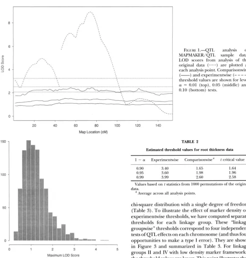
1987; LINCOLN and LANDER 1992; LINCOLN et al. 1992). The trait values were transformed by taking their loga- rithm for purposes of comparison with the sample analysis. (Transformation to obtain “normality” is not necessarily correct or even possible in some cases as the expected distribution of a trait in the presence of a QTL effect is a mixture distribution.) The trait values in sam- ple.raw were shuffled and the usual QTL analysis was performed using MAPMAKER/QTL. This process was repeated 1000 times and the LOD scores at each 2 c M increment analysis point were stored. To obtain comparisonwise threshold values, the 1000 LOD scores at each analysis point were sorted and the 100( 1 - a) percentile value was located. The results are summarized in Table 1 and in Figure 1. We see in this experiment that the comparisonwise threshold values are fairly constant across the two linkage groups. This need not be the case. Fluctuations in these values (shown in Figure 1 ) are due in part to the sampling of the permutation set. They are larger for the more extreme critical values (e.g., 1 -

a = 0.99) that are not as precisely estimated. Also note that the 95% LOD score threshold values are on average about 1.34. This LOD score can be rescaled to a likelihood ratio test statistic (divide by log,,( e)/2 = 0.2171). The result 6.17 is slightly greater than the chi-square critical value on 2 d.f., = 5.99. To obtain the experimentwise threshold, we first identifjr the maximum peak for each of the 1000 QTL analyses and then sort these values to obtain the l O O ( 1 - a) percentile (see Table 1 ) . The peak LOD score obtained on the original (not shuffled) data is 8.926, clearly indicating a significant QTL effect. There is a notable difference between the permutation based threshold values and the critical values based upon a chi-square distribution with a single degree of freedom (Table 1 ) . A histogram of the 1000 maximum LOD scores is shown in Figure 2. The distri-

bution is seen to be right skewed as is typical for distributions of extreme values.

Single marker analysis of recombinant inbred data: In this example, we consider a recombinant inbred (F,) population of rice derived from a cross between C039 (maternal) and Moroberekan. A total of 203 recombinant inbred lines were scored at 147 molecular markers. The quantitative trait of interest is root thickness (in micrometers) (M. C. CHAMPOUX, G . WANG, S. SARKARUNG, D. J. MACKILL, J. C. T TO OLE, N. HUANG and S. R. MCCOUCH, UNPUBLISHED RESULTS).

Application of the permutation test to these data illustrates two points. First, it was noticed that the segregation ratios in this population are severely skewed and the experimentwise threshold values for QTL detection should reflect this peculiarity of the data. Second, interval mapping software for the analysis of RI populations is not readily available. Therefore, we have carried out a single marker analysis using a t test at each analysis point (marker). We note that the assumptions of a t test are not satisfied in this case.

The original data were permuted 1000 times and the

t statistics at each of the 147 markers were recorded. Comparisonwise thresholds were estimated for each of these tests (not shown). The degrees of freedom for each t test vary slightly from marker to marker due to missing data. The averages of all 147 comparisonwise thresholds are summarized in Table 2. Note that they compare very well with the corresponding t distribution critical values. Experimentwise thresholds are of more interest in this example. The maximum t test statistic (across all markers) from each of the 1000 permutations were used to obtain the experimentwise threshold. Re- sults are summarized in Table 2. The maximum t test statistic for the original data was 9.0350, indicating a significant QTL effect in these data.

To determine if 1000 permutations of the data are sufficient to estimate experimentwise thresholds, we repeated the entire experiment 10 times. Standard errors of 0.028, 0.020 and 0.061 for the estimated threshold values were obtained at a = 0.10,0.05 and 0.01, respec- tively. This suggests that 1000 permutations were ad- equate for estimating critical thresholds at a = 0.10 and 0.05. More extreme type I error rates such as a = 0.01 may require larger numbers of permutations to yield threshold estimates accurate to two decimals.

A simulated example: One hundred backcross individuals were simulated in a genome containing four chromosomes of 100 cM each. Chromosomes

Z

and

ZZZ

(6)

968

8

6

8

3 4

a,

0-J

D

2

0

150

-

100

-

50

-

".

20 60 40

80 120 100 140

Map Location (cM)

P

0

L""

"

0 1 2 3 4 5

Maximum LOD Score

FIGURE 2.-Histogram of maximum LOD scores for

MAF"AKER/QTL sample data. The maximum LOD score across all analysis points was computed for each of 1000 permutations of the original data. Percentiles of this distribution are used to define experimentwise threshold values.

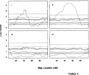
(a2 = 1.0) was simulated at 61.6 cM from the left end of chromosome II.

Each of the 1000 permuted data sets was analyzed in MAI"AKER/QTL under the backcross data type. Com- parisonwise thresholds for the LOD scores are shown in Figure 3 and the average values are summarized in Table 3. Note that the comparisonwise values are fairly constant throughout the entire genome (Figure 3), and agree fairly well with the threshold values based upon a

FIGURE I.-QTL analysis of

MAPMAKER/QTL sample data. LOD scores from analysis of the original data (...) are plotted at each analysis point. Comparisonwise

(-) and experimentwise (-

- -

-)

threshold values are shown for level cy = 0.01 (top), 0.05 (middle) and 0.10 (bottom) tests.

TABLE 2

Estimated threshold values for root thickness data

1

-

a Experimentwise Comparisonwise' 1 critical value

0.90 3.40 1.65 1.64

0.95 3.60 1.98 1.96

0.99 3.99 2.60 2.58

Values based on f statistics from 1000 permutations of the original

" Average across all analysis points. data.

chi-square distribution with a single degree of freedom (Table 3). To illustrate the effect of marker density on experimentwise thresholds, we have computed separate thresholds for each linkage group. These "linkage groupwise" thresholds correspond to four independent tests of QTL effects on each chromosome (and thus four opportunities to make a type I error). They are shown in Figure 3 and summarized in Table 3. For linkage groups I1 and

IV

with low density marker frameworks, the threshold values are lower. This point illustrates that the estimated threshold values do indeed reflect the characteristics of the experiment (chromosome) to which they are applied. We note also that the thresholds for chromosomes I and II that contain QTL are essentially identical to thresholds for chromosomes IIIand N

that do not contain QTL. This last point illustrates that the shuffling effectively breaks up any association of QTL effects and markers.

DISCUSSION

(7)

Empirical Threshold Values 969

I I I I

3

4

1

111

... ...

I

""" -,

,""

_'."""".""-

FIGURE 3.-QTL analysis of simulated backcross data. The figure is divided into four sec- tions corresponding to the four linkage groups. Each linkage groups is 100 cM in length. Link- age groups I and I1 contain QTLs. Linkage groups 111 and IV do not. Linkage groups I and

111 are mapped at high density (50 markers each) and linkage groups I1 and IV are mapibed at low density (10 markers each). LOD scores

from analysis of the original data (*....) are plotted at each analysis point. Comparisonwise

(-) and linkage groupwise (-

-

-) threshold values are shown for level a = 0.01 (top), 0.05 (middle) and 0.10 (bottom) tests.

20 40 60 80 20 40 60 80

Map Location (cM)

TABLE 3

Estimated threshold values for the simulated backcross data

Experimentwise Comparisonwise Critical value

1-Cu L G l b LC2 LG3 LG4 TGC LG1 LG2 LG3 LG4 TG % 10g,oex:1,

0.90 1.45 1.29 1.48 1.31 1.98 0.58 0.61 0.59 0.61 0.60 0.5885

0.95 1.83 1.57 1.84 1.59 2.27 0.84 0.87 0.85 0.86 0.85 0.8339

0.99 2.44 2.21 2.51 2.19 2.99 1.48 1.43 1.51 1.45 1.48 1.4397

Values based on LOD scores from 1000 permutations of the original data. a Average across all analysis points in the linkage group.

LG = linkage group.

'TG = total genome.

constructing tests are available but none seem to offer the broad advantages of permutation tests.

Parametric tests ( e . g . , t test) based on a sampling model are often most powerful when the data are known to follow a particular distribution. In some cases exact distributions for the test statistic can be derived from the model. In other cases large sample (asymptotic) a p proximations to the distribution can be derived. We have noted above the difficulties with these approaches when applied to the QTL hypotheses. Parametric tests can also be developed on the basis of simulated data

(BIRNBAUM 1974). However, simulation based tests are highly dependent on the model assumptions for their validity. Permutation tests, on the other hand, are valid under very mild conditions (exchangeability under H,) and thus provide protection against failures of the model assumptions. They are at least as powerful as the best unbiased parametric tests when the model assumptions hold.

The nonparametric bootstrap procedure (EFRON 1979) could also be used to construct a test of QTL hypotheses at an analysis point by resampling with replace- ment the phenotypes within each marker class. Boot-

strap tests in this case are asymptotically equivalent to permutations tests. However in finite samples, the bootstrap test cannot be guaranteed to provide a conservative type I error rate nor can it be guaranteed to be most powerful. It is not clear how one would apply the bootstrap procedure to construct a global test for QTL effects analogous to permutation tests based on experimentwise thresholds.

We have presented a method of estimating threshold values for declaring significant QTL effects in a genome or at any point within a genome by the application of a permutation test. The test is valid for any continuously distributed trait, i . e . , it will have the correct type I error level and will have power to detect QTL effects under the alternative hypothesis HA' The threshold values ob-

(8)

970 G . A. Churchill and W. Doerge

investment compared to the many hours required to xore and genotype individuals in a typical QTL experiment.

Generalizations of the permutation test to the problem of detecting multiple QTL effects may be possible. LEHMANN (1986) notes that in the case of a heteroge- neous population, the power of a permutation test can often be improved by stratifying the population accord- ing to factors unrelated to the treatment of interest but known to affect the outcome (analogous to unlinked QTL). In the case of QTL detection, the presence of a major gene(s) affecting the trait of interest may be known a priori. The population can then be divided into classes based on the presence/absence of the major gene(s) (or tightly linked marker) and the trait values permuted within these classes. This procedure could sig- nificantly increase the power for detecting unlinked QTL effects secondary to the major gene. We caution potential users of this approach that if the classes are determined in light of the data from the present experiment, the type I error level of the procedure cannot be guaranteed. As the level of stratification increases or if the stratification is not effective in reducing the variance of the trait, the loss of power due to stratifcation may offset any advantages of conditioning.

The problem of detecting and locating multiple QTL effects has been most recently addressed by JANSEN

(1993a,b), JANSEN and STAM (1994), HALEY et al. (1994), and ZENC (1993, 1994). Each of these works makes us increasingly aware of the growing importance of determining threshold values against which to compare test statistics.JANSEN and STAM (1994) state with regard to an overall significance value, “Many tests are performed when moving along the genetic map. An overall significance level cannot be guaranteed due to the lack of knowledge about the statistical behavior of the (inter- dependent) tests.” Similarly, HALEY et al. (1994) suggest probing the null hypothesis distribution using Monte Carlo simulation for the purpose of getting at the distribution of their test statistic under the null hypothesis within the setting of multiple correlated test. At first glance, it appears that HALEY et al. might be doing a permutation test, but this is not the case. At each Monte Carlo simulation, they are generating new phenotypic data (not permuting the observed data). Indeed, this suggestion will supply threshold values, but since the phenotypic data are being constructed, the particulari- ties of the experimental situation such as segregation distortion and missing data may be lost and the resulting thresholds are highly model dependent. Lastly, ZENC (1993) asks in reference to his multiple regression method using cofactors, “since it is a multiple test and search problem (for multiple locations), what would be an appropriate significance value of the test statistic given a data set?” Clearly further work on obtaining threshold values is needed in order to answer these concerns. The permutation test offers the mapping community an intuitive method for estimating thresh-

old values which accurately reflect the specifics of an experimental situation. The power of the permutation test is optimized when the function h( ) is the true likelihood function for the data. It will be of some interest to compare the use of normal mixture likelihoods to other mixture distributions in this context. Further work is needing on the problems of modeling QTL effects, especially with regard to the multiple QTL detection problem. The reader will note that important problems of locating QTL and of estimating model parameters are not addressed in the present work.

In summary, the permutation test provides an easy to use method for estimating threshold values that is statistically sound, robust to departures from standard assumptions and is tailored to the experiment at hand. While the permutation test has been presented here in conjunction with MAPMAKER/QTL, it is completely feasible to use the permutation test with any QTL mapping procedure including simple linear regression, multiple regression and multiple regression with cofactors.

The authors wish to acknowledge helpful discussions with SUSAN

MCCOUCH. The RI lines used in Example 2 were developed at the International Rice Research Institute by G. WANG. This work was s u p ported in part by grants from the U.S. Department of Agriculture and U.S. Department of Energy.

LITERATURE CITED

BIRNBAUM, Z. W., 1974 Computers and unconventional test statistics. Reliability and Biometry, SIAM, pp. 441-458.

Box, G. E. P., and S. L. ANDERSON, 1955 Permutation theory in the derivation of robust criteria and the study of departures from assumption. JRSS, Series B 17: 1-26.

CARBONELL, E. A,, T. M. GERIG, E. BALANSARLI and M. J. ASINS, 1992 In- terval mapping in the analysis of nonadditive quantitative trait loci. Biometrics 4 8 305-315.

DOERGE, R. W., 1993 Statistical methods for locating quantitative trait loci with molecular markers. Ph.D. Dissertation, North Carolina State University.

EFRON, B., 1979 Bootstrap method: another look at the jackknife. Ann. Stat. 7: 1-26.

FENG, Z., 1990 Statistical inference using maximum likelihood estimation and the generalized likelihood ratio under nonstandard conditions. Ph.D. Dissertation, Cornel1 University.

FISHER, R. A,, 1935 The Design ofBxperiments, Ed. 3. Oliver & Boyd Ltd., London.

GHOSH, J. K . , and P. K SEN, 1985 On the asymptotic performance of the log likelihood ratio statistic for the mixture model and related results. Proceedings of the Berkeley Conference, Vol. 11.

GOOD, P., 1994 Permutation Tests: A Practical Guide to Resampling

f o r Testing Hypotheses, Springer-Verlag, New York.

HALEY, C. S., and S. A. KNOTT, 1992 A simple regression method for mapping quantitative trait loci in line crosses using flanking mark-

ers. Heredity 69: 315-324.

HALEY, C. S , S. A. KNOT and J-M. ELSEN, 1994 Mapping quantitative trait loci in crosses between outbred lines using least squares. Genetics 136: 1195-1207.

HARTIGAN, J. A., 1985 A failure of likelihood asymptotics for normal distributions. Proceedings of the Berkeley Conference, VOl. 11.

JANSEN, R. C., 1993a A general mixture model for mapping quantitative trait loci by using molecular markers. Theor. Appl. Genet.

JANSEN, R. C., 1993b Interval mapping of multiple quantitative trait loci. Theor. Appl. Genet. 7 9 583-592.

JANSEN, R. C., and P. STAM, 1994 High resolution of quantitative traits into multiple loci via interval mapping. Genetics 136:

85: 252-260.

(9)

Empirical Threshold Values 971

KNAPP, S. J., W. C. BRIDGES and D. BIRKES, 1990 Mapping quantitative trait loci using molecular marker linkage maps. Theor. Appl. Genet. 7 9 583-592.

KNorr, S. A., and C. S. HALEY, 1992 Aspects of maximum likelihood methods for the mapping of quantitative trait loci in line crosses. Genet. Res. 6 0 139-151.

LANDER, E., and P. GREEN, 1987 Construction of multilocus genetic maps in humans. Proc. Natl. Acad. Sci. USA 84.2363-2367.

LANDER, E. S., and D. BOTSTEIN, 1989 Mapping Mendelian factors underlying quantitative traits using RFLP linkage maps. Genetics

121: 185-199.

LANDER, E. S., and D. BOTSTEIN, 1994 Corrigendum. Genetics 3 6 705.

LEHMANN, E. C. 1986 Testing Statistical Hypotheses, Ed. 2. John Wiley

& Sons, New York.

LINCOLN, S., and E. LANDER, 1992 Systematic detection of errors in genetic linkage data. Genomics 1 4 604-610.

LINCOLN, S., M. D a y and E. LANDER, 1992 Mapping genes controlling quantitative traits with MAPMAKER/QTL 1.1. Whitehead Insti- tute Technical Report, Ed. 2.

PATERSON, A. H., E. S. LANDER, J. D. HEW, S. PETERSON, S. E. LINCOLN

et al., 1988 Resolution of quantitative traits into mendelian factors by using a complete linkage map of restriction fragment length polymorphisms. Nature 335: 721-726.

%HE&, H., 1959 The Analysis of Variance. John Wiley & Sons, New York.

WELLER, J. I., 1986 Maximum likelihood techniques for the mapping and analysis of quantitative trait loci with the aid of genetic markers. Biometrics 4 2 627-640.

WELLER, J. I., 1987 Mapping and analysis of quantitative trait loci in Lycopersicon (tomato) with the aid of genetic markers using appropriate maximum likelihood methods. Heredity 59:

41 3- 421.

ZENG, Z.B., 1993 Theoretical basis for separation of multiple linked gene effects in mapping quantitative trait loci. Proc. Natl. Acad. Sci. USA 90: 10972-10976.

ZENG, Z.-B., 1994 Precision mapping of quantitative trait loci. Genetics 136: 1457-1468.