Abstract:
Srinivas Balisetti: Sequencing to minimize the weighted completion time subject to constrained resources and arbitrary precedence. (Under the guidance of Prof. Salah E.Elmaghraby.)
The primary concern of this thesis is the scheduling of the precedence related jobs non-preemptively on the two resources to minimize the sum of the weighted completion times. The problem is known to be NP-complete.
The problem Pm|prec|
å
wjCj is treated when the m resources are distinct and are of unit availability each. A job may demand the simultaneous usage of any subset of the resources. We develop, in chapter 2, a binary integer program for this problem and use it to solve problems of small size. In chapter 3, we propose an approach based on transforming the precedence graph into a series/parallel (s/p) graph by the introduction of ‘artificial precedence relations (a.p.r), and then reversing these relations to secure the optimum. These reversals of the a.p.r’s is of complexity 2m, where m is the number ofa.p.r’s, and makes the problem NP-hard. To reduce the computational burden, we propose a branch-and-bound approach to search the solution space more efficiently.
The proposed approach is strongly dependent on the work done by Lawler in the field of s/p graphs on one-machine scheduling to minimize the weighted completion time and on the work of Elmaghraby on the construction of a.p.r’s and their reversals, which inturn depends on the work of Bein et al on the identification of of cross-arcs in the interdictive graphs. It utilizes the concepts of ‘artificial precedence relations’ and
Sequencing to Minimize the Weighted Completion Time Subject to
Constrained Resources and Arbitrary Precedence
by
Srinivas Balisetti
A thesis submitted to the Graduate Faculty of North Carolina State University
in partial fulfillment of the requirements for the Degree of
Master of Science
Industrial Engineering
Raleigh, North Carolina
May 2002
APPOVED BY:
__________________ __________________
Dr. Henry L.W. Nuttle Dr. Michael KayBiography
Srinivas Balisetti was born on October 21st, 1978 in Vijayawada, India. He
completed his undergraduate degree in Mechanical Engineering from Indian Institute of Technology, Madras, India. The studies culminated with a Bachelor of Technology degree in July, 2000.
Acknowledgements
I would like to express my deepest appreciation to my advisor Dr.Salah E.Elmaghraby for his invaluable guidance and sincere help throughout my graduate study at North Carolina State University. I would like to thank him for his continuous support, guidance and advice through the duration of my masters research. He not only guided me through the process but also taught many valuable lessons of life.
I would also like to extend my appreciation to my committee members, Dr. Michael Kay and Dr. Henry L.W.Nuttle, for their constructive comments.
Contents
List of Figures ………. v
List of Tables ……….. vi
1 Introduction 1
1.1 Background ……… 1
1.2 The Problem ……… 2
1.3 Complexity ……….. 3
1.4 Literature Review ………. 4
2 Mathematical Model 6
2.1 Binary Integer Program ……… 6
2.1.1. Computational Complexity……… 8
3 The Approach 11
3.1 Phases in the Proposed Algorithm ……….. 11
3.2 Premises of the Proposed Algorithm ……….. 13
3.3 Some Definitions ……… 17
3.3.1. Series-parallel graph ……… 17
3.3.2. Interdictive Graph ……… 17
3.4 The Algorithm ……… 20
3.4.1. Transformation of non-s/p graph into a s/p graph ………... 20
3.4.2. Optimal Sequence for single machine problem- Lawler’s Procedure.. 20
3.4.3. The ‘packing’ procedure ……….. 24
3.4.4. Optimal Sequence- An approach by optimization via the reversal of a.p.r’s ………... 30
3.3.5. Branch and Bound (BaB) procedure ……… 31
3.4 Algorithm – Implementaion on a 17-job problem ……….. 37
4 Conclusions and Future Research 48
4.1 Conclusions ……… 48
4.2 Future Research directions ………. 49
References ……… 50
Appendix A: Procedure to find the a.p.r’s ………... 52
Appendix B: Guide to Matlab programs ……….. 54
List of Figures
1. Original non-s/p 22 job problem ……… 15
2. 22 job problem with added a.p.r’s ………. 16
3. A Simple s/p graph compared with a non-s/p graph ………. 18
4. Removal of an Interdictive Graph (IG) by adding an a.p.r ……… 19
5. Decomposition Tree for the 22 job problem ……….. 22
6. Jobs requiring only Resource1 ………... 26
7. Jobs requiring only Resource2 ………... 27
8. Jobs requiring both Resources ……….. 28
9. Reversing a.p.r’s (2,6) and (12,13) ……… 33
10.Reversing a.p.r’s (2,6) and (12,13) – Some o.p.r’s removed to make s/p……. 34
11.BaB tree for 22 job problem ………. 36
12.Original non-s/p17 job problem ……… 38
13.17 job problem with four added a.p.r’s ……… 39
14.Reversal of a.p.r. (5,6) and an added auxiliary a.p.r. (6,2) ……….. 41
15.Reversal of a.p.r. (5,6) and an added auxiliary a.p.r. (6,2)- s/p graph ………. 42
16.Reversal of a.p.r. (16,15) and an added auxiliary a.p.r. (11,15) ……….. 43
17.Reversal of a.p.r. (16,15) and an added auxiliary a.p.r. (11,15)- s/p graph …. 44
18.BaB tree for the 17 job problem ………... 47
List of Tables
1. Computational Complexity of different problems ……….. 9
2. Initial and Final values w/p – After application of Lawler’s procedure ……… 24
3. Start Times for 22 jobs in the optimal sequence ……… 29
4. Start Times of 22 jobs after the ‘packing’ procedure ………... 29
5. Optimal values and Lower bounds when a subset of a.p.r’s are reversed …… 31
6. Start Times for the optimal sequence of figure 9 ………. 35
7. Details of the “o.p.r’s to be removed to render s/p” for the 17 job problem … 45
Chapter 1:
Introduction:
1.1.
Background:
Sequencing and scheduling is a form of decision-making that exists in most manufacturing and production systems as well as in most information processing environments and service industries. In the current competitive environment effective sequencing and scheduling has become a necessity for survival in the market place. Companies have to schedule activities in such a way as to use the resources available in an efficient manner.
Scheduling concerns the allocation of limited resources to tasks over time. It is a decision making process that has a goal to optimize one or more objectives. Resources and tasks can take many forms. The resources may be machines in a workshop, runways at an airport, crews at a construction site, processing units in a computing environment, and so on. The tasks may be operations in a production process, take-offs and landings at an airport, stages in a construction project, executions of computer programs, and so on. Each task may have a certain priority level, an earliest possible starting time and a due date. The objectives can also take many forms. One objective may be the minimization of the completion time of the last task (makespan) and another may be the minimization of the number of tasks completed after the committed due dates. Another objective that is adopted in this research is to minimize the “sum of weighted completion times”, where weight may represent the cost of keeping the job in the shop.
difficulties encountered in other branches of combinatorial optimization and stochastic modeling. The difficulties on the implementation side are of a completely different kind. They may depend on the accuracy of the model used for the analysis of the actual scheduling problem and on the reliability of the input data required. Typically, the choice of the schedule has a considerable impact on system performance.
The problem of scheduling was dealt under different kind of constraints [7]. Some may be financial while others relate to the availability or the quantity of resources. The present problem deals with the job (or activity) scheduling in which the different resources are to be seized at the same time so as to complete the specified jobs and satisfy the specified criterion. This kind of problem is faced in the real world particularly in the fields of production, civil engineering, and project management, in general. The problem has also to deal with production criteria like makespan (in case of multiple machines), weighted completion time; etc.
The sequencing of jobs on a single resource (or machine), with the objective of minimizing the total weighted completion time, is shown to be NP-complete if there are arbitrary precedence constraints [6]. However, if precedence constraints are “series parallel”, the problem can be solved in O(n log n) time.
The problem statement and the complexity issues are discussed in the next two sections. Literature review and organization of the thesis are discussed in the last section.
1.2.
The Problem:
job j implying that job j cannot be started until job i has completed. This is a Job-On-Node (JoN) mode. There are R resources, each of unit availability. Each job may require the use of a single resource (any one of the available resources) or the simultaneous use of a subset of the available resources. Since there is only one unit of each resource, it can be allocated to at most one job at any time. The jobs are to be scheduled without pre-emption i.e., without any interruption to the processing of a task. ‘Cj’ denotes the
completion time of job ‘j’. Each job j is assigned a positive processing time pj and a
positive weight wj , which may represent the cost of keeping it as ‘work in process’
during its residence in the shop before completion. This cost could also be a holding or inventory cost or it could be the amount of value already added to the job. It is desired to sequence the jobs (respecting the availability of the resources) so that the sum of the
weighted completion times is minimized; i.e., we wish to minimize
å
wjCj.The main distinction between this problem and the commonly formulated scheduling problems with the same objective function lies in the simultaneous occupancy of more than one resource by some jobs. This problem (and its more general manifestations) has been treated in the literature under the rubric of “resource constrained project scheduling problem” (RCPSP) [5]. The relevance of this study to the RCPSP is evident when the ‘jobs’ are interpreted as ‘activities’ and the problem is restricted to unit availability of the resources. Since the completion time of the job is pi time after its starting time, this problem bears some relation to the so-called “project scheduling with start time dependent costs problem1 [12].
1.3.
Complexity:
In this section we present the complexity of this scheduling problem to minimize the weighted completion time. The following problem, variously called as “linear arrangement” or “(undirected) linear ordering”, has been shown to be
complete by Garey, Johnson and Stockmeyer [4]. Given an arbitrary (undirected) graph G = (N, A), assign the nodes of G to integer points 1,2,…,n on the real line, in such a way that the sum of the arc lengths is minimized. `
Lawler [6] has reduced the linear arrangement problem into various versions of the sequencing problems. He also proved the NP-completeness of the problems with the special cases where all “wi =1 and pi = {k, k+1,k+2}, for any integer k”, and “pi=1 and
wi ={k, k+1,k+2}, for any integer k”. He has achieved this by assigning a large number n4 as the processing time on nodes and a unit processing time on the arcs and then transforms the present problem into an equivalent problem. Then, the node is replaced by a chain of n4 jobs, each with unit processing time.
The proposed algorithm has the worst case complexity of O(2m n log n), where ‘m’ is the number of the artificial precedence relations (apr’s) and ‘n’ is the number of jobs. These terms are to be introduced in the next chapters.
1.4.
Literature Review:
problem with arbitrary precedence is NP-complete, efforts have been directed towards either finding strong bounds that are used in a branch-and-bound (BaB) procedure, or towards suggesting heuristic procedures that perform ‘reasonably well’ under ‘normal’ circumstances. Bein et al (1992) have shown how to transform an arbitrary two terminal directed acyclic graphs (dag) into a series-parallel graph via minimum node reductions.
They contributed an O(n2.5) algorithm for identifying the node reductions, based on the vertex cover in a transitive auxiliary graph. Elmaghraby (2001), in his report has proposed an approach to solve the case of arbitrary precedence. The method first converts the non series-parallel graph into a series- parallel graph by including artificial precedence relations (apr). The artificial precedence relations thus introduced, and their ‘reversals’ play an important role in the branch-and-bound (BaB) procedure used to arrive at the optimal sequence. This algorithm extends a well-established theorem of Lawler, but has the worst case running time of O(2m), where ‘m’ is the number of artificial precedence relations.
Our contribution lies in extending the treatment to arbitrary number of different resources of unit availability still assuming that the precedence relations are arbitrary. Our treatment depends heavily on Lawler’s work on s/p graphs. To the best of our knowledge, no procedure has been offered for the optimization of this problem or for its approximation with a known error bound.
In the next chapters, we discuss the problem formulation and propose an algorithm based on the Lawler’s procedure [6] to find the optimal sequence in (n log n) time and Elmaghraby’s procedure [2] to transform a non-s/p graph into a s/p graph.
Chapter 2
Mathematical Model
In this chapter, we present a binary integer program that models the problem. The model is restricted to only two resources. Extension to r resources is straightforward. Since there are two resources there are 3 possible patterns of resource requirements. In general, there are 2r-1 possible patterns of resource requirements.
2.1
Binary Integer Program
Given a set N consisting of n jobs related by arbitrary precedence, each with processing time pj and weight wj, our objective is to minimize the sum of weighted completion times on the resources. Each job needs to be processed either on resource 1 or resource 2 or both resources. Let A be the set of all pairs of jobs related by precedence. Let Cjdenote the completion time of job j. Define the following 0-1 variables, for j ∈ N
xjkt= 1 : if job j is started at time t 0 : otherwise
Let N1 denote the set of jobs which require resource1, N2 denote the set of
jobs which require resource2 and N3 denote the set of jobs which require both the
resources. It is evident that N = N1 ∪ N2 and N3 = N1 ∩ N2. Simultaneously denote the
number of the jobs in the sets N1, N2 and N3 as n1, n2, and n3 respectively. It is evident that
Let T denote some upper bound on the starting time of the last job and can be safely assumed as the sum of all the processing times of jobs. We now have the binary integer program (BIP) formulation for the problem as:
min
å
= n j j jC w 1 (2.1)
subject to the following constraints:
å
tT= xjt1
= 1,
∀j∈N (2.2)å
= 1 1 n j jtx
≤
1,
∀j∈N1,∀t(2.3)
å
= 2 1 n j jtx
≤
1,
∀j∈N2,∀t(2.4)
j T t jt p tx +
å
= 0≤
å
= Tt jt
tx 0
'
∀ j j ∈A ∀j j ∈N
' ') , ,
,
(
(2.5)
T i t it jt T t p tx
tx ≥
å
+å
= −=10 0
∀j∈N3,∀i∈N1,ip j
,
(2.6)' '
1
0
0 i
T
t it jt
T
t
p tx
tx ≥
å
+å
= −=j N i N i' p j
2 ' 3,∀ ∈ ,
∈
∀
(2.7)
1 , 1 ≤ +
å
≠ = n j i i it jt xx ∀j∈N3,∀i∈N,∀t (2.8)
å
= +
= T
t jt j j tx p
C 0
∀j∈N
(2.9)
The objective function (2.1) seeks to minimize the sum of weighted completion times. Constraint (2.2) ensures that each job is started at some time (n
constraints). Constraint (2.3) and (2.4) ensures that at any instant, at most one job is being processed on the two available resources (2T constraints). Constraint (2.5) ensures that if job j precedes job j', the start time of j' should be at least pjunits from the start of j (A constraints). Constraint (2.6) and (2.7) ensures that the jobs which require both the resources can be started only after the jobs preceding it on both individual resources are completed. Note that these two equations will ensure that the start of the jobs of this state is the maximum of the completion times of its predecessors. These two sets of constraints represent a total of n (n-1) constraints in the worst case. Constraint (2.8) will ensure that if a job in N3 is started at time t then no other job can be started. In other words, we are
ensuring that the resources are constrained with only one job being processed (nT
constraints in the worst case). Constraint (2.9) defines the completion times of all the jobs (n constraints). Lastly, constraint (2.10) represents binary integrality of the 0-1 variables. These represent a total number of variables are nT.
The above formulation is written only for two resources. A more general problem can be formulated with the same fundamental concepts as above. The number of variables represented by the above equations is nT. The number of constraint equations in a more general problem will increase exponentially (O(2r-1–1)). With some binomial theorem fundamentals, it can be shown that the total number of constraints for a general
problem with ‘r’ resources is n+rT +A+r(2r−1 −1)n(n−1)+nT(2r −1−r)+n. It can
verified that for two resources, the total number of constraints is 2n2 +2T+ A.+nT.
Note that, in all these representations, A represents the total number of precedence relations (arcs) in the precedence graph and we have considered the worst case scenario.
2.1.1
Computational Complexity
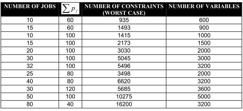
Let us see the effect of number of jobs n and the sum of processing times
å
jpj on the
number of constraints generated by the model.
Assuming the ratio of the number of arcs to number of jobs as 1.5, we can arrive at the following expression:
Number of constraints = 2n2 + 2 T + 1.5n + nT.
where T is the scheduling time horizon. Since, we are illustrating the worst case
scenario, value of T is taken as the maximum possible value
å
jpj. In general, the value of T is very less compared to sum of the processing times. An example is demonstrated in Appendix.C. Thus we can say that the maximum number of constraints are 2n2 + (n+2)å
j pj + 1.5n. The number of variables is nT. Table: 1 gives an idea of the
numbers discussed.
NUMBER OF JOBS
å
j
p NUMBER OF CONSTRAINTS
(WORST CASE) NUMBER OF VARIABLES
10 60 935 600
15 60 1493 900
10 100 1415 1000
15 100 2173 1500
20 100 3030 2000
30 100 5045 3000
32 100 5496 3200
25 80 3498 2000
40 80 6620 3200
30 120 5685 3600
50 100 10275 5000
80 40 16200 3200
Table 1: Computational Complexity of different problems
solved in Lingo is shown in Appendix.C. At this present time and with the computing facilities at out disposal (Industrial LINGO which has a limitation of 16000 constraints and 3200 integer variables.), it is computationally infeasible to attempt to solve large problems by the above integer programming formulation.
Chapter 3
The Approach
The case of a single resource in which the jobs possess series-parallel (s/p) precedence, under the objective of minimizing weighted completion times, has been solved by a procedure by Lawler [6]. For the case of parallel machines with the objective of minimizing the weighted completion time, was solved, using genetic algorithm, by Elmaghraby and Ramachandra [3].
In this chapter, a four-phases, plus an auxiliary phase algorithm is proposed to solve the problem with the objective of minimizing the sum of weighted completion times. The salient feature of this algorithm lies in the packing procedure and the branch and bound procedure, which are to be explained below. Lawler’s algorithm to solve single machine sequencing is shown with an example. Elmaghraby’s procedure [2] to translate the non-s/p graph into s/p graph is also illustrated with some examples.
3.1
Phases in the Proposed Algorithm:
The approach to the solution of this problem is composed of four phases, plus an auxiliary phase, which are briefly explained below.
minimal number of a.p.r.’s, and the procedure is illustrated in Appendix.A to find the a.p.r’s to be added.
• The second phase optimizes the sequence assuming that all jobs require all the resources simultaneously. This is accomplished using Lawler’s [6] procedure.
• The third phase ‘packs’ the solution secured by this optimization to take advantage of the resource options (namely, the fact that some jobs require only a subset of the resources for their accomplishment).
• The fourth phase searches for the optimum by reversing a subset of the a.p.r.’s and repeating the previous three phases. Upon completion of all such reversals, the best sequence is selected. For the sake of brevity we refer to a reversed a.p.r., or a subset of the a.p.r.’s, as ‘ r-a.p.r.’.
It is easily seen that the computational difficulty stems from the enumeration over the subsets of a.p.r. reversals, which is of O(2m), where ‘m’ is the number of a.p.r.’s
introduced. This explains our suggestion on seeking the minimal number of a.p.r.’s. We therefore offer, as a fifth and complementary phase,
3.2. Premises of the Proposed Algorithm
The validity of the proposed procedure rests on the following premises. The demonstration of the validity of the various assertions (except the ‘packing’ procedure) is given in Elmaghraby [2].
1. The optimum occurs at an ‘extreme point’, which is defined as a graph composed of the o.p.r.’s and a set of a.p.r.’s and r-a.p.r.’s that render the graph s/p.
2. It is possible to transform a non-s/p graph into a s/p graph in polynomial time.
3. It is possible to determine the optimal sequence of a set of jobs with s/p
precedence over m different resources (each of unit availability) in polynomial time. This is achieved by applying Lawler’s algorithm followed by a ‘packing’ step.
4. The reversal of any a.p.r., or a subset of the a.p.r.’s, may result in a s/p graph, at which time its optimal schedule is evaluated as in 3. In case the reversal of the subset of a.p.r.’s does not result in a s/p graph2, additional a.p.r.’s are added to render the graph s/p under the specified reversal. This gives rise to a set of subsidiary optimization problems, usually of a much smaller size than the original problem. The subsidiary optimization problems are evaluated by evaluating their optimal solutions. The best result is retained as the optimum under the specified original reversal, together with its ‘auxiliary’ a.p.r.’s, if any are present in the optimum.
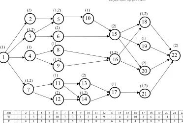
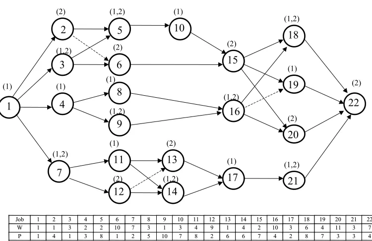
We illustrate the transformation from a non-s/p graph into a s/p by exhibiting the a.p.r.’s for the jobs of Fig.1, with all redundant arcs (due to transitivity) deleted. Observe that Fig.2 contains 3 a.p.r.’s; viz., (2,6), (12,13), and (16,19).
An iteration coincides with the reversal of a subset of the a.p.r.’s. At each iteration all redundant o.p.r.’s in the previous iteration must be re-instituted because the reversed set of a.p.r.’s may result in a different set of redundant o.p.r.’s, or even redundant a.p.r.’s. These redundant arcs are deleted before continuing with the optimization procedure at this iteration.
The optimum for this set of a.p.r.’s, assuming that all jobs require both resources (and hence not taking advantage of the possibility of parallel processing on the two resources) is as follows:
S (0) = {1, 7, 12, 3, 2, 6, 4, 8, 9, 16, 5, 10, 15, 20, 18, 11, 14, 13, 17, 21, 19, 22}; (3.1)
v (0) = 4364. (3.2)
2 This occurs whenever the presence of the a.p.r.’s causes some of the o.p.r.’s to become redundant in the
22 1 13 10 17 16 15 21 20 19 18 9 8 14 12 11 (2) (1) (1,2) (1) (1,2) (1,2) (2) (1) (1,2) (1) (2) (1,2) (1) (2) (2) (1,2) (1,2) (1,2) (1) (2) (1) (2) 2 3 4 5 6 7
22 job non-s/p problem
J
Joobb 11 22 33 44 55 66 77 88 99 1100 1111 1122 1133 1144 1155 1166 1177 1188 1199 2200 2211 2222
W
W 11 11 33 22 22 1100 77 33 11 33 44 99 11 44 22 1100 33 66 44 1111 33 77
P
P 11 44 11 33 88 11 22 55 1100 77 88 22 66 66 77 44 22 88 77 33 33 44
22 1 13 10 17 16 15 21 20 19 18 9 8 14 12 11 (2) (1) (1,2) (1) (1,2) (1,2) (2) (1) (1,2) (1) (2) (1,2) (1) (2) (2) (1,2) (1,2) (1,2) (1) (2) (1) (2) 2 3 4 5 6 7
22 job problem with added apr’s.
J
Joobb 11 22 33 44 55 66 77 88 99 1100 1111 1122 1133 1144 1155 1166 1177 1188 1199 2200 2211 2222
W
W 11 11 33 22 22 1100 77 33 11 33 44 99 11 44 22 1100 33 66 44 1111 33 77
P
P 11 44 11 33 88 11 22 55 1100 77 88 22 66 66 77 44 22 88 77 33 33 44
3.3.
Some Definitions
In this section we discuss the important terms which are used in the rest of the chapters. The terms to be introduced are series-parallel graph (s/p) and interdictive graph (IG).
3.3.1
Series – Parallel graph
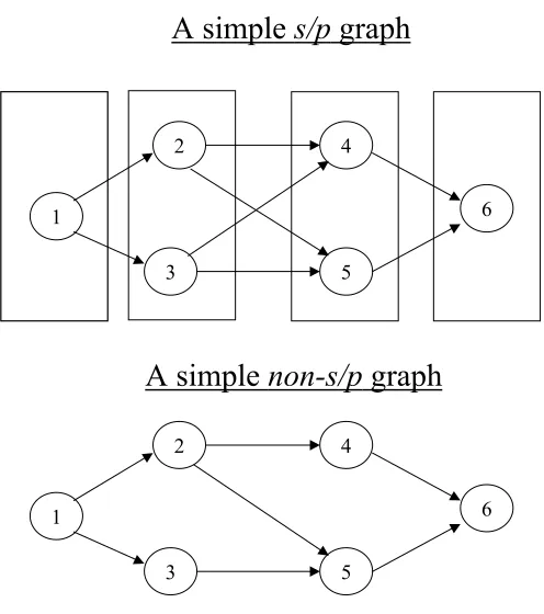
A series-parallel (s/p) graph is defined in different ways in the literature. A simple s/p graph is shown in Figure: 1 and it is compared with a non-s/p graph in the same figure. It can be seen that the s/p graph is divided into four blocks. Every job in a block precedes every job in the succeeding block. For example, every job in block containing {4,5} succeeds every job in block containing {2,3}. It can be compared with a simple non-s/p graph where this condition does not hold true. The recognition of the s/p graph is clearly explained by Valdes et al [12].
3.3.2
Interdictive Graph
1
2
6
3 5
4
1
2
6
3 5
4
A simple
s/p
graph
A simple
non-s/p
graph
1
2
3
4
(a) The IG (JoN)
1
2
3
4
(c) Completing the s/p
by
a.p.r
(1,4)
1
2
3
4
(e) Completing the s/p
by
a.p.r
(2,1)
1
2
3
4
(d) Completing the s/p
by
a.p.r
(4,3)
p
r
q
s
(b) IG (JoA mode)
1
2
3
4
Cross-Arc
3.4.
The Algorithm
The various phases in the proposed algorithm are explained in detail in the following pages.
3.4.1
Transformation of non-s/p graph into a s/p graph
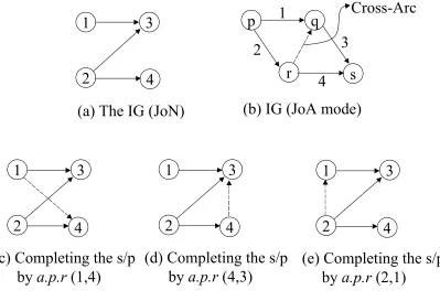
Since the fundamental building block of non-s/p graphs is the so-called ‘interdictive graph’ (IG), it is sufficient to find the a.p.r’s such that these IG’s are removed. Consider four jobs 1,2,3,4 that are related by the precedence relations depicted in Fig.4(a). The graph also shows various methods of converting the graph into a s/p
graph. It can be seen that for a simple graph like Fig.4.a, we have three different possibilities. As the number of the interdictive graphs that are embedded in a graph increases, the problem of finding a minimal number of a.p.r’s needed to transform into a
s/p, becomes complicated. An O(n2.5) algorithm for the minimal node reduction is given by Bein et al [1]. This is an important observation because for the NP-hard problems, we can find algorithms that are exponential only in the minimal number of node reductions rather than the number of vertices. This algorithm has been improved by Elmaghraby [2], to find the number of a.p.r’s for a large problem and is given in App.A. Achieving the minimum number of a.p.r’s in the transformation is desirable but not essential because of the subsequent reversals of all subsets of the a.p.r’s. Excess a.p.r’s at the outset will take its toll in increased number of reversed subsets. This, however, may be mitigated by improved bounds.
3.4.2
Optimal Sequence for single machine problem–Lawler’s
procedure
This algorithm starts with the construction of the decomposition tree of the
series-parallel graph. Proceed from the bottom of the decomposition tree upward, finding an optimal sequence for a module M from previously determined optimal sequences for its sons, M1 and M2. We define ρ(i) = w(i) / p(i), for every job i.
For the parallel composition of M1 and M2, all that is necessary is to form the
union of the two sets M1 and M2. Nonincreasing w/p ratio order is feasible and optimal for
M = M1 ∪ M2, assuming this is true for M1, M2 individually.
For series composition of M1 and M2, the procedure is outlined below. In order
to avoid tests for emptiness, it is assumed that M1 contains a dummy element with ratio
+∝ and M2 a dummy element with ratio –∝. Also, note that at each step, the modules M1
and M2 are to be updated based on some rules (explained below).
Step.1. Find a minimal element ‘ i ’ in M1 and a maximal element j in M2. If ρ(i)
> ρ(j), let M= M1 ∪ M2 and halt. Otherwise, remove i from M1, j from M2 and
form the composite job k = (i,j). Note that the minimal element in any module is defined as the element that has the minimum ratio of w/p.
Similarly, the maximal element in any module is defined as the element that has the maximum ratio of w/p. These elements, themselves, can be a set of jobs.
Step.2.
2.1. Find a minimal element i in M1. If ρ(i) > ρ(k), go to Step 3.1.
2.1. Remove i from M1 and form new composite job k=(i,k). Return to Step 2.1
Step.3.
3.1. Find a maximal element j in M2. If ρ(k) > ρ(j), let M= M1 ∪ M2 ∪ {k} and
An example with 22 jobs (Figure:2) is considered to illustrate the Lawler’s procedure.
4 8 9 16 2 3 5 10 6 15 18 19 7 12 14 17
20
13 11
P1 S2
S3
S5 S8
P4
S7
P10 P6
P9
21 P11
22
P13 S15
P14 P19
S12
S18
S17 S16
S21
1 S20
Consider the digraph G1 with 22 jobs in Figure:2 with the weights and the
processing times (shown in the diagram itself). Assume that all the jobs need all the resources at the same time. Optimal solutions for the various sub-problems, defined by the decomposition tree in Figure:5 are as follows. We denote the composite jobs by sequences, e.g. M7 contains the elementary jobs 6, 15 and a composite job (5,10). The
weights and processing times and the ratios of w/p before and after the Lawler’s algorithm is applied are shown in the table 2.
P1: M1={8,9},
S2: M2={4,8,9},
S3: M3={(4,8,9,16)},
P4: M4={3,2},
S5: M5={(5,10)},
P6: M6={6,(5,10)},
S7: M7={6,(5,10),15},
S8: M8={3,(2,6),(5,10),15},
P9: M9={3,(2,6),(4,8,9,16),(5,10),15},
P10: M10={18,19},
P11: M11={20,18,19},
S12: M12={3,(2,6),(4,8,9,16),(5,10,15,20,18),19},
P13: M13={12,11},
P14: M14={14,13},
S15: M15={12,(11,14),13},
S16: M16={(7,12),(11,14),13},
S17: M17={17,21},
S18: M18={(7,12),(11,14,13,17,21)},
P19: M19={(7,12),3,(2,6),(4,8,9,16),(5,10,15,20,18), (11,14,13,17,21),19},
S20: M20={(7,12),3,(2,6),(4,8,9,16),(5,10,15,20,18), (11,14,13,17,21,19,22)},
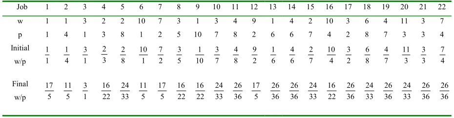
Job 1 2 3 4 5 6 7 8 9 10 11 12 13 14 15 16 17 18 19 20 21 22 w 1 1 3 2 2 10 7 3 1 3 4 9 1 4 2 10 3 6 4 11 3 7 p 1 4 1 3 8 1 2 5 10 7 8 2 6 6 7 4 2 8 7 3 3 4 Initial w/p 1 1 4 1 1 3 3 2 8 2 1 10 2 7 5 3 10 1 7 3 8 4 2 9 6 1 6 4 7 2 4 10 2 3 8 6 7 4 3 11 3 3 4 7 Final w/p 5 17 5 11 1 3 22 16 33 24 5 11 5 17 22 16 22 16 33 24 36 26 5 17 36 26 36 26 33 24 22 16 36 26 33 24 36 26 33 24 36 26 36 26
Table 2: Initial and Final values of w/p ratio
The sequence at the end of the iterations is denoted by S21. This is the optimal
sequence for the problem considered. Note that all these modules (set of node(s)) are in the non-increasing order of ‘w/p’ ratio.
3.4.3
The ‘Packing’ Procedure
At each iteration the packing procedure is initiated with the optimal sequence of the jobs under the specified precedence relations (composed of non-redundant o.p.r.’s,
a.p.r.’s, and any r-a.p.r.’s) assuming that each job requires all the resources for its accomplishment. We refer to such sequence generically as S(0) = (i1, · · · , in) , in which
the subscript identifies the position of the job in the sequence. An example is given in eq.(3.1) in which i1 = 1, i2 = 7, i3 = 12, i4 = 3; etc. Sequence S(0) does not take advantage
of the possibility of processing the jobs in parallel if they demand different resources, and therefore yields an upper bound on the optimum. Indeed, if the first M jobs in the sequence S(0) are mutually independent and require different resources, then it is possible to advance the initiation of their processing to time 0 with considerable gain in the objective function. This observation is the key to the packing procedure.
The packing procedure considers the jobs sequentially in the order of their presence in S0, advancing job ir to the earliest position consistent with the precedence
Proposition 1: The packing procedure results in the optimal sequence under the specified o.p.r.’s.
Proof. In the sequence S(0) job is, s = 2, · · · , n , cannot precede job ir for any r < s, if
the two jobs are related by precedence so that ir p is. Therefore, the only possibility of
having is preceding ir if they require different resources and are not related by precedence, in which case it advances as much as it is resource and sequence feasible. This is precisely what the packing procedure accomplishes.
Optimality results from the fact that the sequence S(0) is optimal in the more restricted subspace of feasible sequences. Call it Ω0. Identify the space of feasible
sequences relative to resource set k by Ωk.3 Clearly, Ω∪Ωk≡Ω0⊂Ω∪Ωk, k = 1, · · · ,2m - 1.
The packing procedure achieves the maximal relaxation of S(0), subject to the ordering imposed by S (0), that is consistent with all other constraints. Hence it is optimal.4
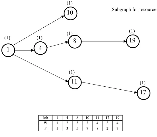
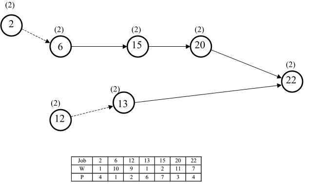
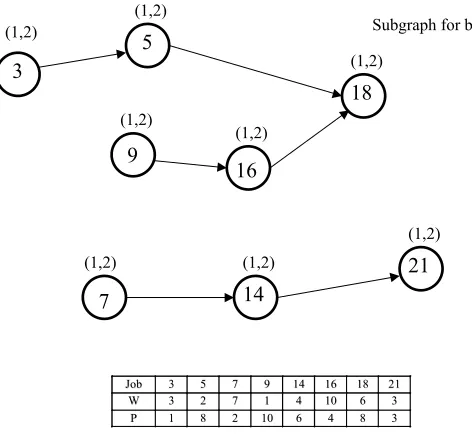
In the illustrative example of Fig.2 there are three possible combinations of resources, viz., a job may require resource 1, or resource 2, or both resources 1and 2, each resulting in a separate subgraph. We illustrate these subgraphs in Figs.6-8. (In these graphs all redundant relations have been deleted.) The sequence is compared with the actual sequence S(0), given in (3.1).
The optimal sequence obtained from the Lawler’s algorithm (phase 2) along with the starting times of the jobs is shown in the Table.3. These values of the start times do not include the ‘packing’ procedure.
J
Joobb 11 44 88 1100 1111 1177 1199
W
W 11 22 33 33 44 33 44 P
P 11 33 55 77 88 22 77
1
10
17 19 8
11
(1) (1) (1)
(1) (1)
(1)
(1) 4
Subgraph for resource 1
J
Joobb 22 66 1122 1133 1155 2200 2222 W
W 11 1100 99 11 22 1111 77
P
P 44 11 22 66 77 33 44
2 (2)
13 (2)
12 (2)
15 (2)
20 (2)
22 (2) (2)
6
Subgraph for resource 2
3 (1,2)
16 (1,2)
7 (1,2)
5 (1,2)
18 (1,2)
14 (1,2) (1,2)
9
Subgraph for both resources 1 & 2
J
Joobb 33 55 77 99 1144 1166 1188 2211 W
W 33 22 77 11 44 1100 66 33
P
P 11 88 22 1100 66 44 88 33
21 (1,2)
Job 1 7 12 3 2 6 4 8 9 16 5 10 15 20 18 11 14 13 17 21 19 22
Start Time 0 1 3 5 6 10 11 14 19 29 33 41 48 55 58 66 74 80 86 88 91 98
Table 3: Start Times for 22 jobs in the optimal sequence
Value of the ‘raw’ sequence v(0) = 4364.
The optimal sequences for the three resources individually are as follows:
S (1) = (1, 11, 17, 4, 8, 9, 10) (3.3) S (2) = (12, 2, 6, 15, 20, 13, 22) (3.4) S (1, 2) = (7, 3, 14, 21, 9, 16, 18, 5) (3.5)
The ‘packed sequence’ is easily derived from S(0) and is shown in Table:4 (jobs marked in bold demand both resources):
Resource 1: 1 7 3 4 8 9 16 5 10 18 11 14 17 21 19
Resource 2: 7 12 3 2 6 9 16 5 15 20 18 14 13 21 22 9
Start Time: 0 1 3 5 6 10
14 24 28 36 43 50 53 61 69 75 81 83 86 93
Table 4: Start Times of 22 jobs after the ‘packing’ procedure
Value of packed sequence v* (0) = 4034.
gained in value by processing jobs 4,8 in parallel with 2,6. The starting time of the job 9 is at time t = 14. This is secured by the maximum of {s(4)+p(4)+p(8) , s(2)+p(2)+p(6)}, where s(i) and p(i) are the starting time and processing time of job ‘i’ respectively. The packed sequence deviates from either S(1) and/or S(2) when the jobs in either sequence
are unrelated. For instance, S(1) specifies that 17 p 4, while the optimal sequence
reverses the order. To be sure, jobs 4 and 17 are unrelated (see Fig.6); etc. This is demonstrated because the efforts to find the individual sequences and then merging them to get the final optimal sequence were futile and this approach can be ignored for further research. Another method which was futile is the decomposition of original s/p graph into ‘r’ subgraphs (note that r refers to number of resources) and then finding the optimal sequence for each of the graphs. This method can also be ignored for further research as this will not take into account some of the precedence relations which were present in the original graph and are not reflected when split into subgraphs.
3.4.4
Optimal Sequence – An approach by optimization via the
reversal of
a.p.r’s
The optimal sequence is found by enumerating all the possible subsets of the
a.p.r reversals. All possible reversals are to be considered due to the fact that we are adding some of the additional precedence relations between the nodes which were not related before. The complete enumeration of all possible reversals of the a.p.r.’s, and there are 7 of them in this example of 22 jobs has resulted in the following optima (see Table.5 for the identity of the reversed a.p.r.’s).
We conclude that the optimal sequence is given by the no reversal instance,
S* = the packed sequence without any reversals
3.4.5
Branch and Bound (BaB) procedure
The exponential nature of the search domain for the optimum suggests the use of the BaB approach, in the hope that the overwhelming majority of the feasible sequences would be fathomed implicitly, with evident computing advantages. There are two concerns:
Table 5: Optimal Values and Lower bounds for the enumerated subset of a.p.r reversals
REVERSAL OPTION OPTIMUM VALUE LOWER BOUND
1. Branching. It is evident that the offsprings of any node in the BaB search tree are the possible reversals of the ‘residual’ a.p.r.’s in the graph. The ‘origin’ of the BaB search tree is the complete s/p graph (all a.p.r.’s included). Its immediate descendents are the K possible reversals; each representing the reversal of one
a.p.r. The descendant of each one of these nodes is the K-1 possible reversals of the other a.p.r.’s; etc.
2. Bounding. A fundamental concern in the BaB approach is the development of
‘strong’ lower bounds (l.b.). This concept of bounding is very important, as it is possible to abort the search as soon as we achieve results within a certain specified range of the bounds. The strongest l.b. is secured by determining the
minimum number of o.p.r.’s to delete from the original graph when the subset of
a.p.r.’s are reversed and all other a.p.r.’s are removed.4 (Alternatively, we seek the maximal graph of the o.p.r.’s that is s/p under the specified r-o.p.r.’s.) To clarify this construction, consider the reversal of a.p.r.’s (2,6) and (12,13) in the graph of Fig.2. (This reversal is #4 in Table 5.) Upon deleting the remaining a.p.r.
(specifically, arc (16,19)) the graph would appear as shown in Fig.9. Arcs (1,2),(3,5) and (6,15) become redundant; so do arcs (7,12),(11,14) and (13,17). The simplified (i.e., without the redundant o.p.r.’s) graph is shown in Fig.10. It is evident that removing arc (15,19) rendered the graph s/p.5
The optimal packed sequence of the jobs under the precedence relations of Fig.10 is:
S(0) = (1, 3, 6, 7, 11, 13, 12, 14, 17, 21, 4, 8, 9, 16, 2, 5, 10, 15, 20, 18, 19, 22) v(0) = 4537.
4 Recall that all o.p.r.’s are re-instituted at each iteration.
5 A more formal procedure to identify the maximal reduced graph is described by Elmaghraby[2] and is
22 1 13 10 17 16 15 21 20 19 18 9 8 14 12 11 (2) (1) (1,2) (1) (1,2) (1,2) (2) (1) (1,2) (1) (2) (1,2) (1) (2) (2) (1,2) (1,2) (1,2) (1) (2) (1) (2) 2 3 4 5 6 7 Reverse (2,6)&(12,13) G R R R R J
Joobb 11 22 33 44 55 66 77 88 99 1100 1111 1122 1133 1144 1155 1166 1177 1188 1199 2200 2211 2222 W
W 11 11 33 22 22 1100 77 33 11 33 44 99 11 44 22 1100 33 66 44 1111 33 77
P
P 11 44 11 33 88 11 22 55 1100 77 88 22 66 66 77 44 22 88 77 33 33 44
R
R
Figure 9: Reversing a.p.r’s (2,6) and (12,13).
22 1 13 10 17 16 15 21 20 19 18 9 8 14 12 11 (2) (1) (1,2) (1) (1,2) (1,2) (2) (1) (1,2) (1) (2) (1,2) (1) (2) (2) (1,2) (1,2) (1,2) (1) (2) (1) (2) 2 3 4 5 6 7 Reverse (2,6)&(12,13) and remove redundant opr’s
J
Joobb 11 22 33 44 55 66 77 88 99 1100 1111 1122 1133 1144 1155 1166 1177 1188 1199 2200 2211 2222 W
W 11 11 33 22 22 1100 77 33 11 33 44 99 11 44 22 1100 33 66 44 1111 33 77
P
P 11 44 11 33 88 11 22 55 1100 77 88 22 66 66 77 44 22 88 77 33 33 44
Resource 1: 1 3 7 11 14 17 21 4 8 9 16 5 10 18 19
Resource 2: 3 6 7 13 12 14 21 9 16 2 5 15 20 18 22
-Start Time: 0 1 2 3 5
11
13 19 21 24 27 32 42 46 50 58 65 72 75 83 90
Table 6: Start Times for the optimal sequence of figure 9
Emulating the BaB procedure for this example would result in the search tree exhibited in Fig.11.
Since the parent node has an optimum that is smaller than the l.b. of any of its three descendents, they are fathomed and we declare the sequence given by the packed sequence of eq.(3.1) to be optimal, with value of 4034.
Reverse apr (2,6) Opt= 4129, LB=4123
fathomed
Reverse apr (12,13) Opt=4713, LB=4537
fathomed
Reverse apr (16,19) Opt=4279, LB=4146
fathomed
Completed s/p graph with
apr's (2,6),(12,13),(16,19) Opt=4034,LB=4034
optimal
3.5.
Algorithm – Implementation on a 17- Job problem:
A 17 job problem is given in Fig.12. The proposed algorithm has been implemented on this complex and more general problem. The numbers mentioned over each job represent the resource on which it needs to be processed. The weights and the processing times of each job are also mentioned in the table in the figure.
This problem is more complex in nature when compared to the problem of 22 jobs due to the fact that some of the interdictive graphs are embedded inside the other interdictive graphs. This property will be common to most of the graphs and the problem will become more difficult to solve as the number of embedded interdictive graphs increases.
The original 17 job problem is a non-s/p graph. The number of a.p.r’s is found using an approach mentioned by Elmaghraby. The minimala.p.r’s to be added to make it a s/p graph are (2,3), (5,6), (16,15), (13,15). The s/p graph obtained by incorporating the
a.p.r’s is shown in Fig.13.
This problem is solved for the optimality by the Lawler’s procedure and the sequence obtained is:
S (0) = {(1,2,5,7,3), (8,12), (6,11,16), 4,14,10, (13,9,15,17)}
V (0) = 1805.
(1) 1
(2) 8 (1,2) 6 (1,2)
2
(1) 4 (2)
3
(1,2) 12 (1,2)
7 (1)
9 (2)
5
(1,2) 14
(1) 15
(1,2) 16 (1)
11 (2) 10
(2) 17 (1,2)
13
17 Job problem- Original
J
Joobb 11 22 33 44 55 66 77 88 99 1100 1111 1122 1133 1144 1155 1166 1177
W
W 11 11 33 22 77 22 1100 33 11 33 44 99 11 44 22 1100 33
P
P 11 44 11 33 22 88 11 55 1100 77 88 22 66 66 77 44 22
(1) 1 (2) 8 (1,2) 6 (1,2) 2 (1) 4 (2) 3 (1,2) 12 (1,2) 7 (1) 9 (2) 5 (1,2) 14 (1) 15 (1,2) 16 (1) 11 (2) 10 (2) 17 (1,2) 13
R
R
17 Jobs - includinga.p.r’s
J
Joobb 11 22 33 44 55 66 77 88 99 1100 1111 1122 1133 1144 1155 1166 1177
W
W 11 11 33 22 77 22 1100 33 11 33 44 99 11 44 22 1100 33
P
P 11 44 11 33 22 88 11 55 1100 77 88 22 66 66 77 44 22
R
R
In the fourth stage, a subset of the a.p.r’s is reversed and is checked for the optimality by repeating the above three phases. Upon completion of the all such reversals, the best sequence is selected. An example when the a.p.r (5,6) is reversed is in Fig. 13. It is required that an auxiliary a.p.r (6,2) must be added to make the graph a s/p
graph. Also note that this makes the r-a.p.r (5,6) redundant. The s/p graph obtained by this conversion is shown in Fig.14. Another example where the a.p.r (16,15) is reversed is also illustrated in the Fig.15. For this graph to be turned into a s/p graph, we need to add an auxiliary a.p.r (11,15). The s/p graph obtained without the redundant arcs is shown in Fig.16.
The branch-and-bound procedure that enumerates the possible alternatives is performed. The details of the iterations, the o.p.r’s to be removed at each iteration (for the calculation of the lower bounds), and the redundant arcs are shown in Table.7. The optimal values and the lower bounds are calculated at each iteration and are listed in Table. 8.
The optimal sequence has a minimum value of 1752 for iteration # 6. This is achieved by r-a.p.r (2,3) and r-a.p.r (13,15). The corresponding optimal sequence is:
S*(Opt) = {1,3,2,5,7,8,12,6,11,16,4,14,10,9,15,13,17}
V*(Opt) = 1752.
The BaB tree is shown in the Fig.17. The braches of the tree will get fathomed because their values of the lower bounds are greater than the optimal value (1752) found. The BaB tree shows that it is not necessary to enumerate all the (2m-1) subsets of reversals. This BaB procedure gives an option to stop the iterations when the bound deviates from the optimal value by a certain known amount. It emulates the process in case of large problems. Indeed, if we stop after the first range of descendents, we would have obtained a feasible schedule of value 1755, and the smallest lower bound is 1752.
So one can stop with maximum error of 0.17% 1752
1752 1755
= −
J
Joobb 11 22 33 44 55 66 77 88 99 1100 1111 1122 1133 1144 1155 1166 1177
W
W 11 11 33 22 77 22 1100 33 11 33 44 99 11 44 22 1100 33
P
P 11 44 11 33 22 88 11 55 1100 77 88 22 66 66 77 44 22
(1) 1 (2) 8 (1,2) 6 (1,2) 2 (1) 4 (2) 3 (1,2) 12 (1,2) 7 (1) 9 (2) 5 (1,2) 14 (1) 15 (1,2) 16 (1) 11 (2) 10 (2) 17 (1,2) 13
R
R
Reverse (5,6) Add auxiliary apr (6,2)R
R
R
R
R
J
Joobb 11 22 33 44 55 66 77 88 99 1100 1111 1122 1133 1144 1155 1166 1177
W
W 11 11 33 22 77 22 1100 33 11 33 44 99 11 44 22 1100 33
P
P 11 44 11 33 22 88 11 55 1100 77 88 22 66 66 77 44 22
(1) 1 (2) 8 (1,2) 6 (1,2) 2 (1) 4 (2) 3 (1,2) 12 (1,2) 7 (1) 9 (2) 5 (1,2) 14 (1) 15 (1,2) 16 (1) 11 (2) 10 (2) 17 (1,2) 13 Reverse (5,6) Add auxiliary apr (6,2)
Remove redundant arcs
J
Joobb 11 22 33 44 55 66 77 88 99 1100 1111 1122 1133 1144 1155 1166 1177 W
W 11 11 33 22 77 22 1100 33 11 33 44 99 11 44 22 1100 33
P
P 11 44 11 33 22 88 11 55 1100 77 88 22 66 66 77 44 22
(1) 1 (2) 8 (1,2) 6 (1,2) 2 (1) 4 (2) 3 (1,2) 12 (1,2) 7 (1) 9 (2) 5 (1,2) 14 (1) 15 (1,2) 16 (1) 11 (2) 10 (2) 17 (1,2) 13
R
R
Reverse (16,15) Add auxiliary apr (11,15)R
R
R
J
Joobb 11 22 33 44 55 66 77 88 99 1100 1111 1122 1133 1144 1155 1166 1177 W
W 11 11 33 22 77 22 1100 33 11 33 44 99 11 44 22 1100 33
P
P 11 44 11 33 22 88 11 55 1100 77 88 22 66 66 77 44 22
(1) 1 (2) 8 (1,2) 6 (1,2) 2 (1) 4 (2) 3 (1,2) 12 (1,2) 7 (1) 9 (2) 5 (1,2) 14 (1) 15 (1,2) 16 (1) 11 (2) 10 (2) 17 (1,2) 13 Reverse (16,15) Add auxiliary apr (11,15)
Remove redundant arcs
Table. 7: Details of the “OPRs to be removed to render s/p” for the 17 job problem.
# Arcs Reversed/Added OPRs to be removed Redundant Arcs
0 None ---
---1 (2,3) (6,10), (7,11), (5,13) (1,2),(3,14)
2 (5,6) Add(6,2) (3,14), (7,11), (5,13), (1,3) (1,2),(6,5),(6,10),(6,11) 3 (13,15) (6,10), (7,11), (3,14) (5,13),(15,17)
4 (16,15) Add(11,15) (6,10), (7,11), (3,14), (5,13), (1,3)
(11,16),(15,17)
5 (2,3), (5,6) Add(6,2) (7,11), (5,13), (6,11) (1,2),(3,14),(6,5),(6,10) 6 (2,3), (13,15) (6,10), (7,11) (1,2),(3,14),(15,17),(5,13) 7 (2,3), (16,15) Add(11,15) (6,10),(7,11),(5,13) (1,2),(3,14), (11,16),(15,17) 8 (13,15),(5,6) Add(6,2), (7,11),(3,14),(1,3) (5,13),(15,17), (1,2),(6,5), (6,10),
(6,11) 9 (5,6),(16,15),Add(6,2),
Add(11,15)
(3,14),(5,13),(11,15) (1,2),(6,5),(6,10),(6,11),(11,16), (15,17)
10 (13,15),(16,15) Add(11,15) (6,10),(7,11),(3,14),(1,3) (5,13),(11,16),(15,17) 11 (2,3),(5,6),(13,15),Add(6,2
)
(7,11) (1,2),(3,14),(6,5),(6,10), (6,11), (5,13),(15,17)
12 (2,3),(5,6),(16,15),Add (6,2), Add(11,15)
(5,13),(11,15),(6,11),(11,16 )
(1,2),(3,14),(6,5),(6,10),(15,17)
13 (2,3),(13,15),(16,15), Add(11,15)
(6,10),(7,11) (1,2),(3,14),(5,13),(15,17),(11,16)
14 (13,15),(5,6),(16,15),Add (6,2), Add(11,15)
(3,14),(6,11),(11,16) (1,2),(6,5),(6,10),(5,13),(15,17)
15 (2,3),(13,15),(5,6),(16,15), Add (6,2), Add(11,15)
Table.8: The optimal and the Lower bounds of various iterations (17 jobs)
# Arcs Reversed/Added Optimal Value Lower Bound
0 No reversal 1805 1805
1 (2,3) 1802 1752
2 (5,6) Add(6,2) 1978 1889
3 (13,15) 1755 1752
4 (16,15) Add(11,15) 1958 1833
5 (2,3), (5,6) Add(6,2) 1974 1924
6 (2,3), (13,15) 1752 1752
7 (2,3), (16,15) Add(11,15) 1955 1898
8 (13,15),(5,6) Add(6,2), 1928 1889
9 (5,6),(16,15),Add(6,2), Add(11,15) 2161 2007
10 (13,15),(16,15) Add(11,15) 1901 1833
11 (2,3),(5,6),(13,15),Add(6,2) 1924 1924
12 (2,3),(5,6),(16,15),Add (6,2), Add(11,15) 2157 2072 13 (2,3),(13,15),(16,15),Add(11,15) 1898 1898 14 (13,15),(5,6),(16,15),Add (6,2), Add(11,15) 2104 2035 15 (2,3),(13,15),(5,6),(16,15), Add (6,2),
Add(11,15)
Reverse (2,3) Opt=1802,LB=1752
fathomed
Reverse (5,6) Add(6,2) Opt=1978,LB=1889
fathomed
Reverse (2,3) Opt=1752,LB=1752
Optimal
Reverse (5,6) Add(6,2) Opt=1928,LB=1889
fathomed
Reverse (16,15) Add(11,15) Opt=1901,LB=1833
fathomed
Reverse (13,15) Opt=1755,LB=1752
Reverse (16,15) Add(11,15) Opt=1958,LB=1833
fathomed
Completed s/p graph with aprs (2,3), (5,6),(13,15),(16,15)
Opt=1805,LB=1805
Figure 18: BaB tree for the 17 job problem
Chapter 4
Conclusions and Future Research
4.1.
Conclusions
In this thesis, the difficult problem of scheduling precedence-related jobs on R processors/resources with the objective of minimizing the sum of the weighted completion times was addressed. First, we proposed a binary integer program to solve this problem. This formulated using LINGO. The total number of constraints and variables are functions of the number of jobs and the planning horizon. Given the fact that LINGO is restricted only to 16000 constraints and 3200 integer variables, it is difficult to solve for the larger problems and the algorithms to achieve good results need to be proposed.
An algorithm with 4 phases plus an auxiliary phase is proposed. Lawler’s procedure and Elmaghraby’s procedure to transform non-s/p graph to a s/p graph are explained with two examples. Our approach to the treatment of the P2| prec | åwjCj scheduling problem has been programmed in Matlab for ‘proof of concept’ rather than industrial application. Information regarding the various program files are given in
App.B. The examples treated here were expressly chosen to be simple in order not to obscure the main points of the approach; they are directly applicable to more resources (we have treated only two resources) and to more complex6 precedence graphs.
First, we have treated a rather simple graph adapted from Lawler [6], at the cost of increased computational effort, naturally. In this graph, the a.p.r.’s do not cause
6 The ‘complexity’ of a graph is measured by the number of nodes (jobs), the average order of a node, and
any o.p.r.’s to become redundant. As a consequence, the reversal of any a.p.r (or a subset thereof) shall give rise to a s/p graph. This happy situation may not materialize when an
a.p.r. causes some o.p.r.’s to become redundant. In this case one would be forced to introduce additional a.p.r.(s) to render the graph s/p. The resulting ‘sub-problem’ will have to be resolved before the return to the main problem. This can be demanding computationally, and this is where the BaB approach shines. This special case problem is dealt with a problem of 17 jobs and the results are shown in Tables 7 and 8. BaB approach is very useful in the regard that the algorithm can be terminated as soon as a value is achieved within estimated error in bound.
4.2
.
Future Research Directions
References
1. Bein, W.W., Karburowski, J. and Stallmann, M.F.M. (1992). “Optimal reduction of two-terminal directed acyclic graphs,” SIAM J. Computing 21, 1112-1129.
2. Elmaghraby, S.E. (2001). “On the sequencing of jobs on a single machine to minimize total weighted completion time subject to arbitrary precedence constraints”. In a paper presented at the IETM conference, Quebec City, Canada, August 21-24, 2001.
3. Elmaghraby, S.E. and Ramachandra, G. (2002). “The scheduling of precedence-related jobs on parallel machines,” Tech. Report, North Carolina State University, Raleigh, NC. (to be appeared in Extended Abstract form in the Proc. Of ISS,
Hamanako, Japan, June 4-6, 2002.)
4. Garey, M.R, Johnson, D.S., and Stockmeyer, R.L. (1976). “Some simplified NP-complete graph problems,” Theor. Comp. Sci. 1: 237-267.
5. Klein, R. (2000). “ Scheduling of Resource Constrained Projects”,Kluwer Academic Publishers, Boston.
6. Lawler, E.L. (1978). “Sequencing jobs to minimize total weighted completion time subject to precedence constraints,” Ann. Discr. Math. 2:75-90.
7. Pinedo, Michael. (2002).“Scheduling: Theory, Algorithms and Systems, 2/e”. Prentice Hall.
9. Sidney, J.B. and Steiner, G. (1986). “Optimal sequencing by modular decomposition: Polynomial algorithms,” Oper. Res. 34: 606-612.
10.Smith, W.E. (1956). “Various optimizers for single stage production,” Nav. Res. Log. Quarterly 3: 59-66.
11.Syslo, M.M. (1981). “Optimal constructions of event-node networks,” RAIRO Tech. Oper. 15, 241-260.
12.Valdes, J., Tarjan, R.E and Lawler, E.L.(1982). “The recognition of series-parallel digraphs,” SIAM J. Comp, 11: 298-313, 1982.
Appendix A
The Procedure for finding a.p.r.’s
In this appendix, the steps to construct the a.p.r’s are illustrated.
1. Determine the job-on-node (JoN) graph representing the precedence relations. Call it G.
(a) Check if G is s/p following Valdes, Tarjan and Lawler [12]. If yes, stop; no
a.p.r.’s are needed.
(b) Else, check for G being a line digraph, following Syslo [11]. If yes, go to step 2; else, introduce a minimal number of dummy jobs (also following Syslo) to render it line digraph. (Otherwise dummy arcs shall be needed to accomplish step 2 next.) The augmented graph G is the one used in the sequel.
2. Translate the graph G into a job-on-arc (JoA) graph. Call the resulting graph H. Note that since G is a line digraph there shall be no need for any dummy arcs in H.
3. Determine the dominator tree (DT), the reverse dominator tree (RDT), and the complexity graph (CG) of H following Bein, Kamburowski and Stallmann [1]. Determine the minimum node cover of the CG, and denote it by R. By construction, each node j . R together with each of the arcs incident on it define the ‘cross arc’ (written as “x-arc”) in some interdicting graph (IG) within the original graph G. Denote the set of x-arcs by XA. For each arc in the set XA determine the nearest predecessor and the nearest successor of its terminal nodes in H. Isolate the subgraph of H composed of the union of the nodes in R, their predecessors and successors, and the arcs joining them. Denote the resultant graph by RH for “relevant graph H”. Observe that the graph G as well as the graph RH change as a.p.r.’s are added (due to
4. Let x(i,j) denote cross-arc (i,j ). For each x(i,j ) determine its IG in RH. Let the IG be defined by the four nodes o,i,j,t.
(a) If the path from i to j contains another x-arc, skip this x(i,j ) and proceed with the
IG identified by the x-arc in the path.
(b) Else add the a.p.r. required to ‘dissolve’ the IG7. Incidentally, if all the x-arcs are mutually independent then the resulting a.p.r.’s are minimal, and the reversal of any subset of them defines a s/p graph. This would greatly simplify the evaluation of the reversed a.p.r.’s.
5. When all the x-arcs in this iteration of RH have been scanned,
a) if any x-arcs have been skipped in step 4a, return to step 3 with the added
a.p.r.’s and the modified G.
b) Otherwise, stop. The added a.p.r.’s are suffcient to render the graph G s/p.
Appendix B
Guide to
Matlab
Programs
In this appendix, the Matlab program used is shown. The program contains various sub-programs. Only the outline of the important programs have been shown:
The programs used and the notation followed for the code is as follows:
Notation used:
A- Main matrix (if an arc exists between node 1 and 2 then A (1,2)=1)
Wt- weight array
PT- processing time array
Arcs- a.p.r’s to be added to make the graph s/p
Opr- o.p.r’s to be deleted to calculate the lower bound at each iteration
Ratio- ratio of the weight and processing time
NodeSet1- set of jobs which are to be processed on resource1
NodeSet2- set of jobs which are to be processed on resource2
JoinPS- the set of series/parallels jobs found at the iteration
Trans- transitive matrix of the present A matrix
CombinedNodeSets- module sets that can be found independently from the decomposition tree. These sets needs to merged to get the FinalSequence.
Programs needed to run the code written are as follows:
AssignIndex: assigns the new indices based on the node added.(used for finding internal variables)
AttachIntoFinalSequence: this function attaches the node sets into the final sequence based on the ratio values.
Input: present final sequence, ratio, wt, PT Output: updated final sequence, ratio, wt, PT
AttachNewNodes: this function attaches the newly found related nodes in to the CombindedNodeSets.
Input: ratio, wt, PT, CombinedNodeSets and some internal variables. Output: ratio, wt, PT, CombinedNodeSets
CompletionTimeVersion2: This evaluates the optimal sequence and wct at each iteration.
Input: A, wt, PT, IsItLB
Output: Optimal Sequence, wct
FindParallel: finds whether a parallel relation exists between two nodes or not.
Input: row and column values from transitive matrix for the nodes, which are to be tested for the parallel relation
Output: 1,if the relation is parallel
FindSeries: finds whether a series relation exists between two nodes or not.
Input: row and column values from transitive matrix for the nodes which are to be tested for the series relation
FindSPlinks: finds the nodes which are related (series/parallel)
Input: A, ratio, trans and some internal variables (to know if they are already been assigned or not)
Output: JoinPS
InsertIntoRow: allocates a newly found related node into the row where it is related. i.e., if we find that node 4 is related to [3 2] with series condition then output is [3 2 4].
Input: set of rows, ratio, node to be added
Output: set of rows after the new node is inserted
MainProgramAlgo2Jobs22LB: This is the heart of all the programs and is linked to various other programs.
Input: A, wt, PT, IsItLB Output: FinalSequence
ModifyA: Updates the matrices A and transitive matrices by removing the nodes which were attached into the sequence.
Input: A, JoinPS, trans Output: A,trans
OrderedNode: changes rows of a matrix to the cell array i.e.,[2 3;3 4] is changed to [{2 3}; {3 4}]
Input: any matrix that needs to be changed to cell array Output: cell array of the matrix
Reversals: This is the main program. Input: A, wt, PT, Arcs, Opr
Output: Optimal Sequence, weighted completion time(wct) corresponding to the sequence
Transitive: Finds the transitive of the present A matrix. Input: A
Output: trans
UpdateRatio: this is used to update the values of the ratio, wt, PT while finding the CombinedNodeSets. This is used only for a particular set of nodes.
Input: ratio, wt, PT, node sets for which the values are to be updated Output: ratio, wt, PT ( all are modified)
UpdateRatioInFS: this is also used as in the above with some adjustments so that the final sequence is also taken into account. This is used for variety sets of nodes, which distinguishes this from the above function.