The Interaction Between Moist Convection and African Easterly Waves.

(1)

ABSTRACT

RUSSELL, JAMES OLIVER HARVEY. The Interaction Between Moist Convection and African Easterly Waves. (Under the direction of Anantha Aiyyer).

This dissertation addresses the relationship between African Easterly Waves (AEWs) and moist convection. AEWs are analyzed in two convection-permitting simulations and in composite averages using two reanalyses. This approach allows us to examine the mesoscale characteristics of moist convection while also investigating the synoptic-scale evolution of the AEW. Potential Vorticity (PV) and its budget in various forms, are used extensively to understand the dynamics of the AEWs.

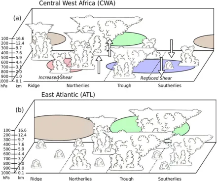
Over land, moist convection is typically in the form of multiple Quasi-Linear Convective Systems (QLCSs) within the northerlies of the wave. Convective initiation in the northerlies occurs through a superposition of the diurnal cycle with AEW-scale forcing for moisture, ascent, and convective inhibition. The resulting QLCSs are enhanced by larger CAPE and a favorable interaction between the enhanced shear and QLCS cold pools. Over ocean, deep moist convection occurs in the trough associated with enhanced moisture and ascent. The coupling of moist convection with the AEW resembles Mapes et al. (2006)stretched building block theory. This manifests in deep moist convection in the northerlies and trailing upper-level stratiform convection in the trough.

(2)

(3)

The Interaction Between Moist Convection and African Easterly Waves

by

James Oliver Harvey Russell

A dissertation submitted to the Graduate Faculty of North Carolina State University

in partial fulfillment of the requirements for the Degree of

Doctor of Philosophy

Marine, Earth, and Atmospheric Sciences

Raleigh, North Carolina 2019

APPROVED BY:

Matthew Parker Gary M. Lackmann

Carl Schreck William Boos

Anantha Aiyyer

(4)

ACKNOWLEDGEMENTS

Thanks first goes to my girlfriend, Gaby, for always being their whenever I needed someone throughout my degree. She has stuck by me all the way, no matter how stressed I was, and despite the sheer amount of time I spent working instead of spending time with her. I would like to thank my family back in England, especially my parents, Barbara and Nigel, for their lifetime of support getting me to this position in my life. I’d also like to thank all my friends, across the world, who have all, at some point supported me, even if it was as small as a quick conversation. My two dogs, Ghost and Ruby, have also helped me through this, simply through fluffy cuddles and always being happy.

I would like to thank my advisor, Dr. Anantha Aiyyer for his support throughout, and all the wisdom he has imparted to me through countless discussions. Special thanks goes to Dylan White for many long discussions, help with code, and moral support throughout my degree. He never failed to be there when I needed someone to discuss anything. Special thanks also goes to Dr. Gary Lackmann for much advice on the use of the WRF model. Thanks also goes to Drs. Matthew Parker, Bill Boos, and Carl Schreck who all provided useful ideas and discussion throughout my degree.

(5)

LIST OF TABLES

Table 2.1 Parameterization schemes used in the 2007 and 2010 simulations. . . 22 Table 2.2 Summary of all simulations. M represents all mixing ratio variables

and MP stands for microphysics. Times are in UTC. . . 25

Table 3.1 Summary of MCSs. L=Land, O=Ocean. Duration is in hours. Speed is in ms−1_{. Direction of motion is given by compass abbreviation (e.g.} westward motion is W). . . 44 Table 3.2 Summary of MCSs relative to AEW. AEW phase is given with the

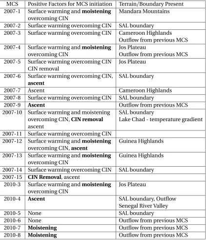
fol-lowing abbreviations; T=Trough, R=Ridge, S=Southerlies, N = Northerlies. Positive zonal motion is faster than the AEW trough (ms−1_). Positive meridional motion is moving northward relative to the AEW (ms−1_{). . . .} ₄₆ Table 3.3 Factors that influenced the initiation of MCSs. Factors in bold are

those supported by the phase of the AEW (e.g. AEW was promoting moistening in area of initiation and moistening also had a role in initiation). . . 63

Table 4.1 Source terms from equation 2.31 contributing to propagation and growth of AEW-scale PV (calculated using equation 4.2) averaged in the volume encompassed by 400–700 hPa, 4–20◦_{N, and 30}◦_W-40◦_E. Anything with a fractional contribution of 0.01 (i.e. 1%) or less was deemed to be negligible and for presentation is represented by a -. . . 89 Table 4.2 Possible interactions between waves in the AEW. PV anomalies are

denoted byP withd for dry waves andm for moist waves, andl o w for

low-level waves and_{m i d} for mid-level waves.Q represents induced diabatic processes enhancing a moist wave andv represents an in-duced cross-advection enhancing a dry wave. PV gradients referred to are those shown in Figure 4.2. . . 95

Table A.1 A summary of acronyms used in alphabetical order. . . 143

(9)

LIST OF FIGURES

Figure 1.1 Time-series (by year) of the a) GF and CF of TCs, b) GF and CF of hurricanes, c) GN and CN of TCs, and d) GN and CN of hurricanes. Red is for GN or GF and blue is for CN and CF. Solid lines indicate time periods surveyed by our study. Dashed lines indicate time periods surveyed by Avila et al. (2000). Horizontal lines represent 1967-2015 averages. . . 3 Figure 1.2 Latitude-height cross-sections of the correlation between GN and

seasonal mean EKE (filled) for a) 30◦_W-30◦_{E, b) 30}◦_{W, c) 15}◦_{W, d) 0}◦_{, e)} 15◦_{E, and f ) 30}◦_{E. Contours represent the seasonal mean EKE (J}_/_kg) and stippling represents statistical significance of 95% for the corre-lations. Outlined areas with numbers represent specific statistically significant areas of correlation discussed in the text. . . 5 Figure 1.3 Janiga and Thorncroft (2016) Figure 17. . . 8 Figure 1.4 A schematic of a DRV in mean westerlies adapted from Parker and

Thorpe (1995). a) depicts a current time and b) depicts a later time. Current positive PV (solid red circles), past positive PV (dashed pink circle), southerlies (X), ascent (w), and diabatic heating (Q) are shown in association with the cloud distribution. . . 10 Figure 1.5 Cohen and Boos (2016) Figure 3. . . 12 Figure 1.6 Vertical cross-sections (x-z) illustrating key properties of the

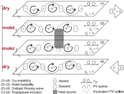
strati-form instability process. . . 13

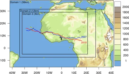
Figure 2.1 WRF domain setup for all simulations with model terrain height (m) shaded. Manually defined AEW tracks following the positive vorticity center and meridional wind minima (i.e. the trough) in the control simulations are shown. The blue track is for the 2007-CTRL AEW (09/06 00Z to 09/17 00Z) and the red track is for the 2010-CTRL AEW (8/19 00Z to 8/27 12Z). . . 21 Figure 2.2 Time-longitude plots of 5-20◦N averaged 650hPa meridional winds

(m/s, filled) and precipitation (mm/hr, only 1mm/hr contour shown) for the a) 2007 AEW in ERAI, b) AEW in 2007-CTRL, c) 2010 AEW in ERAI, and d) AEW in 2010-CTRL. a) and c) use the TRMM 3B42 product to represent precipitation. For comparison all model data is regridded to the ERAI and TRMM grids for winds and precipitation respectively. The analyzed track of the control simulation for each year is represented by the thick green lines. . . 23 Figure 2.3 Wavenumber-frequency power spectrum of the TRMM precipitation

(10)

Figure 2.4 a) and b) variance of 650hPa AEW-scale PV, c) and d) variance of 925hPa AEW-scale PV, e) and f ) average 650hPa AEW-scale EKE, g) and h) average 925hPa AEW-scale EKE. a), c), e), and g) are for ERAI and b), d), f ), and h) are for CFSR. The black line in a) depicts the southern track of AEWs. Black dots and labels indicate composite locations and the names of those locations as referred to in the text. 38 Figure 2.5 Time series of AEW-filtered meridional winds at the base point 10◦N

latitude, 0◦_{longitude, and 650hPa, between July and September 2010,} demonstrating the operation of the composite analysis method. The blue horizontal dashed line depicts the cut off for noise of 1m s−1_. The vertical red dashed lines depict the identified passage of each AEW as its northerlies pass the base point. . . 39

Figure 3.1 AEW-relative maps of terrain (m; earth colored shades), simulated radar reflectivity (dBz; rainbow shades), and perturbation meridional wind (m s−1_{; contours) at various times in the a,c,e) 2007 simulation} and b,d,f ) 2010 simulation. Axes are in km from the AEW trough. . . . 43 Figure 3.2 Composite average ERAI a,b,c) precipitation rate (mm/hr; shaded)

and 650hPa meridional winds (ms−1_{; contours), d,e,f ) maximum CIN} (J kg−1; shaded) and 1000-700hPa vertical motion (hPa day−1; con-tours), g,h,i) 1000-700hPa moisture flux convergence (g kg−1_day−1₎ and 2m temperature (K; contours), and j,k,l) maximum CAPE (J kg−1_; shaded) and 1000-700hPa shear vectors (ms−1). Figures are for base points in the a,d,g,j) Atlantic, b,e,h,k) West Africa, and c,f,i,l) East Africa. 49 Figure 3.3 As in Figure 3.2 but for CFSR. . . 50 Figure 3.4 Horizontal cross-sections of perturbation variables affecting moist

convection, following the 2007 AEW for the first three days of it’s track (the period it is over land). Axes are zonal and meridional distance (km) from analyzed vorticity center. Variables are a) precipitation (mm/hr; shaded) and 650hPa meridional wind (m s−1_{; contours),} b) maximum CIN (J k g−1_{; shaded) and 1000-700hPa average} verti-cal motion (hPa day−1; contours), c) 1000-700 specific humidity flux divergence (g kg−1_day−1_{), d) maximum CAPE (}_{J k g}−1_{; shades) and} 1000-700hPa vertical shear vectors (m s−1₁₀₀_{h P a}−1_{; vectors), and e)} 1000-700hPa average MSE (J; shades) and 600-300hPa average MSE (J; contours). . . 54 Figure 3.5 As in Figure 3.4 but for the 2010 AEW. . . 55 Figure 3.6 5-15◦N averaged vertical profiles of composite AEW-scale MSE (J;

(11)

Figure 3.7 Local time of initiation (hour of the day) of MCSs documented in table 3.1. Red dots are MCSs from the 2007 simulation. Blue dots are MCSs from the 2010 simulation. . . 58 Figure 3.8 Cross-sections of AEW-relative average 650-hPa meridional winds

(m s−1_{)with initiation and dissipation locations of MCSs overlaid.} Crosses represent QLCSs, circles represent disorganized convection, green is over land, blue is over ocean. . . 59 Figure 3.9 Maps and skew-T diagrams focusing on the initiation of MCS-4.

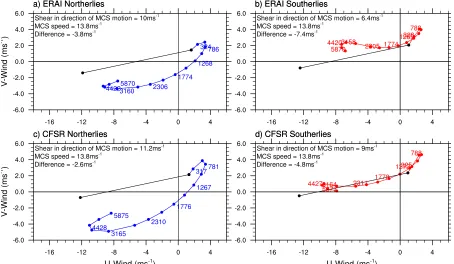
Top-left shows the 2m temperature field at 2007/09/08 11UTC (the time of initiation). top-right shows the terrain and simulated radar reflectivity fields at the same time. The red box shows the region where CI is occurring. The two skew-T log-P diagrams show the environment in the red box 24 hours before initiation (bottom-left) and at the time of initiation (bottom-right). . . 61 Figure 3.10 Hodographs of the 1000–500-hPa wind shear in composite average

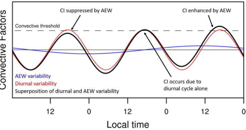
a,b) ERAI and c,d) CFSR waves. Average profiles are in the a,c) norther-lies and b,d) southernorther-lies. Colored numbers show geopotential height of the point. Black lines show the average speed and direction of the QLCS relative to the surface wind. Text shows shear projected in the direction of MCS motion, QCLS speed, and the difference between the two. . . 65 Figure 3.11 Idealized depiction of the super-position of the diurnal cycle with the

AEW variability for enhanced and suppressed CI in different phases of the AEW. . . 68

Figure 4.1 Composite average AEWs in ERAI showing the 650-hPa AEW-scale PV (PVU; shaded) with a,b,c) rotational and d,e,f ) divergent wind vectors (ms−1_{). Base points are a,d) Atlantic, b,e) West Africa, and c,f ) East} Africa. . . 70 Figure 4.2 Meridional gradient in mean JAS PV (shaded) at a,b) 650 hPa, and c-f )

for a 30◦_W-30◦_{E average. Overlaid in contours is the time-mean JAS} a-d) Zonal Wind with dashed contours negative and solid contours positive, and e-f ) Potential Temperature. Contour spacing is 2m s−1 and 5 K respectively. . . 72 Figure 4.3 Composite-average ERAI a,b,c) latitude-longitude cross-sections of

(12)

Figure 4.4 As in figure 4.3 but using CFSR. . . 75 Figure 4.5 Latitude-height cross sections of AEW-scale PV and time-mean

po-tential temperature through the composite average troughs at each base point. Base points a,d) Atlantic, b,e) West Africa, c,f ) East Africa. Plots are shown for a,b,c) ERAI and d,e,f ) CFSR. . . 78 Figure 4.6 Longitude-height cross-sections of AEW-scale PV (shades, PVU) and

AEW-scale diabatic heating (contours, K/day). Representations of diabatic heating are a-f )Q1, g-i)H, and j-l)HL. a-c) are for ERAI and

d-i) are for CFSR. Composite AEWs are at the a,d,g) Atlantic, b,e,h) West Africa, and c,f,i) East Africa base points. Each cross-section is averaged between 5-15N. The green-brown line plots represent TRMM precipitation for the composite ERAI AEWs (top row) and the composite CFSR AEWs (bottom row). . . 79 Figure 4.7 Longitude-height cross-sections through composite AEWs averaged

between 5-15◦_{N showing AEW-scale PV tendency (PVU}_/_{day; shades)} and ¯V · ∇Pw (PVU/day contours). . . 82

Figure 4.8 Longitude-height cross-sections through composite AEWs showing AEW-scale PV (shades, PVU) and selected source terms (contours, PVU/day). All variables are averaged between 5-15◦N. Source terms are a,b,c)∂Pw/∂t +V¯· ∇Pw, d,e,f ) ¯η∂Q1w/∂p, g,h,i)ζw∂Q¯1/∂p. All

contour intervals are 0.005PVU/day. . . 83 Figure 4.9 As in Figure 4.8 but for CFSR. Also the diabatic heating rates areH

instead ofQ1. . . 84 Figure 4.10 Horizontal cross-sections through composite AEWs showing

800-550hPa averaged AEW-scale PV (shades, PVU) and−Vw· ∇P¯. a) and

d) are for the Atlantic base point, b) and e) are for the West base point, and c) and f ) are for the East base point. a,b,c) show ERAI and d,e,f ) show CFSR. . . 86 Figure 4.11 Longitude-pressure cross-sections showing the fractional

contribu-tion of various source terms from equacontribu-tion 2.31 averaged between 4–20◦N for a,c,e,g) ERAI and b,d,f,h) CFSR. Source terms represented are a,b)₋V¯· ∇Pw, c)−η∂¯ Q1w/∂p, d)−η∂¯ Hw/∂p, and e,f )−Vw· ∇P¯.

Grey areas show regions below ground. . . 90 Figure 4.12 Longitude-pressure cross-sections as in Figure 4.11 but for fractional

growth. a,c,e,g) are for ERAI and b,d,f,h) are for CFSR. a,b) show₋Vw· ∇P¯, c) shows₋η∂¯ Q1w/∂p, d)−η∂¯ Hw/∂p, e) shows−ζw· ∇Q¯1, and f ) shows₋ζw· ∇H¯. . . 92

(13)

Figure 5.2 Bar charts showing the fractional contributions to a,b) growth (equa-tion 4.1; per day) and c,d) propaga(equa-tion (equa(equa-tion 4.2; no units) by various PV sources. Sources are averaged over 800-400 hPa and in time. Averages in time are separated into when the wave center was over a,c) land and b,d) ocean. Blue bars are for the 2007-CTRL simu-lation and red bars are for the 2010-CTRL simusimu-lation. . . 101 Figure 5.3 Fractional contribution to growth of perturbation PV (units of per

day) by various perturbation PV sources. Plots are time-pressure cross-sections following the tracked AEW trough center for a,c,e) 2007-CTRL and b,d,f ) 2010-CTRL. Sources shown are fractional con-tribution to growth by a,b)V0_{· ∇}_P_¯_{, c,d)}_V0_{· ∇}_P0_{, and e,f )}_(ζ_{· ∇}_Q

m p)0

(PU, contours). The individual vertical black lines indicate the point at which the trough passes the West African Coast. Note scale is not linear, scale doubles for each color. . . 103 Figure 5.4 As in Figure 5.3 but for fractional contribution to propagation (no

units). . . 104 Figure 5.5 Longitude-pressure cross-sections following the tracked AEW trough

center for a,c,e) 2007-CTRL and b,d,f ) 2010-CTRL. Cross-sections are averaged over an area 250km north and south of the trough center and averaged over the 3 days while the AEWs are solely over land. Variables shown are perturbation PV (PU, contours) and a,b) pertur-bation cloud fraction, c,d) perturpertur-bation microphysical heating, and e,f ) perturbation diabatic PV source using only microphysical heating.106 Figure 5.6 Cross-sections in the 2007-CTRL simulation at times when diabatic

PV production is producing growth (Figure 5.3f ). a,c,e,f ) Horizontal cross sections of maximimum radar reflectivity (shades) and 400-800 hPa averaged perturbation PV (contours). PV contours are at inter-vals of 0.1 PVU. b,d,f,h) longitude-pressure cross-sections of cloud fraction (shades) and perturbation diabatic PV production by micro-physical heating (contours) averaged over longitudes corresponding to the perturbation PV on the left. Diabatic PV source contours are at intervals of 0.25 PVU/day. . . 109 Figure 5.7 As in Figure 5.6 but for the 2010-CTRL simulation. . . 111 Figure 5.8 PV (contours; PVU) and meridional winds (shades; ms−1) averaged

250 km north and south of the tracked AEW vorticity center, and then averaged over the simulation. Figures show different simulations; a) CTRL, b) 2010-CTRL, c) HLFM, d) 2010-HLFM, e) 2007-NOMH, and f ) 2010-NOMH. . . 114 Figure 5.9 Time series of a,b) perturbation PV and c,d) EKE following the tracked

(14)

Figure 5.10 As in Figure 5.9 but for 500-300 hPa. . . 117 Figure 5.11 Average fractional contribution to growth/decay of 800–300-hPa

per-turbation PV following AEW (units of per day). . . 118 Figure 5.12 Three-dimensional conceptual diagram of the moist convective

dy-namics affecting AEWs. Diagram depicts 2 planes, one at the surface and one at the peak level for AEWs. Red and blue shades depict AEW perturbation PV. Orange and green shades indicate condensational heating and evaporative cooling respectively associated with the trail-ing stratiform cloud regions behind MCSs depicted as grey clouds. Generation of positive PV by diabatic processes is depicted by red circles with black outlines. Arrows represent the background zonal wind profile. . . 119

(15)

CHAPTER

1 INTRODUCTION

1.1 Definition

(16)

1.2 Motivations

AEWs are studied for two primary reasons; 1) they are associated with variability in precipi-tation over the West African continent and the Atlantic (e.g. Reed et al. 1977; Laing et al. 1999; Mathon et al. 2002; Fink and Reiner 2003) and 2) they are the source of a majority of tropical cyclones (TCs) in the Atlantic (e.g. Avila and Pasch 1992). The benefits for West African countries primarily lie in the former while the significance for other countries (such as those in the Caribbean and North America) typically lie in the latter.

Many studies have shown a clear association between AEWs and precipitation or strong mesoscale convective systems (MCSs) over West Africa. Mekonnen et al. (2006) showed that the 2-6 day time scale accounted for 25-35% of the variance of convection over West Africa. Meanwhile Fink and Reiner (2003) showed that around 40% of MCSs in the WAM system are forced by AEWs. Further, Laing et al. (2012) showed that long-lived intense convective events over West Africa occur with a 2-3 day periodicity and then Laing et al. (2011) showed that the modulation of convection by larger scale disturbances is a primary source of variability. These strong convective events and large variations in precipitation affect West African communities through public safety, agriculture, and energy production, just to name a few. Thus the dynamics of AEWs are clearly of importance for West African communities.

A survey of the National Hurricane Center (NHC) TC reports (published in Russell et al. 2017) showed that over 70% of Atlantic TCs have origins related to AEWs. This fraction can be separated into a contribution where AEWs were the incipient disturbance for TCs (genesis fraction; GF) and a contribution where AEWs played a positive role in organizing moist convection but were not the main disturbance (contribution fraction; CF). Figure 1.1a shows the GF (red) and CF (blue) for all surveyed years. The average GF is 0.61 and the average contribution fraction is 0.11. This indicates that 61% of TCs form directly from AEWs, while AEWs contribute positively to the formation of a further 11% of TCs. This equates to approximately 13 TCs per season where AEWs played a positive role in their formation (Figure 1.1c). These fractions and the corresponding numbers (genesis number and contribution number; GN and CN respecitvely) are also slightly higher for hurricanes (figures 1.1b and 1.1d) and even higher for major hurricanes (Landsea 1993). In addition, non-developing easterly waves propagate into the north Pacific Ocean where they often become precursors for TCs (Molinari et al. 2000).

(17)

(18)

2017, three major hurricanes (Harvey, Irma, and Maria) caused significant loss of life, as well as multi-billions of dollars in damage, across the Caribbean islands and the United States.

The first of these hurricanes, Harvey, formed from an AEW in the tropical Atlantic, tracked westward across the lesser Antilles as a tropical storm and dissipated in the southern Caribbean sea, before reforming in the Gulf of Mexico, and rapidly intensifying into a major hurricane. Harvey made landfall in southern Texas as a Category 4 Hurricane and resulted in up to 60 inches of rainfall falling around the Houston area causing unprecedented flooding. Harvey resulted in 69 fatalities and an estimated $125 billion dollars in damage (Blake and Zelinsky 2018).

Irma formed near the Cape Verde Islands from an AEW and rapidly intensified into a Category 5 hurricane, maintaining major hurricane strength for the longest of any major hurricane in the Atlantic basin. Irma caused 139 deaths across the Caribbean Islands and caused multi-billions of dollars in damage across the region, destroying up to 95% of structures on some islands (Cangialosi, Latto, and Berg 2018).

Maria formed from an AEW in the tropical Atlantic, rapidly intensified into a Category 5 hurricane, and made two landfalls in Dominica and Puerto Rico, both as a Category 5 hurricane. The official death toll in Puerto Rico is now reported to be well into the thousands including many indirect deaths as a result of the severe damage to the islands infrastructure. The total cost on all islands effected is estimated to be around $100 billion (Pasch, Penny, and Berg 2018). Combined, these three hurricanes demonstrate the severe effects on life, infrastructure, and economies that originate from AEWs.

(19)

(20)

1.3 Dry Dynamics of AEWs

The focus of early research on the growth and maintenance of AEWs was primarily on the dynamical instability of the AEJ (Carlson 1969; Burpee 1974; Reed et al. 1977; Norquist et al. 1977). These studies suggested that AEWs grow through the baroclinic and barotropic extraction of energy from the AEJ. This conclusion was based on the fact that the background state over West Africa met the conditions for such instabilities presented by Charney and Stern (1962); a reversal in the meridional gradient of background potential vorticity (PV). These and later studies (e.g. Thorncroft and Hoskins 1994) essentially described AEWs as growing Rossby waves (RWs), with the AEJ as the source of energy and the waveguide.

In dry idealized simulations with a basic state characterized by a simple easterly jet, Thorncroft and Hoskins (1994) produced waves that resembled the synoptic features ob-served in AEWs. The major difference was in the vertical velocity that was too weak and produced an unrealistic pattern. In this system, they showed that the dynamics are dom-inated by the interaction between waves on the positive and negative potential vorticity (PV) gradients associated with the background flow. The conclusion of Thorncroft and Hoskins (1994) was consistent with Burpee (1972), who first recognized the potential for mixed barotropic-baroclinic instability of the AEJ from observations.

Since then, a number of studies have shown that dry barotropic and baroclinic insta-bilities of the AEJ are insufficient to explain the growth and maintenance of AEWs (e.g. Hsieh and Cook 2005; Hall et al. 2006). In particular Hall et al. (2006) showed that given a modest amount of damping with an idealized AEJ, the normal modes of the AEJ were effectively neutralized. This suggests that some other process must exist that allows for the maintenance and growth of AEWs as observed.

1.4 Influence of AEWs on Convection

A strong relationship between AEWs and convection was detailed by Payne and McGarry (1977). Later, Duvel (1990) used Meteosat data and ECMWF analyses to show that the strongest deep convection occurs at, and ahead of, the wave trough over land, before transitioning into the trough over the East Atlantic. He also noted that convection coincided with synoptic scale divergence in the upper-levels and variations in the thermodynamic profile on scales similar to the AEW. This work hinted at the possibility that AEWs produce forcing for ascent resulting in moist convection.

(21)

convection and AEWs. These studies highlight the possibility for convection to have strong interactions with AEWs. Many other studies have also associated convection with AEWs (e.g. Diedhiou et al. 1999; Gu et al. 2004). These studies noted that convection primarily occurs in the northerlies and trough over land, and the trough over ocean, as in Duvel (1990). Combined, these studies present clear evidence that AEWs have an organizing effect on convection.

However, this organizing effect very rarely produces moist convection that is linearly coupled to the AEW. Diedhiou et al. (1999) and Gu et al. (2004), showed that convection often moves through the wave as it crosses west Africa. Further Laing et al. (2008) showed that the distribution of propagation speeds of observed cold cloud episodes (e.g. MCSs) does not well match the phase speeds of AEWs tracked in the National Center for Environmental Prediction (NCEP) Global Final Analysis. Further, Cifelli et al. (2010) used data from the AMMA and NAMMA field campaigns to examine one particular AEW during 2006. They found that convection was not significantly impacted with the passage of this AEW. These studies highlight the fact that the relationship between AEWs and MCSs is complex.

Thorncroft and Hoskins (1994) showed that in an idealized adiabatic wave, there are clear ascent and descent regions. Later, Kiladis et al. (2006) used modified Q-vectors in composite ERA-40 reanalysis waves to show that AEWs produce adiabatic forcing for ascent ahead of the trough. While the Quasi-geostrophic (QG) forcing for ascent broadly coincided with fields of vertical motion and outgoing long wave radiation (OLR), there was a slight phase lag between the forcing for ascent and the response. Furthermore, they found that the QG forcing was not uniformly successful in accounting for the vertical motion and precipitation in the wave.

(22)

(23)

1.5 Influence of Convection on AEWs

Norquist et al. (1977) suggested that latent heating produced by convection can be a dom-inant factor for the growth and maintenance of AEWs over West Africa. Using a vorticity budget for a composite AEW from the GATE experiment, Shapiro (1978) found that with-out a simple parameterization for cumulus the vorticity source in AEWs may be under-represented. Thorncroft and Hoskins (1994) investigated the role of diabatic effects in a linear model of AEWs. With a simple parameterization of latent heat release, the most unstable modes became less dominated by barotropic energy conversions and the growth rates were increased. Further, the vertical velocities were found to better match observed patterns and magnitudes. They concluded that the role of latent heating is important in increasing the baroclinic energy conversions, and also in determining the synoptic struc-ture. These studies were the first to show that convection was important for the growth and maintenance of AEWs.

However, the exact mechanism through which convection enhances AEWs is still a debated topic. An analysis of one simulated AEW by Berry and Thorncroft (2005) indicated that convection has notable effects on the AEW at multiple stages during its growth and maintenance. They argued that PV generated by convection coupled with the AEW supports the growth of the AEW via baroclinic processes. Then, convection near the west African coast maintains the AEW after dry baroclinic processes have weakened. More recently, Berry and Thorncroft (2012) produced an ensemble of simulations to demonstrate that convection is important for the maintenance of AEWs. An energy budget that computed diabatic (convective) and adiabatic (instability) forcing, concluded that the two were of the same order of magnitude. Comparison of the results with a dry simulation (convective parameterization switched off ) showed that the AEW weakened substantially. These results are consistent with those of Schwendike and Jones (2010), Janiga and Thorncroft (2014), and Poan et al. (2014) who showed that convection acts to enhance vorticity, PV, and momentum respectively in the low-to-mid levels over West Africa. All in all, these studies support the idea that convection enhances low-to-mid level rotation through moist baroclinic processes.

1.6 Convection and Synoptic Systems

(24)

involved in DRWs and CCEWs, with a view to applying these to AEWs later.

A DRW is a wave for which the diabatic (convective) generation of low-level PV, governs the evolution in a manner similar to advection of PV in Rossby waves (e.g. Raymond and Jiang 1990). A majority of research (Parker and Thorpe 1995; Moore and Montgomery 2005) on DRWs has focused on the mid-latitudes and the genesis and maintenance of Diabatic Rossby Vortices (DRVs) (a closed circulation counterpart to the DRW). As defined by Shih (2012), a DRV is a diabatically dominated, moist baroclinic disturbance, in the absence of discernible upper tropospheric forcing. A depiction of the DRV in mid-latitude mean westerlies is shown in Figure 1.4. The specific propagation mechanism can be described as follows. A positive PV anomaly generates a balanced circulation with southerlies to its east. In a moist-baroclinic zone with isentropes sloping upward to the north, these southerlies generate dry adiabatic ascent which then triggers moist convection. The associated latent heating generates a low-level positive PV anomaly to the east of the previous PV anomaly. This propagates the system eastward.

Figure 1.4: A schematic of a DRV in mean westerlies adapted from Parker and Thorpe (1995). a) depicts a current time and b) depicts a later time. Current positive PV (solid red circles), past positive PV (dashed pink circle), southerlies (X), ascent (w), and diabatic heating (Q) are shown in association with the cloud distribution.

(25)

layers. Interactions between the PV anomalies on various upper and lower layers produce baroclinic instability when they exhibit a favorable upshear tilt. It is of interest to adapt this framework to the case of the mid-level AEJ and the attendant dry and moist components associated with the AEW.

A number of studies have speculated that the process through which AEWs interact with convection is representative of a DRW (e.g. Moore and Montgomery 2005; Berry and Thorncroft 2005, 2012; Tomassini et al. 2017). These studies have, however, not provided any analysis to support their claim. It is possible that the DRW model is applicable to AEWs since part of their life cycle is spent in a region of relatively large (for the tropics) meridional temperature gradient, they induce adiabatic ascent ahead of the trough, and that a balanced response to moist convection is possible at the latitude of the AEWs.

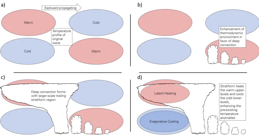
Another model for coupling of synoptic scale waves to convection is stratiform instability (Mapes 2000). This is typically used for convectively coupled equatorial waves but some aspects may be of some relevance for AEWs. The schematic in Figure 1.6 illustrates a highly simplified version of the process for an eastward propagating wave, illustrating some of the properties that may be pertinent to AEWs. As the wave propagates eastward it’s thermodynamic structure enhances CAPE, priming the thermodynamic environment in favor of convection. As congestus builds, developing convection slowly removes the convective inhibition (CIN) (Figure 1.6b). Deep convection then forms once CIN has been removed and the first phase of the wave has passed. This leaves a region of trailing stratiform cloud in the next phase of the wave (Figure 1.6c). Finally, the second-baroclinic structure of heating, as a result of the stratiform cloud, heats the upper-levels and cools the lower-levels. This further enhances the thermodynamic structure of the wave (Figure 1.6d).

Kuang (2008) presented a modified version of the stratiform instability mechanism that couples moist convection to the wave through moisture convergence, rather than through the removal of CIN. This is referred to as the moisture-stratiform instability. The mechanism for enhancement of the wave by convection (i.e. heating and cooling from stratiform cloud) remains the same here.

1.7 Open Questions and Theories

(26)

(27)

Figure 1.6: Vertical cross-sections (x-z) illustrating key properties of the stratiform insta-bility process.

to answer these questions. Each section will conclude by summarizing the questions I aim to answer.

1.7.1 Influence of AEWs on Convection

As noted earlier in this chapter, and highlighted by the studies of Diedhiou et al. (1999), Gu et al. (2004), Laing et al. (2008), and Cifelli et al. (2010) moist convection is rarely linearly coupled to the AEW. Thus a first step toward understanding their interrelationship is better characterizing the moist convection present within the AEW envelope. We therefore need to establish the overall structure, motion, and dynamics of moist convection. This will include understanding how it is initiated and maintained. Once moist convection has been characterized, it is then possible to relate it to the AEW and interpret how factors influenced by the AEW, may enhance moist convection.

(28)

un-derstanding of how AEWs force moist convection needs to examine whether the initiation of moist convection such as MCSs, can be directly attributed to dry adiabatic ascent.

Exactly why there is a variation in CAPE and moisture associated with the AEW is unclear. Two possibilities arise. The first is that the AEW directly enhances CAPE and moisture. These could occur through advection of warm and moist surface air. In such a case, the temperature and moisture distribution of the background environment plays an important role. The second is that this variation in CAPE and/or moisture is a biproduct of the coupled convection. For example, CAPE is reduced as it is consumed by convection. Thus, in the wake of long-lived MCSs (i.e. those that last longer than a diurnal cycle) it may take a couple of days for CAPE to recover. Long-lived MCSs are often observed coincident with the AEW (Laing et al. 2008). To gain a complete picture of how the thermodynamic and moisture environments of the AEW affect moist convection we need to understand whether these are a product of the AEW or the convection.

In summary we will attempt to address the following questions with regard to the role AEWs play in modifying convection:

1. What are the characteristics of moist convection within the AEW envelope and how do they relate to the AEW?

2. Are the thermodynamics and moisture a result of the AEW or a biproduct of the convection?

3. Which factors influenced by the AEW (e.g. moisture convergence, thermodynamic priming and kinematic priming of the environment, and adiabatic forcing for ascent) are important in initiating and maintaining moist convection?

1.7.2 Influence of Convection on AEWs

(29)

When considering PV sources, deep convection typically enhances PV in the low-levels where the vertical latent heating gradient is strongest. Thus a question that remains is how convection enhances PV in the mid-levels. Janiga and Thorncroft (2016) showed that there are elevated stratiform cloud fractions in the trough of AEWs over West Africa and Janiga and Thorncroft (2013) showed that there is mid-level generation of PV. A number of studies have shown that MCSs are often associated with mesoscale convective vortices (MCVs) in the mid-levels (Velasco and Fritsch 1987; Menard and Fritsch 1989; Laing and Fritsch 1993; Skamarock et al. 1994). Fritsch et al. (1994) and Davis and Weisman (1994) showed that MCVs occur due to the mid-level generation of PV by stratiform cloud regions associated with MCSs. Our expectation is therefore that it is the statiform cloud, not the deep convection, that leads to enhancement of the AEW PV anomaly. However, a direct link between stratiform cloud, the PV generation associated with MCVs, and the maintenance and propagation of AEWs is yet to be shown.

Further, Berry and Thorncroft (2012) found that adiabatic and diabatic sources of energy in AEWs were comparable. This quantitative difference can arguably be better understood using PV. To understand the importance of moist convective processes, PV tendencies as a result of latent heating need to be put into context relative to other diabatic (i.e. radiative and surface processes), adiabatic, and frictional sources. Here, we expect that the sources of PV from advection and latent heating will be comparable in magnitude.

Finally, very few studies have examined AEWs in simulations where moist convection is limited to various degrees. Such an experiment may help explain how convection modifies AEWs. If an AEW can be maintained in some form after the convection has ceased then the wave is not completely reliant on diabatic processes. Thorncroft and Hoskins (1994) examined waves on an idealized AEJ with and without a simple convective parameterization. The biggest difference they found was that the vertical velocity pattern varied between the two. Meanwhile, Berry and Thorncroft (2012) used full physics simulations with the Weather Research and Forecasting model (WRF) to examine an AEW with and without parameterized convection. They found that the AEWs mid-level signature weakened considerably after the convective parameterization was switched off. However, they only focused on the mid-level AEW signature and neglected to examine the entire wave structure. These studies present contrasting views and such studies need to be analyzed in detail. We hypothesize that the AEW can be maintained by adiabatic processes but will have weaker low-to-mid level perturbations.

(30)

1. What is the structure of diabatic PV tendencies relative to the AEW? And how do they compare to adiabatic PV tendencies in an AEW?

2. How does the structure of convection lead to mid-level rotation on the scale of the AEW?

3. Does an AEW exist without convection present? And if so, what is the difference in AEW structure and why?

1.7.3 A Complete Model for AEW-Convection Interaction

Describing the AEW-convection interaction with a detailed conceptual model is the ultimate goal of this study. To present this model, the answers to the previous questions will need to be combined with current understanding and examples of other convectively coupled waves.

As previously discussed, the DRW mechanism has been suggested as one such mecha-nism for the AEW-convection interaction. While AEWs exist in a similar moist baroclinic environment, the DRW mechanism must be adapted for a mid-level wave in easterly shear. There are a number of issues here. The first two are the mechanism coupling convection to AEWs and the mechanism generating PV in the mid-levels. Both issues have been discussed in the previous sections.

Another major issue with the applicability of the DRW mechanism to AEWs is the scale separation between convection and AEWs. How are PV anomalies on the scale of the AEW generated by deep convection? In the mid-latitudes, DRWs are typically smaller in scale than their dry counterparts, primarily because they are driven by smaller scale convective processes. However, AEWs are much larger than individual convective systems over West Africa. Typically over West Africa there is more than one convective system present at any given time. It’s therefore possible that the combination of all the convective systems ahead of the trough at any given time generates a PV anomaly on the scale of the AEW. This, however, is yet to be shown.

(31)

convection transitions from sheared MCSs over Africa to hot towers in the trough over the Atlantic.

Stratiform instability is a mechanism for the coupling of convection to, and subsequent enhancement of convectively coupled equatorial waves. AEWs are typically likened more to QG Rossby waves evolving in a baroclinic atmosphere. Thus stratiform instability is not a mechanism through which we could completely explain the AEW-convection interaction. However, as can be seen on examination of the average thermodynamic and convective structure of an AEW (e.g. Kiladis et al. 2006, Figure 11) over West Africa, the AEW exhibits a very similar thermodynamic and convective structure to that presented in Figure 1.6. This raises the possibility that some aspects of the stratiform instability may be applied to AEWs.

The mechanism coupling convection to the wave in stratiform instability is the wave’s variability of CIN and CAPE. In the DRW the coupling mechanism is adiabatic forcing for as-cent. If, on the other hand, AEWs organize convection via horizontal moisture convergence, as presented by Tomassini et al. (2017), the coupling mechanism for moisture-stratiform instability (Kuang 2008) may be relevant for AEWs. This study will introduce and discuss whether some aspects of stratiform instability may be applied to the AEW-convection interaction.

In summary we will attempt to combine the knowledge gained in this study into a complete conceptual model of AEW-convection interaction by addressing the following questions:

1. What aspects of the DRW mechanism and/or stratiform instability are present in AEWs?

(32)

CHAPTER

2 METHODS

2.1 Data

2.1.1 Representation of AEWs

When examining the AEW-convection relationship we have three broad categories of datasets available. These are observations (either in-situ or remote), simulations or reanaly-ses with parameterized convection, or high-resolution simulations with explicit convection. Typically, in-situ observations over Africa are not able to provide high enough temporal and spatial resolution to study a relationship with convection. For certain variables such as precipitation, satellite-borne measurements such as the National Aeronautics and Space Administration (NASA) Tropical Rainfall Measurement Mission (TRMM; Huffman et al. 2007) or the Global Precipitation Mission (GPM) do some work toward filling in the gaps. On short temporal scales field programs such as AMMA also provide more data. However, none of these platforms provide a detailed enough picture, either in space, time, or in variables (i.e. thermodynamic, moisture, and kinematic variables) to assess the complete AEW-convection interaction.

(33)

consis-tent datasets, that can be analyzed in detail. However, they do not always replicate reality appropriately. Janiga and Thorncroft (2016) aptly summarized the issues with recent exam-inations of AEWs that primarily employ simulations or reanalyses with parameterized or superparameterized convection. Such models typically underestimate the rain rate in the northerlies and overestimate the rain rate in the trough and southerlies (e.g. Skinner and Diffenbaugh 2013; McCrary et al. 2014; Crétat et al. 2015). These representations also fail to resolve MCSs which account for a majority of the convection over West Africa (Janiga and Thorncroft 2014). An accurate representation of MCSs is important to diagnose differences in vertical profiles of heating and the level of PV generation.

Simulations with explicit convection (i.e. convection-permitting at 4km or lower grid-spacing) are able to represent MCSs. Pearson et al. (2014) also showed that convection-permitting simulations are much better at simulating the diurnal cycle over West Africa. Since MCSs are strongly modulated by the diurnal cycle (Laing and Fritsch 1993), convection-permitting simulations are important for both the initiation and intensity of MCSs. The only study that uses convection-permitting simulations to examine convection in relation to AEWs is Schwendike and Jones (2010). In this study they examined just two MCSs, only resolving convection for a limited period of the lifetime of an AEW and this study is therefore limited in scope.

Our approach in this study will be to use all three types of datasets in conjunction with each other where and when possible. We expect that explicit representation of MCSs may be required to correctly represent the phase relationship between AEWs and convection and the correct structure of heating profiles in MCSs. Thus we will make heavy use of high resolution simulations.

2.1.2 Reanalyses and Precipitation

(34)

parameters such as heating rates can be highly sensitive to the various parameterizations. The grid-spacing of the datasets are approximately 0.8◦for ERAI and 0.5◦for CFSR. Both will sufficiently resolve synoptic-scale features such as the AEW but will not resolve mesoscale features such as Mesoscale Convective Systems (MCSs).

Precipitation is represented by the TRMM Multi-Satellite Precipitation Analysis (TMPA-RT) dataset. All results in this study are based on these datasets from the period 1998-2010. This period is chosen since this is the only period for which all the above datasets (ERAI, CFSR, and TRMM) overlap temporally.

2.1.3 Convection Permitting Simulations

Control Simulations

Simulations are performed using the Weather Research and Forecasting model (WRF-ARW version 3.9.1.1; Skamarock et al. 2005). The domain setup is shown in Figure 2.1. A 36 km spacing outer domain is used with inner domains of 12 km and 4 km spacing. This setup is used to down-scale the initial conditions, the ERAI, with a grid-spacing of approximately 80 km, to a convection-allowing resolution. Two different AEWs are simulated, one from 2010 between the 19th-28th August (that lead to the genesis of Hurricane Earl) and one from 2007 between 6th-17th September (that did not lead to the genesis of a TC).

(35)

(36)

advanced interactions with clouds (Price et al. 2014). The simulations are initialized with a Dolph digital filter run backward and forward two hours to remove initial imbalances in the model initial conditions. It is found that this combination of filtering and parameterization schemes produces the best representation of the AEWs, as represented by ERAI and TRMM data. Filtering also allows for the initial conditions, especially those that are adjusted in sensitivity studies that will be described, to be balanced prior to the simulation start.

Table 2.1: Parameterization schemes used in the 2007 and 2010 simulations.

Parameterization Scheme WRF Option Cumulus Modified Tiedtke 6

Microphysics Thompson 8

Boundary Layer Shin-Hong 11

Surface Layer Revised MM5 1

Land Surface Noah LSM 2

Radiation (SW & LW) RRTMG 4

A control simulation is run for each AEW (hereafter referred to as CTRL). Time-longitude diagrams of 650hPa meridional winds and precipitation from the CTRL simulations are shown in Figures 2.2c and 2.2d for the 2007 and 2010 AEWs respectively. To provide a valid comparison we regrid the simulations to the ERAI and TRMM grids for winds and precipitation respectively. CTRL simulations are favorably comparable to the "observed" AEWs. All the AEWs follow similar tracks as can be seen by comparing the CTRL tracks to the ERAI meridional winds. Further, meridional winds intensify and decay at similar times between the CTRL simulations and ERAI observations. Finally TRMM and CTRL precipitation is similar with consistent precipitation in the northerlies of each AEW and weaker, if any, precipitation in the southerlies of each AEW. The only qualitative differences are slightly faster AEWs in the ERAI compared to the CTRL, especially over the ocean. While it is helpful to have a simulation that very closely matches reality, the goal of the study is not to recreate the AEW exactly, but to simulate an AEW that is appropriately realistic and examine it’s relationship with convection. Given this, we believe these simulations suitably recreate the AEWs.

(37)

(38)

WRF. This simulation utilizes an outer domain with 12km grid spacing similar to the 36km domain in Figure 2.1, and an inner domain with 4km grid spacing similar to the 4km domain in Figure 2.1. Initial and boundary conditions were provided by the 1/4◦_{Global Forecast} System (GFS) at forecast hour 0. The only other difference from other simulations is the use of WDM6 microphysics instead of Thompson. This simulation also favorably replicates the AEW in question, relative to ERAI and GFS analyses (not shown). Unfortunately, for data storage reasons, this simulation could not be retained and the information gleaned from it is only used in a limited manner in Chapter 3 with the purpose of supporting data from the other simulations.

Sensitivity Studies

A series of sensitivity studies are performed to examine the difference between AEWs with and without the effects of convection. Two different sensitivity studies are carried out. The first removes the condensational heating produced by the microphysics scheme. Such simulations are denoted NOMH hereafter. Since there is no active convection scheme in the 4 km domain this represents a removal of any and all condensational heating. These simulations produce close to zero precipitation. This lack of precipitation can be explained through parcel theory. Assuming a rising parcel, once a parcel reaches the lifting conden-sation level (LCL) in normal atmospheric conditions it would begin rising at the moist adiabatic lapse rate (MALR) due to the release of heat by condensation. However, since there is no condensational heating in these simulations, rising parcels continue to rise at the dry adiabatic lapse rate (DALR). Since the DALR is much steeper than that of the MALR, rising parcels would be much cooler than the environment in most cases. Thus rising parcels in these simulations are typically stable to convective motions. Since most precipitation over West Africa in the summer originates from deep convection, precipitation is therefore vastly reduced in the simulations.

(39)

Table 2.2: Summary of all simulations. M represents all mixing ratio variables and MP stands for microphysics. Times are in UTC.

Abbreviation Date and Time Modification CTRL-2007 6/9 00Z – 17/9 00Z None

HLFM-2007 8/9 12Z – 17/9 00Z M reduced 50% at first time

NOMH-2007 8/9 12Z – 17/9 00Z Zero temperature tendency in MP scheme CTRL-2010 19/8 00Z – 28/8 00Z None

HLFM-2010 20/8 12Z – 28/8 00Z M reduced 50% at first time

NOMH-2010 20/8 12Z – 28/8 00Z Zero temperature tendency in MP scheme CTRL-2017 3/8 00Z – 13/8 00Z None

relative humidity and surface moisture, the dew point is lower, and LCLs are higher. As a result, it is harder for convection to realize convective available potential energy (CAPE) through moist convection, although not impossible. This leads to much less precipitation. This is especially prevalent later in the simulations when some moisture has been reintro-duced by evaporation and transpiration from the land surface scheme. Multiple factors were tested (0.9, 0.7, 0.5, 0.25, 0) but an examination of these showed that 0.5 presented the best way to limit convection while at the same time maintaining an environment that reflected reality.

(40)

Analysis of Simulations

In order to discern characteristics of the AEWs from these high resolution simulations, we utilize a number of techniques in order to better represent AEWs. To obtain data repre-sentative of the AEW, variables are first smoothed in space using a 500 km wide Gaussian weighted window. This provides us with variables that are smoothed to an effective reso-lution of 3000-4000 km (the AEW scale). In this case variables on the scale of convection should have been smoothed out. From this we then calculate time-mean averages defined as the mean of all output times over the whole simulation at any given location. We then define perturbations as the difference between any filtered variable and its time mean fil-tered variable at any given location. This allows for the removal of the background features (such as the AEJ) from perturbation variables. Since AEWs are the dominant synoptic scale pattern in the region, this gives us our best estimate of the variables that represent the AEW.

2.2 Potential Vorticity

PV is a useful quantity with which to analyze AEWs as it combines both thermodynamic and kinematic properties of the wave into one variable. More specifically a PV tendency equation or budget as we shall describe it herein, directly links diabatic heating (or more accurately the gradients of diabatic heating) to generation of PV (Hoskins et al. 1985). Through PV we can therefore directly quantify the contribution of convection to the AEW. Further, given an appropriate balance condition (such as quasi-geostrophic or nonlinear balance), PV can be inverted to obtain the balanced wind and mass fields. Thus PV also describes the balanced part of the circulation, and by understanding it’s sources and sinks, it is possible to describe the balanced dynamics of AEWs.

Many approaches to understand the role of convection in modifying AEWs have used energy budgets to understand AEW growth (e.g. Hsieh and Cook 2007; Berry and Thorncroft 2012; Poan et al. 2014). However, energy budgets do not cleanly separate the adiabatic and diabatic processes. Moist convective and dry baroclinic energy sources are typically pooled into the baroclinic term, making it difficult to understand whether the growth is through dry or moist baroclinic processes. Thus an analysis of PV in the AEW represents a useful addition to the current understanding strongly focused on energetics.

(41)

reinforces the AEW through diabatic PV generation between 500-800 hPa. Given that there are distinct diabatic sources of PV in the low-mid levels of AEWs it is important to put these in context with their adiabatic counterparts, as was discussed in the introduction.

2.2.1 Isobaric analysis

Here we derive a potential vorticity (PV) budget in the presence of non-conservative effects of diabatic heating. For such an analysis, isentropic coordinates are typically used since PV takes a relatively simpler form and diabatic heating is directly related to the cross-isentropic pseudo-vertical motion. However, here we use isobaric coordinates for the analysis for a variety of reasons. First, isentropes in the vicinity of the AEW track have steep slopes relative to geometric or isobaric surfaces. This is a result of the intense heating of the surface layer over the Sahara Desert and relatively cooler air over the Gulf of Guinea. Steeply sloping isentropes lead to two main problems. First comparing AEW PV to well understood and well documented features in the vicinity of AEWs is difficult as these features are typically defined on isobaric surfaces. Second, when isentropes intersect the surface there are now sources of PV on isentropes. Furthermore, since we desire to examine the full 3-D structure of the wave, including near the surface, the choice of a vertical co-ordinate does not make a major difference in practice.

2.2.2 Fundamental Equations

The primitive equations on isobaric coordinates (Vallis 2006, pg. 79, eqn. 2.153) are:

DV~ D t =−f

ˆ

k×V~−∇~Φ+F~, (2.1)

Dθ D t =

Jθ cpT

=Q, (2.2)

~

∇ ·U~=∇ ·~ V~+∂ ω

∂p =0, (2.3)

∂Φ

∂p =−α (2.4)

(42)

2.4 is hydrostatic balance.

2.2.3 Derivation of an Isobaric Vorticity budget

If we separate equation 2.1 into its zonal and meridional components we obtain:

∂u

∂t +u

∂u

∂x +v

∂u

∂ y +ω

∂u

∂p =f v−

∂Φ

∂x +Fx, (2.5)

and:

∂v

∂t +u

∂v

∂x +v

∂v

∂y +ω

∂v

∂p =−f u−

∂Φ

∂ y +Fy, (2.6)

We can define a hydrostatic absolute vorticity in isobaric coordinates as:

~

η=f −iˆ∂v

∂p +jˆ

∂u

∂p +

ˆ

k

∂_v ∂x −

∂u

∂y

(2.7)

We can form a three dimensional vorticity equation by taking₋_∂∂_p(2.6)for the ˆi component,

∂

∂p(2.5)for the ˆj component, and∂∂x(2.6)−∂∂y(2.5)for the ˆk component. Further, also using

equation 2.3 we obtain:

Dη~ D t =

∂ ~η

∂t + (U~·∇~)η~= (η~·∇~)U~+∇ ×~ ∇p~ Φ+∇ ×~ F~ (2.8)

whereη~is the absolute vorticity vector. This equation is our vorticity budget in isobaric coordinates.

2.2.4 Derivation of an Isobaric Potential Vorticity Budget

Now we wish to combine the vorticity equation we have obtained with the thermodynamic information we have, in order to obtain a PV equation. Operating∇~θ·on equation 2.8 gives:

~

∇θ · D

D tη~=∇~θ·(η~·∇~)U~+∇~θ·(∇ ×~ ∇p~ Φ) +∇~θ·∇ ×~ F~

= (η~·∇~)U~·(∇~θ) +∇~θ·∇ ×~ F~

(2.9)

It’s not immediately clear here why the solenoidal term vanishes. We can write:

~

∇pΦ=∇~Φ−kˆ∂ φ

(43)

and then the solenoidal term becomes:

~

∇θ·(∇ ×~ ∇p~ Φ) =∇~θ ·∇ ×~ ∇~Φ−∇~θ·∇ ×~ kˆα=−∇~θ ·∇ ×~ kˆα

=∇~θ ·kˆ×∇~α=∂ θ

∂y

∂ α ∂x −

∂ θ ∂x

∂ α ∂y

(2.11)

since∇ × ∇=0.θ andαcan both be expressed as functions of temperature,T(x,y,p)and pressure, p. But we are holding pressure fixed in the partial differentials. This means that bothθ andαare only a function of temperature on an isobaric surface. Thus the solenoidal term should be identically zero. This can be confirmed by using the expressions forθ and αas:

θ =T p0 p

R cp

(2.12)

and

α=RT

p (2.13)

and then the solenoidal term becomes:

R p

p0

p

R cp∂T

∂y

∂T

∂x −

∂T

∂y

∂T

∂x

=0 (2.14)

Now operatingη~_·_∇~ on the thermodynamic (equation 2.2) gives:

~ η·∇~Dθ

D t =η~·∇~Q (2.15)

Using the product rule, we can write the left hand side of equation 2.15 as:

~ η·∇~Dθ

D t =η~·∇~

∂ θ

∂t +U~·∇~θ

=η~· ∂

∂t∇~θ+η~·∇~(U~·∇~θ)

=η~· ∂

∂t∇~θ+η~·(U~·∇~)(∇~θ) + (η~·∇~)U~·(∇~θ)

=η~· D

D t∇~θ+ (η~·∇~)U~·(∇~θ)

(44)

Substituting equation 2.16 in to equation 2.15 gives:

~ η· D

D t∇~θ =−(η~·∇~)U~·(∇~θ) +η~·∇~Q (2.17)

Adding equations 2.17 and 2.9 gives a combined vorticity and thermodynamic equation:

~ η· D

D t∇~θ +∇~θ· D D tη~=

D

D t(η~·∇~θ)

=−(η~·∇~)U~·(∇~θ) + (η~·∇~)U~·(∇~θ) +η~·∇~Q

+∇~θ·(∇ ×~ ∇p~ Φ) +∇~θ ·∇ ×~ F~

=η~·∇~Q+∇~θ ·∇ ×~ F~

(2.18)

Multiplying through by gravity:

D

D t(−gη~·∇~θ) =−gη~·∇~Q−g∇~θ·∇ ×~ F~. (2.19)

and defining P, the isobaric PV as:

P =−g(η~·∇~θ), (2.20)

Equation 2.18 then becomes the PV budget:

D P

D t =−gη~·∇~Q−g∇~θ ·∇ ×~ F~ (2.21)

This equation states that isobaric PV is conserved under adiabatic, frictionless, and hy-drostatic flow. We can expand equation 2.21 by stating that the relative vorticity vector is

~ζ=S~+ζwhere S is the horizontal components of vorticity (the shear) andζrepresents the vertical component (in isobaric coordinates):

∂P

∂t

|{z} A

=−V~·∇~P

| {z } B

−ω∂P

∂p

| {z } C

−g

~

S·∇~Q

| {z } D

+(ζ+f)∂Q

∂p

| {z } E

−g∇~θ ·∇ ×~ F~

| {z } F

. (2.22)

(45)

2.3 Diabatic Heating Rates

A key variable required for our analyses is the diabatic heating rate, Q. Since ERAI does not provide diabatic heating rates, this is estimated using the thermodynamic residual (Yanai et al. 1973; Hagos et al. 2010):

Q1=

Dθ D t =

∂ θ ∂t +u

∂ θ ∂x +v

∂ θ ∂ y +ω

∂ θ

∂p. (2.23)

CFSR and WRF do provide heating rates as output from the various parameterization schemes. The sum of all diabatic heating from the parameterization schemes is denotedH. We will also examine the role of diabatic heating sources from the sum of all convective (shallow and deep) and microphysical processes (denotedHL), the sum of both longwave

and shortwave radiative schemes (denotedHR), and the boundary layer scheme (denoted

HB). In the case of our WRF simulationsHL is simply the microphysical heating rate since

there is no cumulus scheme active in our 4km domain of interest. CFSR provides these heating rates on a 1◦_{grid. A bilinear interpolation is used to interpolate these to the same} 0.5◦_{grid as the rest of the CFSR variables.}

2.4 Perturbation PV Budget

Returning to the PV budget (equation 2.22), the source terms can be further separated by splitting variables into their time-mean and perturbation components (e.g.V =V¯+V0_). This yields a perturbation PV equation where source terms are separated into products of time-mean and perturbation variables:

∂P0

∂t =−V¯· ∇P

0

−V0· ∇P¯−V0· ∇P0−

ω∂P

∂p

0

−

gη~·∇~Q

0

−

g∇~θ ·∇ ×~ F~

0 .

(2.24)

(46)

and barotropic instability since, from the PV perspective, these growth mechanisms are driven by perturbation advections of background PV (e.g. Eady 1949; Kuo 1949). The third term on the RHS is a nonlinear advection while the fourth term is perturbation vertical advection. When using only the heating from cloud and precipitation processes in the fifth term, this can be interpreted as contributions to the growth and propagation of a DRW. Thus this separation yields useful physical insight for the AEW, as we can separate RW dynamics from that of diabatic processes. This equation is used extensively in Chapter 5 where we examine the dynamics of AEWs in the high-resolution simulations.

2.5 Filtering

In Chapters 3 and 4 we examine the dynamics of AEWs in the reanalyses. There, we ob-tain perturbations representative of AEWs by filtering fields for AEW scales. Filtering is applied using wavenumber-frequency techniques as discussed in Hayashi (1982) and as implemented in Wheeler and Kiladis (1999).

Figure 2.3 shows the power spectrum of TRMM precipitation between 5-15◦_{N and} 30◦_W-30◦_{E (the peak region of AEW activity). We choose to focus on precipitation here as} our main goal is to examine the convectively coupled systems over Africa. A clear region of power on the westward side of the spectrum is continuous from high wavenumbers and diurnal-scale frequencies to low wavenumbers and 8 day periods. This indicates a continuum from spatially large, diurnally varying mesoscale convective systems (MCSs), through AEWs, to planetary scale disturbances with longer periods. We filter variables for 2-8 day periods, 6-26 wavenumbers (approximately 1500-6500 km wavelength assuming an Earth circumference of approximately 40,000 km), and only westward propagating signals. These ranges are selected to encompass the typical range of AEW wavelengths and periods. The strongest power occurs within the filter region shown with a solid box.

For our AEW-scale filtering, a 2 day period and 1500 km wavelength are chosen to minimize the influence of mesoscale precipitation features such as MCSs. An 8 day period and 6500 km wavelength are chosen since this is the maximum conceivable wavelength for an AEW (the width of Africa at 10◦N is approximately 6000 km). From here on, any variable that is filtered in this manner is referred to as an AEW-scale variable and is denotedXw

(47)

The Interaction Between Moist Convection and African Easterly Waves.

ABSTRACT

ACKNOWLEDGEMENTS

TABLE OF CONTENTS

LIST OF TABLES

LIST OF FIGURES

CHAPTER

1

INTRODUCTION

1.1

Definition

1.2

Motivations

1.3

Dry Dynamics of AEWs

1.4

Influence of AEWs on Convection

1.5

Influence of Convection on AEWs

1.6

Convection and Synoptic Systems

1.7

Open Questions and Theories

1.7.1

Influence of AEWs on Convection

1.7.2

Influence of Convection on AEWs

1.7.3

A Complete Model for AEW-Convection Interaction

CHAPTER

2

METHODS

2.1

Data

2.1.1

Representation of AEWs

2.1.2

Reanalyses and Precipitation

2.1.3

Convection Permitting Simulations

2.2

Potential Vorticity

2.2.1

Isobaric analysis

2.2.2

Fundamental Equations

2.2.3

Derivation of an Isobaric Vorticity budget

2.2.4

Derivation of an Isobaric Potential Vorticity Budget

2.3

Diabatic Heating Rates

2.4

Perturbation PV Budget

2.5

Filtering