This is a repository copy of Ricci flow embedding for rectifying non-Euclidean dissimilarity data.
White Rose Research Online URL for this paper: http://eprints.whiterose.ac.uk/78830/
Version: Accepted Version
Article:
Xu, Weiping, Hancock, Edwin R orcid.org/0000-0003-4496-2028 and Wilson, Richard Charles orcid.org/0000-0001-7265-3033 (2014) Ricci flow embedding for rectifying non-Euclidean dissimilarity data. Pattern Recognition. pp. 3709-3725. ISSN 0031-3203 https://doi.org/10.1016/j.patcog.2014.04.021
[email protected] Reuse
Items deposited in White Rose Research Online are protected by copyright, with all rights reserved unless indicated otherwise. They may be downloaded and/or printed for private study, or other acts as permitted by national copyright laws. The publisher or other rights holders may allow further reproduction and re-use of the full text version. This is indicated by the licence information on the White Rose Research Online record for the item.
Takedown
If you consider content in White Rose Research Online to be in breach of UK law, please notify us by
Ricci flow embedding for rectifying non-Euclidean dissimilarity
data
Weiping Xu∗, Edwin R. Hancock1∗, Richard C. Wilson∗
Department of Computer Science, The University of York, York YO10 5DD, UK
Abstract
Pairwise dissimilarity representations are frequently used as an alternative to feature vectors in pattern recognition. One of the problems encountered in the analysis of such data, is that the dissimilarities are rarely Euclidean, while statistical learning algorithms often rely on Euclidean dissimilarities. Such non-Euclidean dissimilarities are often corrected or a consistent Euclidean geometry imposed on them via embedding. This paper commences by reviewing the available algorithms for analysing non-Euclidean dissimilarity data. The novel contribution is to show how Ricci flow can be used to embed and rectify non-Euclidean dissimilarity data. According to our representation, the data is distributed over a manifold consisting of patches. Each patch has a locally uniform curvature, and this curvature is iteratively modified by the Ricci flow. The raw dissimilarities are the geodesic distances on the manifold. Rectified Euclidean dissimilarities are obtained using Ricci flow to flatten the curved manifold by modifying the individual patch curva-tures. We use two algorithmic components to implement this idea. First, we apply the Ricci flow independently to a set of surface patches that cover the manifold. Second, we use curvature regu-larisation to impose consistency on the curvatures of the arrangement of different surface patches. We perform experiments on three real world data sets, and use these to determine the importance of the different algorithmic components, i.e. Ricci flow and curvature regularisation. We conclude that curvature regularisation is an essential step needed to control the stability of the piecewise arrangement of patches under Ricci flow.
Keywords: non-Euclidean pairwise data, similarity, metric, Ricci flow, embedding
1. Introduction
Pattern recognition aims to assign objects to classes on the basis of their affinity [7, 2]. The two main types of data commonly exploited for this purpose are vectors of objects features or pairwise dissimilarity (similarity) data. Vectorial data is usually feature based and thus has a geometric meaning in which an object is viewed as a point in a Euclidean space [26, 7, 2]. Al-though traditional machine learning methods are invariably feature-based, the vectorial nature of the underlying representation can limit their applicability. Moreover, in many pattern recognition applications, it is difficult or even impossible to extract meaningful features [1]. This problem is exarcerbated when objects must be characterised using high dimensional features or possess structural or categorical features.
Shapes, graphs and sets of subjective similarities are examples of structures that give rise to non-Euclidean data. In these cases, it is often possible to define a dissimilarity or proximity measure for a pair of objects for the purposes of classification. Moreover, such relational data are conveniently abstracted by weighted graphs which provide a powerful and natural way for capturing the relationship between objects that are not characterised by ordinal measurements or feature vectors [37, 40]. Although dissimilarity representations are convenient, the methodology for utilising them in tasks such as classification is relatively limited. Examples include the near-est neighbor classifier and indefinite kernel methods [15, 32]. Dissimilarity data does however, allow us to construct a stress minimising embedding into a vector space, so that the dissimilarities between vectors are close to the given pairwise dissimilarities [13, 28]. However in many appli-cations, the original dissimilarities violate the restrictive conditions required in a Euclidean space. Examples of dissimilarities which exhibit these violations include those used for problems such as shape matching in computer vision [3, 6, 36, 29]. Thus dissimilarity data can not be used to construct an embedding into a vector space without non-Euclidean distortion. The resulting loss of geometric meaning hinders the use of potentially powerful machine learning techniques such as Support Vector Machines (SVM) and Neural Networks.
1.1. Related literature
To set the work reported in context, we commence with a review of the available literature.
1.1.1. Non-Euclidean dissimilarities
We begin by formally defining some of the concepts underpinning dissimilarity based pattern recognition. Consider the set of objects with index-set N. The dis-(similarity) for the objects
i ∈ N and j ∈ N is denoted by dij ∈ R+. A dissimilarity is said to be metric [34] when it
satisfies the four properties:
• 1 It is non-negative, i.e.dij ≥0if objectiis different from objectj.
• 2 It satisfies identity and uniqueness, i.e.dij = 0if and only if the objectiandjare identical.
• 3 It is symmetric, i.e. dij =dji, and the dissimilarity fromitoj is the same as the
dissimi-larity fromj toi.
• 4 It satisfies the triangle inequality, i.e. dij ≤ dik+djk for everyk, the dissimilarity fromi
toj is always less than the sum of the dissimilarity fromitokand the dissimilarity fromj
tok.
A dissimilarity matrix is said to be metric if each of its elements dij satisfies the four metric
properties.
In addition to the metric properties it is also important to establish whether or not the em-bedding obtained from a set of dissimilarities is Euclidean. A dissimilarity matrix is said to be
Euclideanif there exists a set of vectors in an-dimensional Euclidean spacexi,xj ∈Rnsuch that
the dissimilarity between objects is faithfully preserved. That is, the pairwise input dissimilarity is equivalent to the Euclidean norm for the of pairs of vectorsdij =kxi−xjk2, wherek k2denotes the Euclidean norm [23, 12].
The degree of non-Euclidean distortion present in a dissimilarity matrix can by assessed us-ing its eigenvalues and eigenvectors. Given a symmetric matrix of squared dissimilarity D2, its similarity (Gram) matrix is defined as−12D2 and the centered Gram matrixG=−1
2JD
J = I− 1
N11
Tis the centering matrix and 1is the all-ones vector of length N. With the
eigen-decomposition of the Gram matrixG = ΦΛΦT, a symmetric dissimilarity matrix is Euclidean if
all the eigenvalues of the corresponding Gram matrix are non-negative [12]. One way to gauge the degree to which a pairwise dissimilarity matrix exhibits non-Euclidean artefacts is to analyze the properties of its centered Gram matrix. The degree to which the dissimilarity matrix departs from being Euclidean can be measured by using the relative mass of the negative eigenvalues:
N EF = P
λi<0|λi|/
PN
i=1|λi| [31]. This measure is called the negative eigenfraction (NEF). Its value is zero when the dissimilarities are Euclidean and increases as the dissimilarity becomes increasingly non-Euclidean.
1.1.2. Euclidean embeddings of non-Euclidean dissimilarities
One way to overcome this problem is to consider dissimilarities as features. Pekalska and Duin introduce the concept of a dissimilarity space, where features are dissimilarities to a repre-sentative set of objects (prototypes) [31]. The dissimilarities to the selected prototypes work like features, thus any traditional classifier operating on feature-based data can be used. However this representation may lose information encoded in the original pairwise dissimilarity data.
An alternative approach is to correct the dissimilarity matrixDso that the corresponding Gram matrix becomes positive semidefinite (psd). This correction procedure is equivalent to kernel reg-ularization for obtaining definite kernels from indefinite ones. Here the main techniques available are spectrum clip, spectrum flip and spectrum shift. It is important to note that asymmetric dis-similarities are usually made symmetric by averaging pairs of disdis-similarities before applying the Euclidean correction methods.
lost when the negative eigenvalues are relatively large in magnitude.
In order to recover this information, spectrum flip [30, 8] uses the magnitudes of the negative eigenvalues. This has the effect of reversing the sign of the negative dissimilarity contributions from the complex dimensions of the pseudo Euclidean space. In this way, the structure of the data residing in the negative eigenspace is potential preserved. In a pseudo-Euclidean space, the dissimilarity is interpreted as the difference between squared Euclidean dissimilarities from both the positive and negative subspaces. Here the dissimilarity is regarded as the sum of squared Euclidean dissimilarities from the positive and negative subspaces. However, the resulting modi-fied Euclidean dissimilarities are usually highly distorted and are also significantly over-estimated compared to the original dissimilarities. This method can be useful if the dissimilarity is negative or the “negative” subspace contributes significantly more than the positive ones to the dissimilar-ities and also contains information pertinent to classification. If this is not the case, the corrected embedding will disrupt the ranking order of the original dissimilarities.
Spectrum shift [24, 23] forces the Gram matrix to be positive semi-definite by adding a suitably chosen constant c ≥ −2λmin to the off-diagonal elements of the squared dissimilarity matrix, whereλmin is the minimal eigenvalue of the Gram matrix. It is equivalent to adding an amount
|λmin|to each of the eigenvalues. Since the square root is monotonically increasing, the magnitude ordering of the original dissimilarities is unaffected. Compared to both spectrum clip and spectrum flip, spectrum shift does not change the order of the dissimilarities. Laub et al. [24] have studied spectrum shift for pairwise clustering on non-metric dissimilarity data. They show that the method preserves the group structure of the data. Specifically, the partitions are distortion free under spectrum shift. Compared with the original dissimilarities, the corrected dissimilarities are over-estimated though. This distortion is large for non-Euclidean dissimilarity data when the negative eigenvalues have a large magnitude.
non-Euclideanness on the correcting procedures are not explored. Moreover, by testing the above correction procedures on five dissimilarity data sets with four classifiers. Pekalska et al. [9, 30] later demonstrate that the discriminating power of the corrected dissimilarity is inferior to the original non-Euclidean dissimilarities. Filippone[10] investigates the effects of spectrum shift on clustering non-metric dissimilarities, and shows that it severely affects the clustering performance when Fuzzy c-means and Possibilistic c-means are used. These results cast doubt on imposing geometricity and emphasize that the discriminating power of the original dissimilarities are more important than the Euclidean property [8, 9, 30]. Hence, it remains an open problem as how to correct dissimilarity so that the new Euclidean dissimilarity is more discriminative than the non-Euclidean dissimilarity.
1.2. Contribution
In this paper we address this problem by considering how to eliminate the non-Euclidean artefacts of dissimilarity data. Our approach to the problem is based on applying Ricci flow to the data embedding. We map the dissimilarity matrix to a curved manifold whose metric is given by the raw pairwise dissimilarities. Non-Euclidean dissimilarity can be rectified by flattening the curved manifold.
This is achieved by evolving the metric of the manifold using Ricci flow. We commence with a manifold represented as a piecewise arrangement of patches. Each patch has a uniform (or con-stant) sectional curvature, and the Ricci flow iteratively modifies the individual patch curvatures. The prerequisites for this process is a means of embedding the dissimilarity data in a vector space. Here we explore two Euclidean embedding methods, namely IsoMAP and kernel embedding. For pairs of objects under the embedding, the difference between the raw dissimilarities and their embedded Euclidean distances can be used to determine the initial patch sectional curvature.
way we use graph-based curvature regularisation to improve the results of applying Ricci flow. Experiments show that this regularisation method can stabilise the patch curvatures over local neighbourhoods. Moreover, it improves both the fidelity of the recovered Euclidean dissimilarities and the classification results that can be obtained with them. In other words, by regularising Ricci flow we not only rectify non-Euclidean dissimilarities but also retain the local group structure that is lost when alternative Gram matrix correction techniques are used.
The spectrum shift, clip and flip methods impose geometricity on non-Euclidean dissimilari-ties (in Euclidean space) by modifying the eigenvalues of the dissimilarity matrix. This is done by either adding a constant offset to each eigenvalues in spectrum shift, removing negatives eigenval-ues in spectrum clip, or changing the sign of negative eigenvaleigenval-ues in spectrum flip. These methods cause severe distortion of the original dissimilarities if the negative subspace is not the result of noise. Moreover they can discard important structure residing in the original dissimilarities. By contrast, our proposed method preserves the local and global structure by flattening local patches iteratively. At each iteration, we incrementally flatten the local patches. This is effected by either inflating the dissimilarities between objects in a hyperbolic space or by deflating them in an elliptic space. In this way, we rectify non-Euclidean dissimilarities while preserving the local structure which is ignored when spectrum shift, clip or flip are applied.
Preliminary descriptions of the work described in this paper have appeared recently in the conference literature [48, 47]. The work reported here develops these preliminary methods in greater theoretical depth, provides more details of their algorithmic implementations and explores their empirical limits on more demanding data-sets.
2. Ricci Flow
A manifold can be viewed as a subspace residing in a larger ambient space, which can be ei-ther Euclidean or pseudo-Euclidean. Extrinsically, a two-dimensional spherical surface is a subset of a three-dimensional space. The intrinsic view only considers how the points on the surface are arranged in relation with each other, but not in relation to any external space. The geodesic dissim-ilarities are intrinsic, defined as the shortest length (dissimilarity) of curves connecting two points on the manifold. Sectional curvature is a geometric description of the curvature of a Riemannian manifold. Specifically, it is defined as the curvature of two-dimensional sections of the manifold. It is the Gaussian curvature of the locally defined surface which has the two-dimensional plane as a tangent plane at the point of interest. The Gaussian curvature of a point on a manifold is the product of the maximum and minimum curvatures of all geodesics passing through the point [25]. The curvature of a curve at a given point is 1r for an elliptic space and 1ri for a hyperbolic space, whereris the radius of the circle that best fits the curve at that point. Gaussian curvature is defined for manifolds of two dimensional manifold, and the sectional curvature is the analogue of Gaussian curvature for manifolds of higher dimension [43]. To understand sectional curvature in terms of Gaussian curvature, we consider all curves passing the point of interestpthat are tangent to a two dimensional planeω in the tangent space. A two-dimensional surface which belongs to the manifold consists of these geodesic curves. The sectional curvature defined on the two dimen-sional plane ω is the Gaussian curvature of the two dimensional surface at the point of interest. Thus the sectional curvature is uniform for a Riemannian space. The uniform curvature is positive in elliptic space, negative in hyperbolic space and zero in Euclidean space.
Ricci flow. Here they establish the theoretical foundation for discrete Ricci flow by proving the existence and convergence of the discrete Ricci flow [17]. This facilitates the computational and numerical application of surface Ricci flow to problems such as surface parameterization, shape analysis and geometric graphics [20, 14, 19, 49, 50, 38, 39]. These applications all share the fea-ture of representing surfaces as piecewise linear triangle meshes and using Ricci flow to deform the edge dissimilarities using their discretely estimated curvature. The Riemannian metric and the Gaussian curvature are respectively discretised using the edge lengths and the angle deficits. However, they are based on different geometric models. For example, both Jin et al. [20] and Gu et al. [14] extend Luo and Chow’s work on the combinatorial structures of triangular meshes by improving the gradient descent Ricci flow algorithm using Newton’s method, for a hyperbolic space and a Euclidean space respectively. Zeng has investigated Ricci flow in hyperbolic geometry for characterizing 3D shapes [49, 50]. Finally, the Euclidean Ricci flow [20, 50] finds a flat metric that gives zero Gaussian curvature for all the interior vertices on a manifold represented using a triangular mesh, i.e. it flattens the surface onto a plane.
Generally the Ricci flow tends to inflate or expand the manifold if it has negative curvature, and deflate or contract it if the curvature is positive. This in turn means that Ricci flow increases or decreases the dissimilarities between points along the direction of sectional curvature. Moreover, the more curved the faster is the expansion or contraction of dissimilarities [41].
To be more formal, Ricci flow is an intrinsic curvature flow method [18] since it is not deter-mined by the geometry of an extrinsic ambient space. Ricci flow evolves a manifold so that the rate of change of the metric tensor is controlled by the Ricci curvature [4]. This is an analogue of diffusion which takes place over the domain of manifolds. The geometric evolution equation for Ricci flow is:
dgij
dt =−2Kij, (1)
wheregij is the metric tensor of the manifold andKij is the sectional curvature.
straightfor-ward to re-express the Ricci flow in terms of the sectional curvature K as:
dK
dt =
−2K2 elliptic hypersphere,
2K2 hyperbolic space. (2)
Under this evolution, the curvature moves towards zero for both hyperbolic and elliptic patches, eventually flattening the manifold. The solution of the differential equation is straightforward. Commencing from the initial conditionsK =K0 at timet = 0, then at timetwe have
Kt=
K0
1+2K0t elliptic hypersphere,
K0
1−2K0t hyperbolic space.
(3)
3. Piecewise Ricci Flow Embedding
Our aim is to transform a non-Euclidean dissimilarity into a Euclidean one using the Ricci flow described in the previous section. We embed the data onto a manifold which resides in a Euclidean space, so that the geodesic dissimilaritydg(u, v),(u, v) ∈ E between the positions of the nodes
(points) u and v is equal to the dissimilarity on the edges. Let yu be the vector of embedding co-ordinates of the node (point) indexedu∈V in the Euclidean space andY = (y1|...|y|V|)be the matrix with the embedding co-ordinate vectors as columns. Under this embedding the Euclidean dissimilarity isdE(u, v) =
p
(yu−yv)T(y
u−yv).
Figure 1: Illustration of the relationship between the geodesic dissimilarity, the Euclidean dissimilarity and the sec-tional curvature.
local patch [25]. Then we turn our attention to updating the geodesic dissimilarities by evolv-ing the sectional curvatures under Ricci flow, and fixevolv-ing the estimated Euclidean dissimilarities. Finally, we summarise the steps in the algorithm for correcting or rectifying the non-Euclidean dissimilarities.
The literature describes several ways in which a set of dissimilarities can be converted into point positions on a manifold. In this paper, we use the Euclidean dissimilarities deduced from the kernel embedding (using spectrum clip to control the negative eigenvalues) together with the Isomap embedding. Normally, spectrum clip is used to obtain Euclidean dissimilarities in a one-step process. Here, on the other hand, we use spectrum clip in each iteration to approximate the Euclidean dissimilarities on the local manifold and obtain the structure of the manifold (depends on the sectional curvature of the manifold), then inflate or deflate the dissimilarities gradually to smooth out the curved manifold locally.
3.1. Sectional Curvature Computation
the radius of curvature provided that the geodesic dissimilarities on the manifold and the Euclidean dissimilarities in the Euclidean space are known. For a curved manifold, the geodesic dissimilarity between two points is the length of the shortest curve connecting the two points. In the case of an elliptic space for example, the geodesic dissimilarity between two points is the length of arc of the great circle which joins the two points on the hypersphere illustrated in Figure 1. Let the radius of the hypersphere (also referred to as the radius of curvature) ber andθu,v be the angle subtended
by two points at the center of the hypersphere, then the dissimilarity between them is:
dG(u, v) =rθu,v (4)
The corresponding Euclidean dissimilarity is given by:
dE(u, v) = 2rsin
θ
2 = 2rsin
dG(u, v)
2r (5)
This is exactly equivalent to the equation for uniform curvature Riemannian scaling in elliptic space given by Lindman and Caelli [25]. Infact, Lindman and Caelli give the relationship between the two dissimilarities on elliptic, hyperbolic and Euclidean uniform curvature manifolds as
dE =
2
K12 sin(
K12
2 dG) Elliptic, 2
|K|12 sinh(
|K|12
2 dG) Hyperbolic,
dG Euclidean.
(6)
When the curvature is small, the Euclidean dissimilarities can be approximated by means of the Maclaurin series [35, 45], with the result that the sectional curvature is approximately:
K(u, v) = 1
r2(u, v) =
24(dG(u,v)−dE(u,v))
d3
G(u,v) Elliptic,
−24(dG(u,v)−dE(u,v))
d3
G(u,v)
Hyperbolic.
(7)
depending on whether we are dealing with the elliptic or the hyperbolic case.
studied where the curvatures for some edges are too large for the approximations to hold reliably. We therefore use the approximation only as an initial value, and instead estimate curvature from Equation 6 using Newton’s method. The Newton method to makes numerical estimates of the sectional curvature using the available Euclidean and geodesic dissimilarities. For the case of an elliptic space, the Newton iteration is:
Ki+1 =Ki−
2(dE−2K−
1 2
i sin(12K
1 2
i dG))
2K−
3 2
i sin(12K
1 2
i dG)−dGKi−1cos(12K
1 2
i dG)
(8)
whereiis the iteration number.To simplfy presentation we have dropped the explicit edge index notation(u, v)forK. While for hyperbolic space, the Newton iteration is:
Ki+1 =Ki−
2(dE −2|Ki|−
1
2 sinh(1
2|Ki| 1
2dG))
2|Ki|−
3
2 sinh(1
2|Ki| 1
2d
G)−dG|Ki|−1cosh(12|Ki|
1
2d
G)
(9)
3.2. Updating Dissimilarities Based on Ricci flow
The final step of the piecewise Ricci flow embedding is to compute revised geodesic dissim-ilarities between points lying on the recomputed manifold, obtained from the updated curvature. We keep the Euclidean dissimilarity between the points fixed while updating the curvature. Based on Equation 6, the revised geodesic dissimilarity under the new sectional curvature estimate can be represented in terms of the Euclidean dissimilarities in the ambient space and the new sectional curvatures. The update equation for the geodesic dissimilarity is:
dGi+1(u,v) =
2 K 1 2
i+1(u,v)
sin−1 K
1 2
i+1(u,v)
2 dEi(u,v)
!
elliptic hypersphere
2 |Ki+1|
1
2(u,v)sinh
−1
|Ki+1| 1
2(u,v)
2 dEi(u,v)
hyperbolic space
(10)
The above equations are applied to each element of the dissimilarity matrix in turn.
3.3. The Algorithm
(a)
Figure 2: Illustration of the piecewise Ricci flow embedding.
using the available Euclidean dissimilarities, which remain fixed both prior to and after deforming the manifold. As a result, the geodesic dissimilarities become closer to the Euclidean dissim-ilarities as the sectional curvatures approach zero. After a number of iterations, the geodesic dissimilarities approach the Euclidean dissimilarities, and embedded objects reside on smoothed Euclidean manifold. Figure 2 shows the algorithmic steps.
To elucidate the algorithmic steps in more detail, assume we are given a set ofN objects and a dissimilarityd, aN×N dissimilarity matrixDG, with elementsdG(u, v)representing the pairwise
geodesic dissimilarity between objectsuandv. The algorithmic implementation of the Ricci flow process has the following steps:
Algorithm: Ricci Flow
Commence with aN×N pairwise dissimilarity matrixDG, and set the iteration numberi= 1,
2. From the geodesic dissimilarity dGi and the Euclidean dissimilarity dEi, find the uniform
curvature patch with curvatureKi for a pair of objects using Newton’s method from initial
estimates obtained using Eq. (3). This is performed iteratively using Equation 8 or Equation 9 until the change in curvature is smaller than10−5.
3. Obtain the new geodesic dissimilarity dGi+1 from both the previous geodesic dissimilarity and the curvatures using the fixed Euclidean dissimilarity based on Equation 10.
4. Obtain the revised dissimilarity matrixDGi+1 composed of new geodesic dissimilarities be-tween objects. Repeat from step 1 untilDGi+1 is Euclidean, that is its centered Gram matrix contains no negative eigenvalues.
This process is implemented by updating the curvatures on the edges of the graph representing the data. At each iteration each edge is represented as an individual surface patch with uniform curvature. The method iteratively updates curvature independently on each edge and ignores the relations between edges coincident on the same node, i.e. in the same neighbourhood. As a result, this method can prove numerically unstable due to local fluctuations in edge curvatures. To overcome this problem, in the next section we show how to stabilise the Ricci flow method by regularising the curvature of the embedded graph.
4. Regularised Ricci Flow Embedding
As posed above, the piecewise Ricci flow embedding updates the sectional curvature separately for each individual edge. This places no constraints on the smoothness of the manifold, and this can lead to numerical instability in the embedding. Graph regularization provides a way to smooth data samples over a graph and overcome the numerical stability problems. One such regularization process is a graph diffusion. This section shows how the sectional curvature is smoothed by using the diffusion kernel to stabilise and render the Ricci flow the method useful for real world data.
4.1. Curvature Regularisation Using Heat Kernel
To commence, suppose that the dissimilarity data is represented by a graphG= (V, E)where
graph using a|V| × |V|adjacency matrix whose elements are
A(u, v) =
1 if(u, v)∈E
0 otherwise
(11)
The degree matrix of graphG is a diagonal matrix ∆ whose elements are given by ∆(u, u) =
degu = Pv∈V A(u, v). From the degree matrix and the adjacency matrix we can construct the
Laplacian matrixL= ∆−A, i.e. the degree matrix minus the adjacency matrix. The elements of the Laplacian matrix are
L(u, v) =
degv ifu=v
−1 if(u, v)∈E
0 otherwise
(12)
The normalized Laplacian matrix is given byLˆ = ∆−1/2L∆−1/2 and has elements
ˆ
L(u, v) =
1 ifu=v anddegv 6= 0
−√ 1
degudegv if(u, v)∈E
0 otherwise
(13)
The spectral decomposition of the normalized Laplacian matrix is Lˆ = ΨΩΨT where Ω =
diag(µ1, µ2, ..., µ|V|) is a diagonal matrix with the ordered eigenvalues as elements 0 = µ1 <
µ2 < ... < µ|V|)andΨ = (ψ1|ψ2|...|ψ|V|)is a matrix with the corresponding ordered orthonormal
eigenvectors as columns.
We are interested in the heat kernel, i.e. the fundamental solution of the heat equation. The heat equation associated with the Laplacian is
∂H(t)
∂t =−LHˆ (t) (14)
the graph [21], controlled by the heat kernel:
H(t) = exp(−Ltˆ ) (15)
whereexp(−Ltˆ )is the exponential of the matrix, −Ltˆ . To compute the heat kernel, we use the eigen-decomposition of the LaplacianLˆ. Based on [5] we can proceed to compute the heat kernel on a graph by exponentiating the Laplacian eigenspectrum:
H(t) =
|V|
X
i=1
exp(−µit)ψiψiT = Ψ exp(−Ωt)ΨT (16)
Xiao et al [46] shows that the heat kernel depends on the local connectivity structure of the graph whent tend to zero, Ht ≃ I −Ltˆ whereI is the identity matrix. The heat kernel is controlled
by the global structure of the graph whent is large,Ht ≃ I −exp(−µ2t)ψ2ψ2T whereµ2 is the smallest non-zero eigenvalue andψ2 is the associated eigenvector.
The evolution is ‘mass-preserving’ in the sense that the sum of the values of the function over vertices is preserved. We can use this process for smoothing curvatures before the application of the Ricci flow, to remove extreme values.
However, our curvatures are defined by the edges, while heat kernel diffusion applies only at vertices. To deal with this mismatch of domains, we construct a dual graph with vertices corre-sponding to Cartesian pairs of objects and edges describing the neighbourhood structure for these Cartesian pairs. The steps in the construction of this graph are as follows. Firstly, we construct the nearest-neighbours graph of the objectsG={V, E}. Each vertexu∈V represents an object and an undirected edge(u, v)∈E exists ifuis one of theknearest neighbours of objectv or ifv
is one of theknearest neighbours ofu. We then construct the dual graphGD ={VD, ED}. Here
each edge of the original graph becomes a vertex,VD ={(u, v)∈V ×V|(U, v)∈E}in the dual
graph. An edge exists between two vertices of the dual graph, if they share a common vertex in the original graph. We can then define the curvature between object pairs as a function over the vertices of this dual graph and then apply the diffusion kernel to smooth.
the sectional curvatures over the dual of the nearest neighbour graph. This is done prior to perform-ing the Ricci flow updates to the sectional curvatures. All of the remainperform-ing steps of the algorithm remain the same as the piecewise Ricci flow procedure outlined in Section 3.3.
4.2. The Algorithm
The following steps indicate how the smoothing step is implemented:
Algorithm: Regularised Ricci Flow
Commence with aN×N pairwise dissimilarity matrixDG, and set the iteration numberi= 1,
1. Embed the objects into a Euclidean space (step 1 of the Ricci flow algorithm).
2. Compute curvatures from the geodesic dissimilaritiesdGi and the Euclidean dissimilarities
dEi (step 2 of the Ricci flow algorithm).
3. Construct the k nearest neighbour graph over the available dissimilarity data. Node uand
v are connected by an edge ifuis among the k nearest dissimilarity neighbors ofv orv is among thek nearest dissimilarity neighbors of u. To determine the oder of the k-nearest neighbour graph, we search for the minimum value of k that results in a neighbourhood graph over the raw dissimilarity data that has a single connected component.
4. Construct the dual graph of the nearest neighbour graph. Each edge in the nearest neighbour graph is a vertex of the dual graph. The patch curvatures are now indexed by the nodes of the dual neighbourhood graph, and stored in the vectorK= (K1, ..., K|VD|).
5. Obtain the updated and regularised curvatureK. Suppose thatLˆis the normalised Laplacian of the dual nearest neighbour graph, then the heat-kernel of the dual graph is exp[−Ltˆ ]. After heat kernel smoothing the vector of patch curvatures isKreg = exp[−Ltˆ ]K. Since our objective is to preserve the local structure of the dual graph, in our experiments we work with a small value fort from a set of values10.0,1.0,0.1,0.01. Experimentally we found that the smoothing does not have much effect when we use value oftwhich is greater than
6. Obtain the new geodesic dissimilarity dGi+1 from both the previous geodesic dissimilarity and the smoothed curvaturesKregusing the fixed Euclidean dissimilarity based on Equation 10 (step 3 of the Ricci flow algorithm).
7. Obtain the revised dissimilarity matrix DGi+1 (step 4 of the Ricci flow algorithm). Repeat from step 1 untilDGi+1 is Euclidean.
In summary, the above approach commences from a nearest neighbour graph defined using the elements of the dissimilarity matrix, and then constructs the dual graph where each node corre-sponds to an edge in the original nearest neighbour graph. The heat kernel is applied to the dual graph to smooth the curvatures computed from the original nearest neighbour graph.
5. Experiments
In this section, we demonstrate the applicability of this intrinsic curvature flow method to a number of dissimilarity based learning problems, especially those involving non-Euclidean dis-similarities. Specifically, we apply our two Ricci flow embedding techniques to three different datasets namely a) Chickenpieces, b) CoilYork and c) Yeast-SW-7-12, where we investigate the effects of the proposed embedding techniques on the available dissimilarities. We compare a num-ber of different approaches to non-Euclidean dissimilarity rectification including spectrum clip, spectrum flip and spectrum shift, and with four variants of the Ricci flow embedding technique proposed in the previous section.
5.1. Dataset Descriptions
We have used the following datasets in our experiments
lengthL, and the polygonal shape of the chicken pieces is characterised by the set of an-gles between adjacent line segments. The data exists in the form of a set of non-Euclidean shape dissimilarity matrices, generated using different settings for the line-segment lengthL
and the insertion-deletion costC for computing edit dissimilarities between boundary seg-ments. Our experimental results are computed from the data with cost = 45 and L =
{5,10,15,20,25,30,40}, giving us 8 dissimilarity matrices computed from a weighted graph edit dissimilarity. In their raw form the dissimilarity matrices are asymmetric, and symmetry is restored by averaging the corresponding elements across the leading diagonal [31, 9]. The Chickenpieces data is useful for studying non-Euclidean dissimilarities be-cause we can vary the parameters to control the extent to which non-Euclidean artefacts are present. Duin et al [31, 9] have shown that the dissimilarity becomes increasingly non-Euclidean, i.e. the negative eigenfraction increases, with increasingL.
• The CoilYork dataset is obtained from a set of dissimilarities between the images of four ob-jects from the COIL database. For each object there are 72 equally spaced views, taken from equally spaced viewing directions. For each object in each image, a graph is constructed by extracting feature points from the raw images and then constructing their Delaunay triangu-lation [44]. The dissimilarity between a pair of objects is the graph dissimilarity between the corresponding Delaunay graphs, computed using the method of Gold and Rangarajan [11].
• The Yeast-SW-7-12 dataset consists of 200 samples of yeast proteins in two functional classes. The first 100 samples belong to functional class 7 and the remainder belong to functional class13. The data is originally similarity-based2and then converted to a dissim-ilarity representation. Ifsij, is the similarity between elementsiandjfrom the raw dataset,
the dissimilarity is given bydij = √sii+sjj−sij −sji. The original raw similarities
be-tween yeast proteins is calculated using the Smith-Waterman pairwise sequence comparison algorithm [22]
2
. In its raw form the data was extracted from idl.ee.washington.edu/SimilarityLearning/
The objective in this paper is to rectify the non-Euclidean dissimilarity data to obtain a set of Euclidean dissimilarities. The quantitative evaluation of the two Ricci flow embedding techniques is done in two ways:
• Firstly, we use the negative eigenfraction (NEF) of the dissimilarity data. The negative eigenfraction is zero when the dissimilarities are Euclidean, and increases as the dissimilar-ity becomes increasingly non-Euclidean.
• Secondly we use the embedding quality, based on a direct comparison of dissimilarities before and after embedding. The dissimilarities are used as input to a variety of classifiers. These include both local classifiers (including 1NN, 3NN and 5NN) and global classifiers including the linear SVM and the RBF (Radial basis function) SVM. The Nearest Neighbour classifier is used because it is one of very few classifiers which can perform directly on any dissimilarity representation, and uses local information only. To evaluate the global structure of the data before and after Ricci flow embedding, we use the linear SVM and the RBF SVM3. Since the original dissimilarities are non-Euclidean and SVM is based on vector inputs, we leave it blank in the table of results. In our reported results, we use the optimal parameter values for the neighbourhood size k and the dimensionality d. These are selected by searching the range of parameter values, and choosing those for which the residual variance ceases to decrease significantly. The residual variance is used to evaluate the fits of Isomap, which is defined asR = 1−Z, whereZis the linear correlation coefficient taken over all the rectified and original dissimilarity values [42]. For CoilYorkk = 8, d = 10, the chickenpieces datak = 20, d = 20and for Yeast-SW-7-12 data,k = 8, d = 5. The parameter choices for linear the SVM and the RBF SVM areC = {10−3,10−2,· · · ,105}
andγ ={10−5,10−4,· · ·,10}.
5.2. Ricci Flow Embedding
We commence by illustrating the iterative behaviour of our algorithm, Figure 3 shows the sectional curvatures for the edges with initially a) the largest curvature, b) the median curvature
3. The SVM implementation in Weka is WLSVM by EL-Manzalawy and Honavar http://www.cs.
(a) Maximum curvature (b) Mean curvature (c) Minimum curvature
Figure 3: (a)(b)(c) show the individual edge’s sectional curvatures during the piecewise Ricci flow with kernel em-bedding. All the sectional curvatures move to zero.
and c) minimum curvature on the Chickenpieces data with L = 5. As the manifold evolves using the Ricci flow with kernel embedding, each of the curvatures moves towards zero, This indicates that the evolution process transforms the hyperbolic space (negative sectional curvature) to a Euclidean space (zero sectional curvature).
To illustrate in more detail how the Ricci flow updating modifies that data, Figure 4 shows the sectional curvatures as a function of dissimilarities obtained using both the kernel embedding and the Isomap embedding. Here we randomly select 500 edges from the Chickenpieces data with
L = 15 over a single iteration. This demonstrates how the piecewise Ricci flow process affects dissimilarities when initialised using two different embedding methods. The main feature to note from the plots is that curvature is proportional to the dissimilarity. However, in the case of the Isomap embedding the variance in curvature for a given dissimilarity is larger, especially for small and intermediate dissimilarities. This feature can be attributed to the locality of the curvature update process. In the case of Isomap the difference between geodesic and Euclidean dissimilarity is potentially greatest due to the way in which it unfolds a manifold. This gives rise to a greater variance in geodesic dissimilarity, hence giving rise to a greater variance of curvature for short dissimilarities.
[image:23.595.77.501.112.238.2](b) Initial curvature
(c) Curvature after Ricci fow (d) Curvature after Ricci fow
Figure 4: (a)(b) show the initial curvatures of 500 randomly selected edges from kernel embedding and Isomap
[image:24.595.68.529.205.588.2](a) Kernel embedding (b) Isomap embedding
Figure 5: (a)(b) show the dissimilarities of500randomly selected edges before and after a single iteration of Ricci
flow embedding with kernel embedding and Ricci flow with Isomap embedding.
overall expansion. However, the Isomap embedding is equivalent to the kernel embedding on the geodesic dissimilarities of a neighbourhood graph. So the Isomap embedding tends to preserve the global patterns of dissimilarities. Moreover, those locations associated with initially negative eigenvalues are evolved as if under Ricci flow with kernel embedding.
During the Ricci flow process, the stronger the positive curvature, the faster the contraction of the dissimilarities. As a result, the shorter edges connecting local points edges contract more rapidly than those associated with more distant points. This effect can be observed from Figure 4 (b) and 4 (d). Overall, the Ricci flow with Isomap embedding preserves the ranking of most of the local dissimilarities with positive curvature. Compared to the Ricci flow with kernel embedding, the evolution of dissimilarities under the Ricci flow with Isomap embedding is more complex, since it possesses patches with both elliptic and hyperbolic geometry. Moreover, it preserves both the local and global patterns present in the dissimilarities.
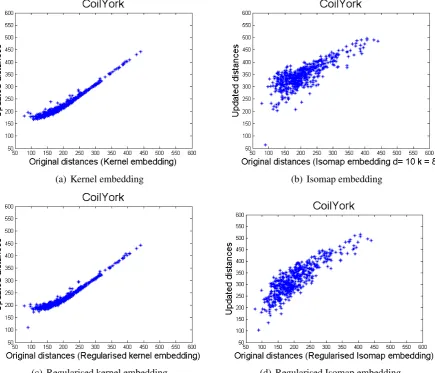
[image:25.595.78.507.112.303.2](a) Kernel embedding (b) Isomap embedding
[image:26.595.79.515.209.582.2](c) Regularised kernel embedding (d) Regularised Isomap embedding
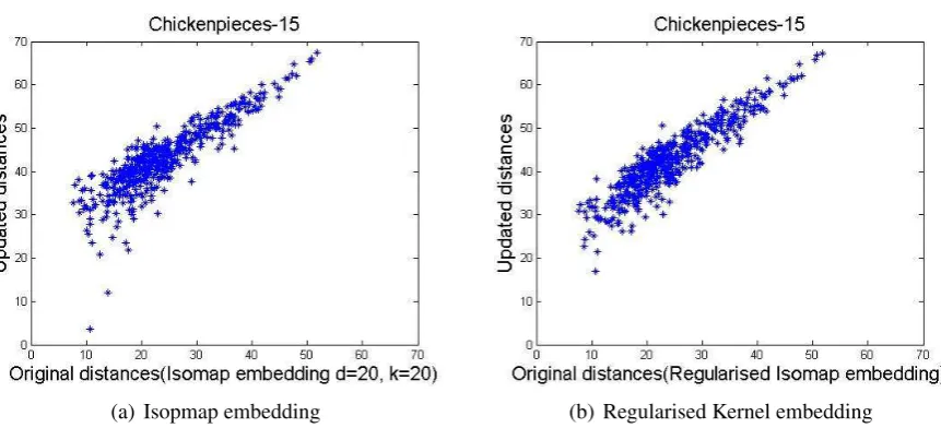
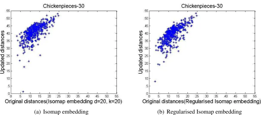
(a) Isomap embedding (b) Regularised Isomap embedding
Figure 7: (a) 500 random pairs of dissimilarities for the Chickenpieces-10 before and after 500 iterations of Ricci flow with Isomap embedding, (b) Regularised Ricci flow with Isomap embedding
(a) Isopmap embedding (b) Regularised Kernel embedding
[image:27.595.78.511.149.339.2] [image:27.595.80.511.460.656.2](a) Isomap embedding (b) Regularised Isomap embedding
Figure 9: (left) 500 random pairs of dissimilarities for the Chickenpieces-10 before and after 500 iterations of Ricci flow with Isomap embedding, (right) Regularised Ricci flow embedding with Isomap embedding
cases the updated dissimilarities depend approximately linearly on the initial dissimilarities. In the case of ISOMAP there is again more variance in the updated dissimilarities at a given input dissimilarities, and this is ascribable to the variance in curvature noted above.
Figure 6 extends this analysis to multiple iterations. Here we explore the effect of both the unregularised and regularised versions Ricci flow embedding on the kernel and IsoMap embed-dings. The figure shows plots of the updated Euclidean dissimilarities as a function of the original non-Euclidean dissimilarities after500iterations of Ricci flow. The left hand subfigures show the results obtained with kernel embedding while the righthand ones show the result of the Isomap embedding. The two plots in the top row are the result of Ricci flow while those in the lower row are the results of regularised Ricci flow.
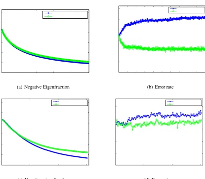
[image:28.595.76.513.106.299.2]0 50 100 150 200 250 300 350 400 450 500 0 0.0 5 0.1 0.1 5 0.2 0.2 5 0.3 0.3 5 It erat ionnumber(Ker nelembeddi ng) Negati veeigenf ract ion C oi lYor k R icc ifl ow R icc ifl
ow w it h regul
ari
zati
on
(a) Negative Eigenfraction
0 50 100 150 200 250 300 350 400 450 500
0 0.1 0.2 0.3 0.4 0.5 It erat ionnumber(Ker nelembeddi ng) Errorr ate C oi lYor k R ic cif low R ic cif loww it h regul ari zati on
(b) Error rate
0 50 100 150 200 250 300 350 400 450 500
0 0.0 5 0.1 0.1 5 0.2 0.2 5 0.3 0.3 5 It erat ionnumber(I
somap em beddi ng d=10,k=8) Negati veeigenf ract ion C oi lYor k R icc ifl ow R icc ifl
ow w it h regul
ari
zati
on
(c) Negative eigenfraction
0 100 200 300 400 500
0 0.0 5 0.1 0.1 5 0.2 0.2 5 0.3 0.3 5 0.4 0.4 5 It erat ionnumber(I
somap em beddi ng d=10,k=8) Errorr ate C oi lYor k R icc ifl ow R icc ifl
ow w it h regul
ari
zati
on
(d) Error rate
[image:29.595.90.512.212.587.2]0 100 200 300 400 500 0 0.0 5 0.1 0.1 5 0.2 0.2 5 0.3 It erat ionnumber(Ker nelembeddi ng) Negati veeigenf ract ion C hi ckenpi eces5 R icc ifl ow R icc ifl
ow w it h regul
ari
zati
on
(a) Negative Eigenfraction
0 50 100 150 200 250 300 350 400 450 500
0 0.1 0.2 0.3 0.4 0.5 0.6 It erat ionnumber(Ker nelembeddi ng) Errorr ate C hi ckenpi eces5 R icc ifl ow R icc ifl
ow w it h regul
ari
zati
on
(b) Error rate
0 50 100 150
0 0.0 5 0.1 0.1 5 0.2 0.2 5 0.3 It erat ionnumber(I
somap em beddi ng d=20,k=20) Negati veeigenf ract ion C hi ckenpi eces5 R icc ifl ow R icc ifl
ow w it h regul
ari
zati
on
(c) Negative eigenfraction
0 50 100 150
0 0.1 0.2 0.3 0.4 0.5 It erat ionnumber(I
somap em beddi ng d=20,k=20) Errorr ate C hi ckenpi eces5 R ic cif low R ic cif loww it h regul ari zati on
(d) Error rate
[image:30.595.91.507.207.570.2]0 50 100 150 0 0.0 5 0.1 0.1 5 0.2 0.2 5 0.3 0.3 5 0.4 It erat ionnumber(Ker nelembeddi ng) Negati veeigenf ract ion C hi ckenpi eces40 R icc ifl ow R icc ifl
ow w it h regul
ari
zati
on
(a) Negative Eigenfraction
0 50 100 150
0 0.0 5 0.1 0.1 5 0.2 0.2 5 0.3 0.3 5 0.4 It erat ionnumber(Ker nelembeddi ng) Errorr ate C hi ckenpi eces40 R ic cif low R ic cif loww it h regul ari zati on
(b) Error rate
0 10 20 30 40 50
0 0.0 5 0.1 0.1 5 0.2 0.2 5 0.3 0.3 5 0.4 It erat ionnumber(I
somap em beddi ng d=20,k=20) Negati veeigenf ract ion C hi ckenpi eces40 R icc ifl ow R icc ifl
ow w it h regul
ari
zati
on
(c) Negative eigenfraction
0 10 20 30 40 50
0 0.0 5 0.1 0.1 5 0.2 0.2 5 0.3 It erat ionnumber(I
somap em beddi ng d=20,k=20) Errorr ate C hi ckenpi eces40 R icc ifl ow R icc ifl
ow w it h regul
ari
zati
on
(d) Error rate
[image:31.595.91.507.202.581.2]Figure 13: Error rate from 1NN for chicken pieces dataset cost =45, (a) includes Ricci flow with Kernel embedding and Isomap embedding; (b) includes Ricci flow with regularised Kernel embedding and regularised Isomap embedding
i.e. (c) and (d).
Figures 7-9 repeat this analysis for the Isomap embedding on the Chickenpieces data with different edit parameters for the shape comparison process. The left-hand plot (a) shows the result of Ricci flow and the right-hand one (b) the result of regularised Ricci flow. As the edit parameter increases from 10 to 30 the variance of the dispersion of the Ricci flow plots increases, and the regularisation process appears to slightly reduce the final dispersion.
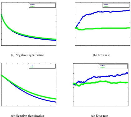
5.3. Iterative Performance
We now illustrate the iterative behavour of the two Ricci flow schemes on the COILYork data together with some of the Chickenpieces data. Fig. 10 show the results for the COILYork data, while Figs 11 and 12 and show two different examples for data withL = 5 andL = 40for the Chicenpieces data. In the top row of each figure the two subfigures show the negative eigenfraction (NEF) and error rate for Ricci flow on the kernel embedding as a function of iteration number, while the subfigures in the bottom row show the same quantities for Ricci flow applied to the Isomap embedding. In each plot the different curves compare piecewise and regularised Ricci flow. Since the convergence rate varies significantly for the different algorithms and datasets, the plots in Figures 11 and 12 have different scales along the horizontal axis.
with piecewise Ricci flow slightly outperforming regularised Ricci flow. In the case of Isomap the decrease is faster than with the kernel embedding. However, when we consider the 1-NN error, there is a marked difference in the behaviour of the piecewise and regularised Ricci flow methods. Only the regularised piecewise method is able to improve or maintain the level of 1-NN error, and the piecewise method disrupts it badly. So again see that the regularised Ricce flow method does well at rectifying the data, but has a tendency to disrupt structures present in the data.
We have compared our classification results with those obtained with Isomap, together with those obtained with using just the positive subspace and those obtained with the original dissimi-larities. Figure 13 (b) shows the 1NN error rate as function of the shape parameterL(the segment length). The best results are obtained with the regularized Ricci flow on kernel embedding. Figure 13 (a) shows that the unregularised version of Ricci flow embedding when used with both em-bedding schemes gives poorer results than when the Isomap emem-bedding alone is used. Hence we conclude that the regularized Ricci flow embedding performs better than the unregularised version (the results of the unregularised version are not repeated here). All of the remaining methods give poorer results than simply applying the classifier to the original dissimilarity data. Our regularised Ricci flow embedding is therefore shown to be a potentially good way to perform Euclidean rectifi-cation on the non-Euclidean dissimilarity data. The discriminating power of the rectified Euclidean dissimilarity is close to that of the original non-Euclidean dissimilarities.
Finally, we provide some time complexity considerations for our method. These are based on one iteration of our method, and the overall complexity will of course depend and the speed of convergence and number of iterations used. The time complexity for both Isomap and kernel em-bedding is approximatelyO(dn2)[27], wheredis the output dimensionality andn is the number of data points. To compute the curvatures for the edges and the geometric updating are bothO(n2). In the regularised version of the algorithm there is the additional step of heat kernel smoothing. Computing the heat kernel is O(k3n3) since it depends on the eigen-decomposition of the dual neighbourhood graph Laplacian which is cubic in the number of nodes in the dual graph, i.e. kn. Convolving the heat kernel with the nodes of the graph isO(k2n2). Assume each local patch has
k points and there are m patches, so the limiting time complexity of the regularised version is
5.4. Classification Experiments
To evaluate the quality of the rectified Euclidean dissimilarities, we explore their use in classi-fication experiments. The experiments were performed to determine whether the Ricci evolution preserves the class structure in data. We compared the results obtained with the different variants of our Ricci flow algorithm, with those obtained using a number of alternative Euclidean correc-tion procedures. The methods studied were a) spectrum clip, b) spectrum flip c), spectrum shift and d) Isomap embedding.
Table 1 reports the results obtained by applying five different classifiers to the corrected Eu-clidean dissimilarities obtained using ten different rectification methods. The data used was taken from the Chickenpieces, CoilYork and Yeast-SW-7-12 datasets. The first point to note is that spec-trum clip causes a deterioration of the results obtained by nearest neighbour classifiers. However, spectrum clip achieves best performance when used in conjunction with SVM on the Chicken-pieces data (ChickenChicken-pieces-10, ChickenChicken-pieces-15, ChickenChicken-pieces-20 and ChickenChicken-pieces-25). It destroys local dissimilarities but preserves global dissimilarities. Similarly spectrum flip destroys the local structure of the data. Spectrum shift preserves the ranking of dissimilarity values, and so the nearest neighbour classifier performance on the resulting corrected Euclidean dissimilarity is identical to that obtained on the original uncorrected dissimilarity data. The Isomap embed-ding gives better performance than both spectrum clip and spectrum flip for nearest neighbour classifiers.
kernel embedding, Ricci flow destroys the local structure of the hyperbolic patches in the data. This also explains why the results from the Ricci flow with the Isomap embedding are worse than those from the pure Isomap embedding. Since the curvature increases much more rapidly for shorter dissimilarities in the kernel embedding, the change in dissimilarity induced by Ricci flow is rapid and potentially unstable.
Because of this instability when Ricci flow is unregularised, we turn our attention to the per-formance of the regularised version of our Ricci flow embedding procedure. The first point to note is that for both the kernel embedding and the Isomap embedding methods, we obtain better classi-fication results when heat kernel regularisation is used in conjunction with Ricci flow. Regularised Ricci flow with Isomap embedding gives better performance than regularised Ricci flow with ker-nel embedding. Overall the best results are obtained using the regularized Ricci flow with Isomap embedding. This is the case for most of the datasets, when both nearest neighbour classifiers and SVMs are applied to the corrected data. All of the remaining methods give results that are worse than applying the nearest classifier to the original dissimilarity data. So we conclude that when applied to ISOMAP, our regularised Ricci flow algorithm is a potentially good way to rectify the non-Euclidean dissimilarity data since it appears to best preserve the local structure residing in the original non-Euclidean dissimilarities.
Chickenpieces-5 (NEF =21.6%)
Original Clip Flip Shift Isomap RFK RRFK RFI RRFI
1NN 34.53 46.19 49.10 34.53 38.34 50.67 21.30 43.05 36.10 3NN 34.53 44.39 47.98 34.53 39.01 50.90 26.46 43.50 33.63 5NN 36.77 43.95 50.00 36.77 39.46 53.59 36.55 44.39 33.18
Linear SVM 19.06 21.75 22.42 21.75 24.44 17.71 32.74 18.83 RBF SVM 19.06 21.30 23.09 19.73 23.32 15.92 32.51 15.92
Chickenpieces-10 (NEF =25.7%)
Original Clip Flip Shift Isomap RFK RRFK RFI RRFI
1NN 16.14 34.53 44.39 16.14 22.42 49.78 11.66 34.75 17.26 3NN 19.06 36.10 48.21 19.06 20.63 51.35 21.30 34.30 14.80
5NN 23.32 38.12 48.21 23.32 21.30 54.04 34.08 32.74 15.47
Linear SVM 8.07 9.86 12.11 21.07 12.10 9.64 21.52 14.13 RBF SVM 6.50 8.97 12.11 16.59 11.65 8.52 21.30 14.35
Chickenpieces-15 (NEF =28.6%)
Original Clip Flip Shift Isomap RFK RRFK RFI RRFI
1NN 7.40 23.99 43.72 7.40 12.78 47.76 4.48 23.32 4.93 3NN 8.30 28.48 41.70 8.30 11.88 47.09 13.90 21.52 5.61
5NN 11.43 31.39 43.95 11.43 12.33 49.55 27.80 21.30 8.07
Linear SVM 4.48 6.73 12.11 12.11 10.09 7.17 12.33 12.33 RBF SVM 4.26 6.95 14.13 10.99 8.97 5.38 12.78 12.56
Chickenpieces-20 (NEF =30.7%)
Original Clip Flip Shift Isomap RFK RRFK RFI RRFI
1NN 6.28 17.04 36.55 6.28 9.87 42.38 4.93 21.52 4.48
3NN 9.64 21.75 38.79 9.64 10.31 45.52 15.25 19.51 5.61
5NN 10.31 21.97 41.70 10.31 10.99 47.09 30.04 19.28 6.28
Chickenpieces-25 (NEF =31.99%)
Original Clip Flip Shift Isomap RFK RRFK RFI RRFI
1NN 4.26 14.13 32.96 4.26 8.74 40.36 4.93 17.49 5.38 3NN 7.62 15.70 34.30 7.62 9.19 39.91 15.02 21.08 6.73
5NN 7.17 19.06 35.20 7.17 9.64 42.38 25.34 19.73 8.30 Linear SVM 2.90 4.26 7.40 8.52 7.84 5.60 11.66 6.73 RBF SVM 2.69 5.38 7.40 10.54 4.93 8.74 9.87 5.16
Chickenpieces-30 (NEF =33.07%)
Original Clip Flip Shift Isomap RFK RRFK RFI RRFI
1NN 4.48 13.00 30.49 4.48 5.83 37.67 5.83 15.47 4.71 3NN 4.48 14.80 32.74 4.48 6.05 41.93 13.68 19.06 4.93 5NN 5.38 15.70 34.75 5.38 7.40 41.93 26.68 18.61 5.16
Linear SVM 4.48 5.16 6.95 7.17 9.64 9.87 10.54 4.03
RBF SVM 5.61 5.16 6.95 4.930 8.29 7.85 10.31 3.13
Chickenpieces-35 (NEF =33.94%)
Original Clip Flip Shift Isomap RFK RRFK RFI RRFI
1NN 6.28 15.02 31.84 6.28 7.17 39.69 6.50 16.82 4.93
3NN 5.38 17.94 36.10 5.38 8.52 43.50 14.35 19.51 4.71
5NN 6.05 19.28 37.22 6.05 9.64 44.84 25.34 18.39 5.61
Linear SVM 6.73 6.95 7.62 6.50 9.19 5.83 7.85 4.26
RBF SVM 6.95 6.50 7.62 5.830 7.62 5.61 7.85 3.59
Chickenpieces-40 (NEF =34.46%)
Original Clip Flip Shift Isomap RFK RRFK RFI RRFI
1NN 8.74 15.25 28.03 8.74 9.64 35.20 8.74 19.28 6.95
3NN 8.52 15.70 32.29 8.52 11.21 35.87 17.71 20.40 7.62
5NN 9.19 16.59 34.30 9.19 12.11 37.00 25.34 19.73 8.97
Linear SVM 6.73 7.85 9.87 10.76 11.21 8.52 11.66 5.16
CoilYork (NEF =25.76%)
Original Clip Flip Shift Isomap RFK RRFK RFI RRFI
1NN 23.26 33.68 50.35 23.96 44.44 47.92 24.13 36.57 25.86 3NN 29.17 34.38 46.53 29.86 42.36 44.79 28.12 35.76 27.78
5NN 27.08 35.42 45.49 28.12 39.24 45.49 33.68 32.64 25.69
Linear SVM 37.15 40.97 35.42 42.01 45.48 42.36 30.90 26.39
RBF SVM 31.59 36.11 33.68 33.68 37.15 31.25 27.08 21.53
Yeast-SW-7-12 (NEF =42.57%)
Original Clip Flip Shift Isomap RFK RRFK RFI RRFI
1NN 10.50 19.00 26.00 10.50 10.50 14.00 15.00 15.00 9.00
3NN 14.50 21.00 31.50 16.00 16.50 13.50 14.50 14.50 11.00
5NN 14.00 20.00 31.50 14.50 17.00 13.00 13.00 14.50 13.00
Linear SVM 8.5 9.0 10.0 31.5 7.5 7.5 7.5 8.00
[image:38.595.67.489.109.378.2]RBF SVM 8.5 9.0 10.0 11.5 8.5 9.0 8.5 7.00
Table 1: Clip, flip, shift, Isomap, Ricci flow with kernel embedding (RFK), regularised Ricci flow with kernel embedding (RRFK), Ricci flow with Isomap embedding(RFI) and regularised Ricci flow with Isomap embedding(RRFI) comparison. Table shows % misclassifications of the nearest classifiers including 1NN, 3NN and 5NN using leave one out cross validation, of the linear SVM and RBF SVM over ten fold cross validation.
6. Conclusions
In this paper, we have explored how to rectify non-Euclidean dissimilarity data by using Ricci flow to flatten the embedding of the data. We have presented two variants of the Ricci flow al-gorithm, the first is piecewise and unregularised while the second uses curvature regularisation. We have compared these variants of our algorithm with spectrum clipping, flipping and shifting on a variety of real world data. These experiments show that the piecewise Ricci flow embedding is rather unstable while the regularized Ricci flow embedding is able to effectively rectify non-Euclidean dissimilarities. In particular, the regularised Ricci flow method preserves local struc-tures present in the data, which proves useful for classification. Piecewise unregularised Ricci flow, proves too unstable to be useful on its own.
extended. First, it would be interesting to establish convergence properties, and in particular how the negative eigenvalues of the dissimilarities behave under the Ricci flow. Unfortunately this has proved intractable. The reasons for this are twofold. Firstly, the iterative methods for updating the dissimilarities involve quite complex inverse-trigonometrical relations, and these are difficult to analyse. Secondly, the Euclidean dissimilarities used are determined by the previously computed geodesic dissimilarities and the embedding methods used, i.e. Isomap or kernel embedding. Thus understanding the dissimilarity sequences is also not straightforward. Moreover, computing the negative eigenvalues involves solving the eigensystem for the dissimilarity matrix.
Our second line of future work will be to explore more applications of the method. Although our Chickenpieces application involves shape analysis, it is not formally posed in terms of the con-struction of shape spaces. Many problems in shape analysis involve non-Euclidean dissimilarities and it would be interesting to see if our method can lead to better structured shape spaces. Another area where the method can be of use is in structural pattern recognition, where graph edit dissim-ilarities also show non-Euclidean properties, and our methods may lead to better graph clustering results. Finally, it would be interesting to investigate whether our method can be rendered more efficient through sparsification.
[1] I. Biederman. Recognition-by-components: A theory of human image understanding. Psychological Review,
94(2):115–147, 1987.
[2] C. M. Bishop. Neural networks for pattern recognition. Oxford University Press, USA, 1995.
[3] H. Bunke and A.Sanfeliu. Syntactic and Structural Pattern Recognition: Theory and Applications. World
Scientific, 1990.
[4] B. Chow and F. Luo. Combinatorial Ricci flows on surfaces. J. Differential Geom, 63(1):97–129, 2003.
[5] F.R.K. Chung.Spectral graph theory. American Mathematical Society, 1996.
[6] M.P. Dubuisson and A.K. Jain. A modified Hausdorff distance for object matching. In IAPR International
Conference on Pattern Recognition, volume 1, 1994.
[7] R.O. Duda, P.E. Hart, and D.G. Stork. Pattern classification. Wiley New York, 2001.
[8] R.P.W. Duin and E. Pekalska. Non-Euclidean dissimilarities : causes and informativeness. SSPR/SPR 2010,
pages 324–333, 2009.
[9] R.P.W. Duin, E. Pekalska, A. Harol, W-J. Lee, and H. Bunke. On Euclidean corrections for Non-Euclidean
dissimilarities. InSSPR/SPR, pages 551–561, 2008.
Approx. Reasoning, 50(2):363–384, 2009.
[11] S. Gold and A. Rangarajan. A graduated assignment algorithm for graph matching. IEEE Transactions on
Pattern Analysis and Machine Intelligence, 18:377–388, 1996.
[12] J.C. Gower. Properties of euclidean and non-euclidean distance matrices. Linear Algebra and its Applications,
67:81–97, 1985.
[13] J.C. Gower and P. Legendre. Metric and Euclidean properties of dissimilarity coefficients. Journal of
Classifi-cation, 3(1):5–48, 1986.
[14] X. Gu, Y. He, M. Jin, F. Luo, H. Qin, and S.T. Yau. Manifold splines with a single extraordinary point.
Computer-Aided Design, 40(6):676–690, 2008.
[15] B. Haasdonk and E. Pekalska. Indefinite kernel fisher discriminant. InProc. of ICPR 2008, International
Conference on Pattern Recognition, 2008.
[16] R.S. Hamilton. Three-manifolds with positive Ricci curvature.J. Differential Geom, 17(2):255–306, 1982.
[17] R.S. Hamilton. The ricci flow on surfaces.Contemp. Math, 71:237–262, 1988.
[18] X. Jiang and X. Gu. Multiscale, curvature-based shape representation for surfaces.International Conference on
Computer Vision (ICCV), pages 1887–1894, 2011.
[19] M. Jin, J. Kim, and X. Gu. Discrete surface ricci flow: Theory and applications. Mathematics of Surfaces XII,
pages 209–232, 2007.
[20] M. Jin, F. Luo, and X. Gu. Computing surface hyperbolic structure and real projective structure.Proceedings of
the 2006 ACM symposium on Solid and physical modeling, pages 105–116, 2006.
[21] R.I. Kondor and J. Lafferty. Diffusion kernels on graphs and other discrete structures. InProceedings of the
ICML, pages 315–322, 2002.
[22] G. R. G. Lanckriet, M. Deng, N. Cristianini, M. I. Jordan, and W. S. Noble. Kernel-based data fusion and its
application to protein function prediction in yeast. InProceedings of the Pacific Symposium on Biocomputing,
2004.
[23] J. Laub.Non-metric pairwise proximity data. PhD thesis, Berlin Institute of Technology, 10, Dec 2004.
[24] J. Laub, V. Roth, J.M. Buhmann, and K.R. M¨uller. On the information and representation of Non-Euclidean
pairwise data. Pattern Recognition, 39(10):1815–1826, 2006.
[25] Harold Lindman and Terry Caelli. Constant curvature Riemannian scaling.Journal of Mathematical Psychology,
17:89–109, 1978.
[26] T. Mitchell.Machine learning. McGraw-Hill, 1997.
[27] F. Pedregosa, G. Varoquaux, A. Gramfort, V. Michel, B. Thirion, O. Grisel, M. Blondel, P. Prettenhofer,
R. Weiss, V. Dubourg, J. Vanderplas, A. Passos, D. Cournapeau, M. Brucher, M. Perrot, and E. Duchesnay.
Scikit-learn: Machine learning in Python. Journal of Machine Learning Research, 12:2825–2830, 2011.
Ap-plications. World Scientific Publishing Co Pte Ltd, 2005.
[29] E. Pekalska and R.P.W. Duin. Beyond traditional kernels: classification in two dissimilarity-based representation
spaces. IEEE Transactions on Systems, Man and Cybernetics–Part C, 38(6), November 2008.
[30] E. Pekalska, R.P.W. Duin, S. Gunter, and H. Bunke. On not making dissimilarities Euclidean. Lecture notes in
computer science, pages 1145–1154, 2004.
[31] E. Pekalska, A. Harol, R. Duin, B. Spillmann, and H. Bunke. Non-Euclidean or non-metric measures can be
informative. Structural, Syntactic, and Statistical Pattern Recognition, pages 871–880, 2006.
[32] E. Pekalska, P. Paclik, and R.P.W. Duin. A generalized kernel approach to dissimilarity-based classification. J.
Mach. Learn. Res., 2:175–211, 2001.
[33] G. Perelman, G. Perelman, and G. Perelman. Finite extinction time for the solutions to the ricci flow on certain
three-manifolds. PLoS Biology, 4(5):e8, 2006.
[34] D. Poole.Linear algebra: a modern introduction. Cengage Learning, 2005.
[35] A. Robles-Kelly and E.R. Hancock. A Riemannian approach to graph embedding. Pattern Recognition,
40(3):1042–1056, 2007.
[36] V. Roth, J. Laub, J.M. Buhmann, and K.R. M¨uller. Going metric: Denoising pairwise data.Advances in Neural
Information Processing Systems, 15:817–824, 2002.
[37] A. Sanfeliu and K. S. Fu. A distance measure between attributed relational graphs for pattern recognition.IEEE
Transactions on Systems, Man, and Cybernetics, 13(3):353–362, 1983.
[38] R. Sarkar, X. Yin, J. Gao, F. Luo, and X.D. Gu. Greedy routing with guaranteed delivery using ricci flows.
International Conference on Information Processing in Sensor Networks, pages 121–132, 2009.
[39] E. Saucan, E. Appleboim, E.G. Wolansky, and Y.Y. Zeevi. Combinatorial ricci curvature and Laplacians for
image processing. CISR, 2009.
[40] L. G. Shapiro and R. M. Haralick. A metric for comparing relational descriptions.IEEE Transactions on Pattern
Analysis and Machine Intelligence, 7(1):90–94, 1985.
[41] T. Tao. Ricci flow. Technical report, Department of Mathematics, UCLA, 2008.
[42] J.B. Tenenbaum, V. Silva, and J.C. Langford. A global geometric framework for nonlinear dimensionality
reduction. Science, 290:2319–2323, 2000.
[43] World Scientific Publishing Company.Riemannian manifolds of positive curvature, 2011.
[44] B. Xiao and E. R. Hancock. Geometric characterisation of graphs. ICIAP, LNCS 3617:471–478, 2005.
[45] B. Xiao, E.R. Hancock, and R.C. Wilson. Geometric characterization and clustering of graphs using heat kernel
embeddings. Image and Vision Computing, 28(6):1003–1021, 2010.
[46] Wilson R. C. & Hancock E. R. Xiao, B. Characterising graphs using the heat kernel.BMVC, 2005.
[47] W. Xu, E. R. Hancock, and R. C. Wilson. Regularising the ricci flow embedding. InSSPR/SPR, pages 579–588,
[48] W. Xu, E.R. Hancock, and R. C. Wilson. Rectifying non-euclidean similarity data using ricci flow embedding.
2010.
[49] W. Zeng, D. Samaras, and D. Gu. Ricci flow for 3d shape analysis.IEEE Transactions on Pattern Analysis and
Machine Intelligence, 32(4):662–677, 2010.
[50] W. Zeng, X. Yin, Y. Zeng, Y. Lai, X. Gu, and D. Samaras. 3d face matching and registration based on
hyper-bolic ricci flow. IEEE Computer Society Conference on Computer Vision and Pattern Recognition Workshops