Genetic Algorithm Based Routing Technique to Extend Lifetime of Wireless Sensor Network

International

 

Journal

 

of

 

Advanced

 

Research

 

in

 

Computer

 

Science

 

RESEARCH

 

PAPER

 

Available Online at www.ijarcs.info 

Genetic Algorithm Based Routing Technique to Extend Lifetime of Wireless Sensor

Network

Mr. Keyur M. Rana*

Department of Computer Engineering Sarvajanik college of Engineering & Technology

Surat, India. [email protected]

Dr. Mukesh A. Zaveri

Department of Computer Engineering Sardar Vallabhbhai National Institute of Technology

Surat, India [email protected]

Abstract: Various routing protocols have been designed and developed for Wireless Sensor Networks. They face various challenges. Sensor

nodes are strongly energy and storage constrained and failure rate of sensor node is very high. While sending data to the sink node, some routing mechanisms which consider all these parameters, are needed to extend life of the network. There are several techniques for routing in wireless sensor network for data gathering using aggregation and for data gathering using without aggregation. Researchers have suggested Genetic Al-gorithm (GA) based approach for extending life of wireless sensor network for data gathering with aggregation. We have proposed modified GA based approach which takes into account, data gathering without aggregation. We have used a pre-defined minimum energy level (Level1) for sensor nodes so, that they don’t participate in routing if their residual energy level is below this level and other better path is still available. If there exist no such path, then this node can be part of routing. We have also experimented for optimal value of energy level, Level1.

Keywords: Wireless sensor network; Routing; Genetic Algorithm

I. INTRODUCTION

In wireless sensor network (WSN), each sensor is battery operated. We assume that batteries are neither replaceable nor rechargeable. This is the case when the sensors are deployed in hostile environment or in a kind of environments where it is hard to reach. Sensor nodes are capable of performing some processing, gathering sensory information such as monitoring physical phenomena like temperature, humidity, vibrations and communicating with other neighbor nodes [1]. In many appli-cations, lifetime of network requires several months or even years. The sensor network should be capable enough to fulfill the application requirements. How to prolong network lifetime to such a long time is the vital question.

Generally in routing algorithm, the best path is chosen for transmission of data from source to destination. Over the period of time, if same path is chosen for communication in order to achieve better performance in terms of quick transmission time, then those nodes which are on this path may get drained earlier. The problem with these protocols is that they minimize the total energy consumed in the network, but drain energy along paths chosen for minimum energy consumption. This approach causes network partition because some node which are part of the efficient path, are drained from their battery energy quicker. When these nodes get exhausted, they may break network into parts because of unavailability of other path. In many cases, the lifetime of a sensor network is over as soon as the battery pow-er in critical nodes is depleted [2]. Thpow-ere are sevpow-eral challenges in wireless sensor network. Sensor nodes are tightly con-strained in terms of energy, processing, and storage capacities, so they require careful resource management. As node failure is occurred frequently in WSNs which results in unpredictable and frequent topological changes. Therefore, the routing proto-col must adapt to frequent changes of the WSNs topology.

Some special nodes, called relay nodes can also be used within the network, for balanced data gathering to extend life of network. In case of hierarchical sensor network, cluster head is

called as relay node. These relay nodes are set with higher en-ergy as compared to the sensor nodes.

A Genetic Algorithm (GA) based approach for energy effi-cient routing has been proposed by Ataul Bari et. al [3]. They have suggested this approach for two-tiered sensor network. They have given solution for data gathering with aggregation. We have proposed a new GA based approach for data gathering without aggregation. We have used total energy consumed and total number of nodes below a pre-defined level (Level1) of minimum energy, as criteria to choose route and the same has been used as fitness function of proposed genetic algorithm based approach.

To find best path, Warshall’s algorithm [4, 5] can be used. Warshall’s algorithm compares all possible paths through the graph between each pair of vertices. This algorithm has also been used and simulated. Result of simulations are compared for Warshall’s algorithm, GA based approach [3] and proposed GA based approach.

II. ROUTING IN WSN

A routing protocol is required when a source node cannot send its packets directly to its destination node but has to rely on the assistance of intermediate nodes to forward these pack-ets on its behalf.

Routing protocols can be divided into two groups, proactive and reactive routing protocols [6]. With proactive routing a routing table is generated at each node, so that routing informa-tion is kept for every node in the network. This is used in tradi-tional link-state and distance vector routing protocols, with the DSDV (Destination-Sequenced Distance Vector) protocol be-ing proposed for wireless sensor networks.

With reactive routing no routing tables are generated and route discovery is done as needed. The route information is then kept for future reference. Existing reactive protocols in-clude AODV (Ad hoc On-demand Distance Vector) and DSR (Dynamic Source Routing).

The problem with these protocols is that they minimize the total energy consumed in the network, but drain energy along paths chosen for minimum energy consumption. This approach causes network partition because some node which are part of the efficient path, are drained from their battery energy quicker. When these nodes get exhausted, they may break network in to parts because of unavailability of other path.

Many researchers have proposed the use of some special nodes, called relay nodes within the network, for balanced data gathering to extend life of network. In case of hierarchical sen-sor network, relay nodes can be used as cluster head. These cluster heads are equipped with higher energy as compared to the sensor nodes.

[image:2.595.37.285.361.522.2]

In this paper we will be refereeing mainly to the sensor network model depicted in Fig. 1.

Figure 1. An example of a two-tiered (hierarchical) sensor network [3]

This figure shows that sensor network is divided in cluster and each cluster contains one relay node and many sensor nodes. There is also one Base station where information is for-warded by sensor nodes via relay nodes. Each relay node can communicate either with other relay nodes or to the Base sta-tion. Sensor nodes can communicate with relay nodes of their cluster. Clustering strategies for this model can be referred from [7].

It has been seen that generally data transmission is very ex-pensive in terms of energy consumption while data processing consumes comparatively less energy. The ratio of the energy cost of transmitting a single bit of information to the energy needed for processing a thousand operations in a typical sensor node is 1:1000 [8].

The lifetime of a sensor network can be extended by apply-ing different techniques [9] .

III. GENETIC ALGORITHM BASED APPROACH

Researchers have proposed the use of some special nodes, called relay nodes [3, 10] within the network, for balanced data gathering, to achieve fault tolerance and to extend network

life-time. The relay nodes can be used as cluster heads in hierarchi-cal sensor networks and can be provisioned with higher energy as compared to the sensor nodes.

In a two-tiered network architecture, where higher powered relay nodes act as cluster heads and sensor nodes transmit their data directly to their respective cluster heads. However, the relay nodes are still battery operated and hence, power con-strained. Total depletion of the power of a relay node severely impacts the functionality of the network, since all sensor nodes belonging to the cluster of the depleted relay node will be un-able to send their data to the base station and the entire cluster becomes inoperative. This may also put additional load on the surviving relay nodes and will cause faster depletion of the batteries of other relay nodes. Fig. 1 shows example of a two tiered sensor network.

In this model, the lifetime of a network is determined main-ly by the lifetimes of these relay nodes. An energy-aware communication approach can greatly extend the lifetime of such networks. However, integer linear program (ILP) formula-tions for optimal, energy-aware routing quickly become com-putationally intractable and are not suitable for practical net-works. In [3], Atul Bari et al., have proposed a solution, based on a genetic algorithm (GA), for scheduling the data gathering of relay nodes. This efficient solution can significantly extend the lifetime of a relay node network. This algorithm can easily handle large networks, where it leads to significant improve-ments compared to traditional routing schemes.

A. Genetic Algorithm Overview

Genetic algorithm (GA) is modeled after the natural process of evolution as it occurs through offspring. For most genetic algorithms, the main concept is that the strongest individuals survive a generation (survival of the fittest) and reproduce with other survivors, producing (hopefully) an even stronger child [11]. The Genetic Algorithm is a technique for randomized search and optimization and has been applied in a wide range of studies in solving optimization problems, especially prob-lems that are not well structured and interact with large num-bers of possible solutions. In GA the search space of a problem is represented as a collection of individuals.

The individuals are represented by character strings, which are often referred to as chromosomes. The GA starts with the set of the randomly generated possible solutions. Each solution is a chromosome. The length of the each chromosome in the population should be the same. The purpose of the use of a GA is to find the individual from the search space with the best ''genetic material.'' The quality of an individual is measured with an objective function called as fitness function. A fitness function is provided to assign the fitness value for each indi-vidual. This function is based on how close an individual is to the optimal solution – the higher the fitness value, the closer is the solution to the optimal solution.

Algorithm 1: Genetic Algorithm

begin

Generate an initial population

Compute the fitness of each individual while (not stopping criterion) do

Choose parents from population. Perform crossover to produce offsprings. Perform mutations.

Compute fitness of each individual.

Replace the parents by the corresponding offsprings in new generation.

Two randomly selected chromosomes, known as parents, can exchange genetic information in a process called recombi-nation or crossover, to produce two new chromosomes known as child or offspring. If both the parents share a particular pat-tern in their chromosome, then the same patpat-tern will be carried over to the off springs. To obtain a good solution, mutation is often applied on randomly chosen chromosomes, after the process of crossover. Mutation helps to restore any lost genetic values when the population converges too fast. Once the proc-esses of crossover and mutation have occurred in a population, the chromosomes for the next generation are selected. To en-sure that the new generation is at least as fit as the previous generation, some of the poorest performing individuals of the current generation can be replaced by the same number of the best performing individuals from the previous generation. For example, say, best 10% individuals are copied as it is in the next generation, which will replace the equal amount of the poorest individuals. This process is called elitism. This entire cycle is repeated until the stopping criterion of the algorithm is met. The steps of a standard GA [12] are outlined in Algorithm 1.

B. Wireless Sensor Network Model

For this model, a two-tiered wireless sensor network has been considered, with n relay nodes (acting as cluster heads). They are labeled as node numbers 1, 2, 3, . . . , n and one base station, labeled as node number n+1. This labeling is done for representing the network in form of chromosome in genetic algorithm. Let D be the set of all sensor nodes, and Di, 1≤ i ≤ n, be the set of sensor nodes belonging to the ith _{cluster, which has} relay node i as its cluster head. We assume that each sensor node belongs to exactly one cluster

i.e., D =D1

∪

D2

∪

. . .

∪

Dn and Di

∩

Dj =Φ for i≠j. A number of different metrics have been used in the litera-ture to measure the lifetime of a sensor network. In [13], the lifetime of a sensor network has been defined as the minimum of (i) the time when the percentage of nodes that are alive (i.e., nodes whose batteries are not depleted) drops below a specified threshold, (ii) the time when the size of the largest connected component of the network drops below a specified threshold, and (iii) the time when the volume covered drops below a spe-cified threshold. The work of [14] has defined the lifetime of the network as the lifetime of the sensor node that dies first. In [15], a number of metrics are used to define the network life-time, e.g., N-of-N lifetime (i.e., time till any relay/gateway node dies), K-of-N lifetime (i.e., time till, a minimum of K re-lay/gateway nodes are alive) and m-in-K-of-N lifetime (i.e., time till, all m supporting nodes and overall a minimum of K relay/gateway nodes are alive). In this approach of routing us-ing GA, N-of-N lifetime has been used. However, it can be used with other metrics by simply modifying the way the fit-ness of a chromosome is calculated.

C. Genetic Algorithm based Routing

Given a collection of n relay nodes, numbered from 1 to n, and a base station, numbered as n+1, along with their locations, the objective of the GA is to find a schedule for data gathering in a sensor network, such that the lifetime of the network is maximized. Each period of data gathering is referred to as a round [10], and the lifetime is measured by the number of rounds until the first relay node runs out of power. In other words, the N-of-N metric is used to measure the network life-time. It is also assumed that the initial energy provisioned in each relay node is equal.

Our routing model satisfies the following characteristics, which can be used to design initial population of genetic algo-rithm.

• Each relay node receives data from the sensor nodes belonging to its own cluster, and can also receive data from any number of other relay nodes.

• Each relay node i transmits data to one other node j (ei-ther ano(ei-ther relay node or the base station), such that node j is within the transmission range of node i and j is either the base station, or j is a relay node that is closer to the base station than node i.

• The base station only receives data, there is no trans-mission from base station to any relay node.

[image:3.595.306.557.308.437.2]

Now, the chromosome representation is defined, specify the initial population, describe the fitness function, and the strate-gies for crossover and mutation. The chromosome is repre-sented, for a specific routing scheme, as a string of node num-bers. The length of each chromosome is always equal to the number of relay nodes. A routing scheme for a network with 6 relay nodes, and one base station, is shown in Fig. 2 (a) and the corresponding chromosome is shown in Fig. 2 (b). In this ex-ample, the value of the gene in position 1 is 3, indicating that node 1 transmits to node 3. Similarly, the value in position 3 is 7, indicating that node 3 transmits to node 7 (base station).

Figure 2. Representation of network graph as chromosome [3]

1) Initial Population and Fitness Function:

Each chromosome in the initial population corresponds to a valid routing scheme. In our approach, the construction of this initial routing is based on the positions of the relay nodes, which is used by the base station to first create a list, Ni, 1≤ i ≤ n, that contains all the one-hop neighbors j, of i, such that the link i → j,

∀

j

∈

Ni can be used to route data from i towards the destination (base station) through j. For example, node 1, from Fig .2, will have Ni (where i=1) ={2, 3, 5} which are one hop neighbor of node 1. These are the nodes (referred as j) who leads i towards the destination. Here node 1 can reach to node 7 (destination) through node 2, 3 or 5 only. Based on this infor-mation, possible routing schemes i.e. chromosomes, for the initial population are generated using a greedy approach, by randomly picking up the next hop node j

∈

Ni for each source node i.

The search space for this problem is enormous. On an aver-age, if each node has d valid one-hop neighbors, then the num-ber of feasible routings for a network with n nodes is O(dn_{). In}

order to select a ‘‘good” energy efficient routing scheme, from such a large number of possible solutions, within a reasonable amount of time, a heuristic search technique, such as GA, is needed.

max

E E

L initial

net=

where Lnet is the network lifetime in terms of rounds and Einitial is the initial energy of a relay node. We assume that the value of Einitial is known beforehand and is the same for all relay nodes. Emax is the maximum energy dissipated by any relay node in the individual in one round of data collection.

It is assumed that Einitial is known initially and will remain same. But Emax is the maximum power dissipated by any node of the chromosome. E.g. in Fig. 2(b), maximum energy dissi-pated from node 1 to 3, form node 2 to 4, from node 3 to 7, from node 4 to 7, from node 5 to 3 and from node 6 to 7 is considered as Emax.

i.e. Emax = Max Energy Dissipated from node (1 to 3, 2 to 4, 3

to 7, 4 to 7, 5 to 3, 6 to 7)

Such fitness calculation is done for each individual of the population.

2) Selection and Crossover

Selection of individuals is carried out using the Roulette-Wheel selection method [16]. As per this method, those indi-viduals having higher fitness value will have higher probability to get selected.

To produce new offspring from the selected parents, the uniform crossover or k-point crossover (k = 1, 2, or 3, selected randomly) can be used for each crossover operation [3].

3) Mutation

Selection and crossover alone can obviously generate an amazing amount of differing strings. However, depending on the initial population chosen, there may not be enough variety of strings to ensure the genetic algorithm sees the entire prob-lem space. Or the GA may find itself converging on strings that are not quite close to the optimum it seeks due to a bad initial population.

Some of these problems are overcome by introducing a mu-tation operator into the GA. For each string element in each string in the mating pool, the GA checks to see if it should per-form a mutation. If it should, it randomly changes the element value to a new one. In the binary strings, 1s are changed to 0s and 0s to 1s. If it is not binary encoding of chromosome, then it should change as per the encoding is validated.

The mutation probability should be kept very low as a high mutation rate will destroy fit strings and deteriorate the GA algorithm into a random walk, with all the associated problems. But mutation will help prevent the population from having same value and become unused. Remember that much of the power of a genetic algorithm comes from the fact that it con-tains a rich set of strings of great diversity. Mutation helps to maintain that diversity throughout the genetic algorithm's itera-tions.

Mutation is usually applied after the process of crossover, to improve the fitness value of an individual. To perform the mutation over an individual for this problem, instead of ran-domly selecting a gene, as in standard GA, the node selected, say node i, is the one which dissipates the maximum energy due to the receiving and/or transmitting of its data. Node i is denoted as the critical node as it decides the lifetime of the network. The purpose of selecting node i for mutation is to reduce the total energy dissipation by the node and hence, to increase the network lifetime.

IV. PROPOSED ALGORITHM USING GA APPROACH

As in [3, 10], we have considered two tired network having m sensor nodes. Entire network is divided in different clusters and each cluster head is considered as a relay node. There are

such, n relay nodes labeled as 1, 2, 3,…n and a base station which is labeled as n+1. The location of each relay nodes and base station are fixed and known. We assume that each sensor generates one data packet per time unit to be transmitted to the base station. For simplicity, we refer to each time unit as a round. We assume that all data packets have a fix size. The information from all the sensors needs to be gathered at each round and sent to the base station for processing. We assume that each sensor has the ability to transmit its packet to its base station. Each sensor has a battery of finite energy Einit. When-ever a sensor transmits or receives a data packet it consumes some energy from its battery. The base station has an unlimited amount of energy available to it.

Our energy model for the sensors is the model described in [3]. A sensor to sensor node communication consumes Et+Er amount of energy where Et is energy dissipated by transmitter node and Er is energy used by receiver node, which is very less as compared to Et.

We define the lifetime T of the system to be the number of rounds until the first sensor is drained of its energy. A data ga-thering schedule specifies, for each round, how the data packets from all the sensors are collected and transmitted to the base station.

There are two types of application exists in wireless sensor network. One type of application requires data gathering with aggregation approach and the other type requires data gathering without aggregation.

Equation (1)

A. Data Gathering with Aggregation

Data aggregation performs in-network fusion of data pack-ets, coming from different sensors routed to the base station, in an attempt to minimize the number and size of data transmis-sions and thus save sensor energies. Such aggregation can be performed when the data from different sensors are highly cor-related. The simplistic assumption can be made that an inter-mediate sensor can aggregate multiple incoming packets into a single outgoing packet.

In these types of application, the problem is defined as, giv-en a collection of sgiv-ensors and a base station, together with their locations and the energy of each sensor, and a data gathering schedule, where sensors are permitted to aggregate incoming data packets, with maximum lifetime [17].

B. Data Gathering without Aggregation

Data aggregation, while being a useful paradigm, is not ap-plicable in all sensing environments. Imagine a scenario where the data being transmitted by the nodes are completely different (no redundancy) e.g. video images from distant regions of a battlefield. In such situations, it might not be feasible to fuse data packets from different sensors into a single data packet, in any meaningful way. This implies that the number and size of transmissions will increase, thereby draining the sensor ener-gies much faster. The problem is finding an efficient schedule to collect and transmit the data to the base station, such that the system lifetime T is maximized [17].

[image:5.595.67.265.55.185.2]

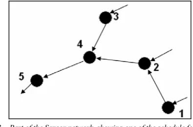
Figure 3. Part of the Sensor network, showing one of the schedule for data transfer

If we consider data aggregation application, GA approach of [3] works fine but if we consider other application where aggregation is not required and instantaneously data to be sent, GA approach will not give desire result. It considers only one time data transfer from node 5 to towards destination and only one time data transfer from node 4 to 5. Hence calculation of energy dissipated will be counted only one time from node 5 to towards destination and node 4 to 5.

But in reality node 4 will send data to node 5 for more than 3 times (one time each for node 1, 2 and 3) and similarly node 5 will send data towards destination for more than 4 times (one time each for node 1, 2, 3 and 4). Here, Energy consumption from node 4 to 5 will be at least 3 times more than the approach of without data aggregation. So, Energy consumption will be more in such case and routing algorithm should consider this scenario.

C. Proposed Fitness Functions for Data Gathering without

Aggregation

For genetic algorithm, encoding scheme, cross over, muta-tion can be derived from the technique discussed in previous chapter. Parent selection method can be selected as roulette wheel, rank based selection or tournament selection method. Termination criteria for genetic algorithm used is N-of-N met-ric [18]. Fitness function used in [3] is for data gathering with aggregation and what we are proposing is for data gathering without aggregation. So, Fitness function will certainly be changed and is discussed next.

1) Total Energy Consumed

Ataul Bari et. al.[13] have suggested Fitness function as discussed earlier in equation 1. This was used for application of data gathering with aggregation. This cannot be used for appli-cation of data gathering without aggregation. We propose total energy consumed by the chromosome (an individual solution in GA) as a fitness function. This total energy can be calculated iteratively. For example, in Fig. 2 (a), base station is node 7 and each node will send data to node 7. This communication can be direct or via some intermediate nodes. Using this new ap-proach, for the solution given in chromosome format, Fig. 2(b), energy consumed can be calculated as summation of the fol-lowing:

• Energy dissipated from node 1 to 3 and node 3 to 7

• Energy dissipated from node 2 to 4 and node 4 to 7

• Energy dissipated from node 3 to 7

• Energy dissipated from node 4 to 7

• Energy dissipated from node 5 to 3 and node 3 to 7

• Energy dissipated from node 6 to 7

2) Minimum Energy Level Concept

Only considering total amount of energy consumed, will not be efficient because it will drain some of the nodes which are on the efficient path. Those nodes will participate in more number of schedules and will get out of energy earlier. This

may result in network partition. This scenario can be avoided and all nodes of the network can take balanced load in terms of energy. This can be achieved by introducing different levels of energy of node. Say, a node having Einit initial energy has an-other mark of energy, Level1 of energy (say 40% of Einit). While making decision for routing, in a path if a node is below Level1 of residual energy, then alternate path is selected with node having more energy than Level1. Out of many possible solutions, those will be strong candidates to win who have more number of nodes having energy greater than Level1. Thus, healthy nodes will participate in routing and weak nodes will get rest, thus overall network lifetime can be extended.

3) Fitness

Fitness will be carrying two parameters, i) total energy con-sumed for the solution (considering without aggregation) and ii) number of nodes below Level1. On the basis of these two parameters, fitness of any solution will be compared.

4) Selecting Best Solution

Out of many solutions, the best solution will be the one, having best fitness value. The solution is considered to be the best solution (having best fitness value) having consuming minimum of energy for that schedule and have minimum num-ber of nodes having residual energy below Level1. If a routing path (a solution) contains minimum energy but having more number of nodes below Level1 of energy, then that solution is over looked and other solution is sought, which is, having min-imum energy consumption and minmin-imum number of nodes below Level1. Thus, solution will contain maximum number of nodes having enough strength and at the same time,

compara-tively less energy consumption.

5) Experimental Results

For our experiments, we have used following first order ra-dio model for communication energy dissipation [19].

m j i t t j i t

T b d b bd E_i( _i, _, )=α_{2 i}+β _{i ,}

Where di,j is the Euclidian distance between node i and j, α2 is the transmit energy coefficient, β is the amplifier coefficient, bti is amount of data to transmit from node i to another node and m is the path loss exponent, 2≤m ≤4. ETi is total transmit energy dissipated.

Similarly, the receive energy, ERi is calculated as follows:

i i

i r r

R b b

E ( )=α1

Where bri is the number of bits received by relay node i and α1 is the receive energy coefficient.

Hence total energy dissipated by a node i for data to receive and then to transmit it further is Ei.

Ei=ETi+ERi

We consider both type of energy in computation of energy consumption. For simulation, the values for the constants are taken same as in [3, 4] as follows:

(i) α1= α2=50 nJ/bit (ii) β=100 pJ/bit/m2 _and

(iii) the path loss exponent, m=4

(iv)The initial energy of each node, Einit=5J.

D. Fitness Functions for Data Gathering with Aggregation

For applications where data gathering requires aggregation, using same approach as discussed above, genetic algorithm approach can be used. Only change requires is in fitness func-tion.

Fitness function will again carry two parameters, i) total en-ergy consumed and ii) number of nodes having residual enen-ergy below Level1. Total energy consumed will not be calculated as discussed in case of without aggregation. Consider the same example of Fig. 3. Now, energy consumption will be calculated for only one time communication between node 4 to node 5 rather than each time to transfer data from node 3 to node 5, node 2 to node 5 and node 1 to node 5. Here we are assuming that data is aggregated at node 4 and all together it is transmit-ted to node 5.

(a)

(b)

(c)

Figure 4. Number of rounds (n/w lifetime) Vs Level1 of energy

We have simulated different networks (with different num-bers of relay nodes) for Warshall’s shortest path first algorithm and then simulated same network with the proposed algorithm. We have also simulated these networks using genetic approach proposed in [3].

Warshall’s algorithm [4 , 5] (sometimes known as the Roy– Floyd algorithm) is a graph analysis algorithm for finding shortest paths in a weighted graph. A single execution of the algorithm will find the lengths (summed weights) of the short-est paths between all pairs of vertices.

Fig. 5 shows comparison between our proposed GA ap-proach with Warshall’s shortest path algorithm. It can be seen

that as the number of nodes in network increases, the perform-ance gets better for GA based approach.

Fig. 6 shows comparison of simulated results for different algorithms for data gathering with aggregation. The GA based approach, proposed GA based approach and Warshall’s short-est path algorithm is compared in the figure.

It can been seen that for smaller size of network, the net-work lifetime (in number of rounds) does not vary much for different methods, but as we increase network size (in terms of number of relay nodes), we can see that GA based approaches can extend life of network for more than 50%. For larger size of network, proposed GA approach gives 7% to 22% extended life of entire network, than that of GA based approach.

Figure 5. Comparison of Warshall’s shortest path and proposed GA approach for data gathering with aggregation.

Figure 6. Comparison of various algorithms for different network size

V. CONCLUSTION

VI. REFERENCES

[1] I.F. Akyildiz, W. Su, Y. Sankarasubramaniam, E. Cayirci, “Wireless sensor networks: a survey”, Computer Networks 38 (4) (2002).

[2] K. Akkaya, M. Younis, “A survey on routing protocols for wireless sensor networks”, IEEE Transactions on Mobile Computing 3 (3) (2005) 325–349.

[3] Ataul Bari, Shamsul Wazed, Arunita Jaekel, Subir Bandyopadhyay “A genetic algorithm based approach for energy efficient routing in two-tiered sensor networks”, Ad Hoc Networks ,Volume 7 , Issue 4, Pages 665-676, ISSN:1570-8705, June 2009

[4] “An explanation on Network flows and Graphs”, [online]. Available: http://www.ieor.berkeley.edu/~ieor266/Lecture12.pdf [Accessed : April 24, 2010].

[5] “A ‘layman’s’ explanation on Floyd–Warshall algorithm”,

[online]. Available : http://en.wikipedia.org/wiki/Floyd%E2%80%93Warshall_algori

thm [Accessed : April 24, 2010].

[6] G. Niezen, “Realization of a self-organizing wireless sensor network,” Final year project report, Pretoria: Department of Electrical, Electronic and Computer Engineering, University of Pretoria, 2005.

[7] Ataul Bari , Arunita Jaekel , Subir Bandyopadhyay, “Clustering strategies for improving the lifetime of two-tiered sensor networks”, Computer Communications, v.31 n.14, p.3451-3459, September, 2008

[8] L. Doherty, B.A. Warneke, B.E. Boser, K.S.J. Pister, “Energy and Performance Considerations for Smart Dust,” International Journal of Parallel Distributed Systems and Networks, 4(3), pp. 121-133, 2001.

[9] G. Anastasi, M. Conti, M. Di Francesco, A. Passarella, “How to prolong the lifetime of wireless sensor networks”, in: M. Denko, L. Yang (Eds.), Mobile Ad hoc and Pervasive Communications, American Scientific Publishers, in press (Chapter 6). http://info.iet.unipi.it/~anastasi/papers/Yang.pdf.

[10] A. Bari, A. Jaekel, S. Bandyopadhyay, “Maximizing the lifetime of two tiered sensor networks”, in: the Proceeding of IEEE

International Electro/Information Technology Conference (EIT 2006), MI, May 2006, pp. 222–226.

[11] D.E. Goldberg, “Genetic Algorithms in Search, Optimization, and Machine Learning”, Addison Wesley, Reading, MA, 1989. [12] Ming-Tsung Chen, Shian-Shyong Tseng, “A genetic algorithm

for multicast routing under delay constraint in WDM network with different light splitting”, Journal of Information Science and Engineering 21 (2005) 85–108.

[13] D.M. Blough, P. Santi, “Investigating upper bounds on network lifetime extension for cell-based energy conservation techniques in stationary ad hoc networks”, in: Proceedings of the 8th ACM International Conference on Mobile Computing and Networking (ACM MobiCom 2002), September 2002, pp. 183–192.

[14] R. Madan, S. Cui, S. Lall, A. Goldsmith, “Cross-layer design for lifetime maximization in interference-limited wireless sensor networks”, in: Proceedings of 24th IEEE Conference on Computer Communications (IEEE INFOCOM 2005), vol. 3, 2005, pp. 1964–1975.

[15] J. Pan, Y.T. Hou, L. Cai, Y. Shi, S.X. Shen, “Topology control for wireless sensor networks”, in: Proceedings of the Ninth Annual International Conference on Mobile Computing and Networking, 2003, pp. 286– 299.

[16] D.E. Goldberg, “Genetic Algorithms in Search, Optimization, and Machine Learning”, Addison Wesley, Reading, MA, 1989. [17] K. Kalpakis, K. Dasgupta, P. Namjoshi, Maximum lifetime data

gathering and aggregation in wireless sensor networks, in: Proceedings of the IEEE International Conference on Networking, 2002

[18] J. Pan, Y.T. Hou, L. Cai, Y. Shi, S.X. Shen, “Topology control for wireless sensor networks”, in: Proceedings of the Ninth Annual International Conference on Mobile Computing and Networking, 2003, pp. 286– 299.