Particle track plotting in Visual MCNP6
Randy Schwarz1,*
1Visual Editor Consultants, PO Box 1308, Richland, WA 99352, USA
Abstract. A visual interface for MCNP6 has been created to allow the plotting of source points, collision points and particle tracks. The interface will allow users to visualize source and collision points based on parameters set by the user. This can be very valuable in understanding the physics of a problem and the important paths that contribute to a tally.
1 Introduction
The Visual Editor is a graphical user interface created for displaying geometry plots and results obtained from the MCNP computer code developed at Los Alamos National Laboratory. It consists of a graphical user interface written in C++ that is linked directly to the MCNP Fortran code.
The Initial creation of the graphical interface started in 1992 and it was first published in 1993 [1]. The original version of the graphical interface was created for Unix/Linux operating systems and was linked to the MCNP computer code [2]. The graphical interface was adapted to the Windows operating system in 1999 [3]. In 2008 the graphical interface was adapted to work with the MCNPX computer code [4].
In 2014 work began on creating a visual Interface for MCNP6 [5]. An initial release of this interface was created to plot geometries and tallies, including mesh tallies and weight window meshes [6]. This paper discusses the latest upgrade of the Visual Editor interface to add source generation point plotting and collision plotting with the option to add particle tracks.
Complete details on these capabilities along and their current status can be found at the Visual Editor website (www.mcnpvised.com).
2 Source point plotting
Sources in MCNP6 can be very complex and it is important to verify that the source geometry is correctly defined. MCNP6 will run even if the source geometry is not correct. Visual tools are required to verify that the source is correct.
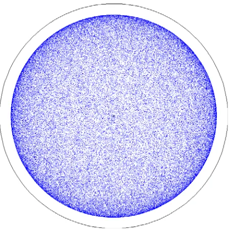
The Visual Editor program is linked to the source generation routine in MCNP6 to obtain the source information so it can be plotted in the Visual Editor. Figure 1 shows a plot in the Visual Editor of a source defined by "SDEF rad=90" inside a sphere of 100 cm. This is a plot of the first 100,000 source points.
Figure 1. Source point plot for sdef rad=90
The user can set a number of parameters for plotting the source points including color and size and how much of the source to plot. Notice in Figure 1, the outside of the sphere is darker than the inside, this is because the source is a shell source and not a spherical volume source. This can be verified, by only plotting particles that are with 10 cm of the plot plane.
Figure 2. Distance from the plot plane set to +/- 10 cm.
It is a common mistake to incorrectly define a spherical volume source as a shell source. The Visual Editor clearly shows this source is a shell source.
Figure 3 shows a how a volume source should look. The source particles should be distributed normally when the distance from the plot plane is set to +/- 10 cm.
Figure 3. Spherical volume source defined correctly.
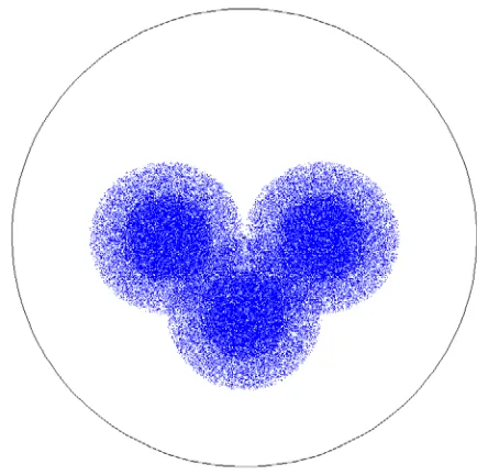
For complex source configurations it is essential that you have a visual confirmation that the source sampling is correct. Figure 4 shows a plot of the source for 3 spheres, 2 have a radius of 50 cm and one has a radius of 30 cm. The source is defined incorrectly because it does not use functional dependence so the two radii are used in all 3 positions. By plotting 100,000 source points the error becomes obvious.
Figure 4. Spherical volume sources without functional dependence.
Without the Visual Editor, users typically look at the first 50 source particles to determine the validity of the source. Figure 5 shows the same source with only 50 source points plotted. From these points it is very hard to determine that the source is wrong.
Figure 5. First 50 particles plotted for wrong source definition.
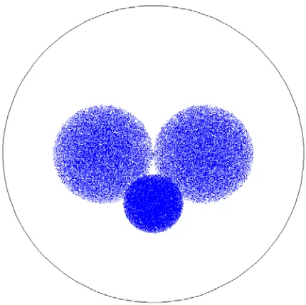
Figure 6. Three Spherical volume sources with functional dependence.
3 Collision point plotting
Because the Visual Editor has access to all of the particle information in MCNP6 it is also possible to plot particle collision points and optionally particle tracks.
Figure 7 shows a plot of collisions displayed from test input file 109 provided with the MCNP6
distribution. This input file has the "tropt" keyword and can only be run in MCNP6. Figure 7 shows the collisions from the first 5 source particles.
Figure 7. Collisions plotted for test input 109
Test input 109 has a proton source hitting a water cylinder producing secondary particles. The mode card has 29 different particle types as shown below
mode n q h g / * z | ! k ? % ^ l b + _ - ~ x c y w o @ u < v >
The color and size of each particle can be set inside the Visual Editor. Figure 8 shows the particle track plotting panel in the Visual Editor for this problem.
Figure 8. particle types listed in the Visual Editor for input 109.
In Figure 8 all particles have the same plot parameters making it difficult to differentiate the different particles plotted in Figure 7.
In Figure 9, we have set the size of the source protons to be larger (using the size column in Figure 8), to differentiate the source protons from the secondary particles created from the source protons.
The color of the particle represents the energy, with the source energy red and the color dropping down to blue for the lowest energy. The Visual Editor tabulates the energy of all particles that it displays and sets this energy range dynamically. The user can set a specific energy range by specifying a minimum and maximum value in the table shown in Figure 8.
To determine the secondary particles being generated, we now turn off the plotting of the source protons by unselecting the "Show" column in Figure 8. We then set the size and color of the secondary particles to differentiate them as shown in the particle track plotting panel in Figure 10.
Figure 10. Secondary particles differentiated by color.
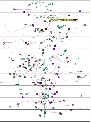
Figure 11 now shows the collisions colored by particle type for the first 5 particles.
Figure 11. Secondary particles differentiated by size and color.
By comparing the table in Figure 10 with the plot in Figure 11, it is possible to now differentiate some of the secondary particles. The yellow particle moving to the right in the top center is a muon (particle type |). The small green dots are neutrons, The large purple dots are muon neutrinos (particle type v). The orange dots are electron neutrinos (particle type u).
The user may spend a significant amount of time setting particle size and color, so the option is provided to save this information for this input file by selecting the "Save Parameters" option in the menu shown in Figure 10.
To determine the path of the particles that cause the collisions, it is possible to turn on tracks as shown in Figure 12. Here tracks have been turned on for neutrons by selecting the tracks column in Figure 10. The color of the tracks has been set to magenta and the size has been slightly increased over the default size so that they show up better.
Figure 12. Particle tracks plotted for neutrons
4 Plotting collision points showing
variance reduction
The ability to visually differentiate different particle types within the plot is critical for understanding the physics of the problem. However, just as important is the ability to plot particle tracks from variance reduction.
Figure 13. Source points plotted for a transportation cask showing source biasing.
Figure 14 shows the axial source biasing of the 16 pins. The source points are colored by weight. The under-biased source points at the bottom are red and the over-biased source particles at the top are blue.
Figure 14. Source points plotted for a transportation cask showing axial source biasing.
Figure 14 shows both the presence of the radial biasing and the axial biasing. The distance from the plot plane has been set to 4 cm so the source points in the other pins do not show up in the plot.
Figure 15 shows an axial plot of collision points in the transportation cask shown previously in figures 13 and 14. The particles are being directed toward the tally volume outside the cask using variance reduction. The collision points are colored by weight, with the source particles being red and the low weight particles colored
in blue. The effects of the variance reduction can be clearly seen.
Figure 15. Collision points showing variance reduction.
The collisions can be plotted on top of any normal MCNP6 geometry plot, including color plots. Figure 16 shows the collision points plotted on top of a color plot of the importances. Since the collisions occur due to the presence of the importances, it can be very useful to verify the importance mapping along with the collision points.
Figure 16. Collision points plotted with importance colors.
Figure 17 shows a plot similar to that in Figure 16, expect now only those particles that contribute to the tally are plotted. Since only a few tracks will contribute, it is necessary to plot a lot more tracks to see the important tracks for the tally.
Figure 17. Collision that contribute to the tally.
Figure 18 shows a close up view of only those collisions that reach the tally volume. The track option has been turned on to show the path of the particles. The size and color of the track lines can be set by the user.
Figure 18. Particle tracks that contribute to the tally.
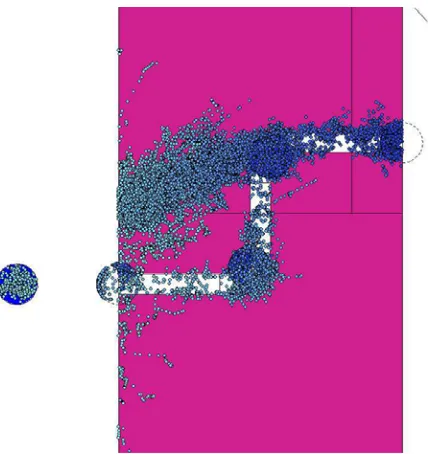
Particle tracks can also be shown for DXTRAN spheres. Figure 19 shows a shielding problem that consists of a hole in a concrete wall with a 1 MeV neutron source inside a sphere.
Figure 19. Tracks showing contributions to DXTRAN spheres.
This problem also includes weight windows since part of the contribution to the final tally is from particles moving through the concrete shield. In Figure 20, we plot the collisions on top of the weight window color mesh.
Figure 20. Collisions plotted on top of the weight windows mesh.
Figure 21. Tracks plotted on top of weight windows.
Sometimes it may be desirable to plot the collisions on top of a mesh tally. In Figure 22, we plot the collisions on top of a fmesh tally.
Figure 22. Collisions plotted on top of an fmesh tally.
5 Criticality source point plotting
For criticality calculations (KCODE source) it is essential to verify that all fissionable regions have been adequately sampled. There are calculational methods that can be used to help verify if the source is properly sampled, but they do not always work for complex critical systems.
The Visual Editor has the ability to plot the cycle-by-cycle source points for a criticality calculation so that the user can verify that the source has converged properly and that all points of interest have been sampled.
Figure 23 shows all the fission points sampled for a criticality calculation for a sub-critical system.
Figure 23. Fission points sampled for a KCODE calculation.
The fission points can be sampled for each cycle and an animation can be made of the points from cycle to cycle. Figure 24 shows the fission source distribution for the first cycle. The calculation was initiated with a single point at the center of the lattice which can be clearly seen in this plot.
Figure 24. Fission points for the first cycle.
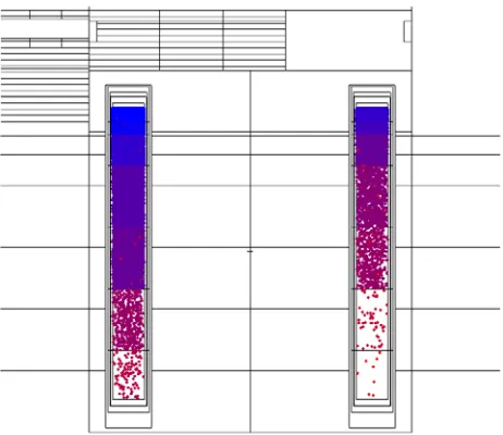
Figure 25. Fission source points plotted for a non-converged criticality calculation.
This plot clearly shows that the most important fission volume at the top has not been sampled. Without the ability to visualize the location of the fission source points it is very hard to verify that the value of Keff is correct. The value calculated for this source location is 0.58, while the true value of Keff for the geometry which is dominated by the upper volume is 1.01.
The ability to plot the source point locations for a criticality calculation can provide valuable insight into the propagation of the fission points as a function of cycle.
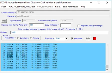
Figure 26 shows the panel used for plotting the fission points. The user has a number of options including which cycles to plot and the size and color of the points to plot. For animations, the user can select the delay time (in milliseconds) between the different cycles.
Figure 26. Panel for displaying criticality fission points.
To correctly sample the entire volume we use a cylindrical source to sample points up and down the central cylinder for the first cycle. Figure 27 shows the
plot of the fission points for this calculation which will now calculate the correct value of Keff.
Figure 27. Fission source points, showing a converged source sampling.
4 Conclusion
The Visual Editor is a graphical user interface for MCNP6. The ability to plot the source and collisions allow the user to user to gain valuable insight into the source configuration and particle behavior. This is done in a user friendly easy to use interface.
References
1. R.A. Schwarz, L.L. Carter, T.P. Dole, S.M. Fredrickson, and B.M. Templeton,
Trans. Am.
Nucl. Soc
.,
69, 401 (1993)2. J. F. Briesmeister, Ed., ``MCNP--A General Monte Carlo Code for Neutron and Photon Transport, Version 3A,'' Los Alamos National Laboratory report LA-7396-M, Rev. 2 (1986)
3. L.L. Carter, R.A. Schwarz, and J. Pfohl, Trans. Am. Nucl. Soc., 81, 256–257 (1999).
4. L.L. Carter, R.A. Schwarz, and A. L. Schwarz, NASA contract number NNL07AA10C (2008) 5. D. B. Pelowitz, Ed., ``MCNP6 Users Manual
Version 1.0,'' Los Alamos National Laboratory report LA-CP-13-00634 (2013).