Deep Learning using Restricted Boltzmann
M
achines
Neelam Agarwalla1, Debashis Panda2, Prof. Mahendra Kumar Modi3
1,2,3
Distributed Information Centre, Department of Agricultural Biotechnology, Assam Agricultural University, Jorhat-785013, India
3
Professor/HeadDepartment of Agricultural Biotechnology, Assam Agricultural University, Jorhat 785013, Assam, India
Abstract :- Restricted Boltzmann machines (RBM) are probabilistic graphical models which are represented as stochastic neural networks. Increase in computational capacity and development of faster learning algorithms, led RBMs to become more useful for many machine learning problems. RBMs are the building blocks of many deep multi-layer architectures like Deep Belief networks (DBN) and Deep Boltzmann Machines (DBM). Many machine learning algorithms like neural networks with a few hidden layers, Support Vector Machines (SVM), k-Nearest Neighbors (k-NN), etc., are shallow architectures but DBNs and DBMs are deep architectures with many hidden layers. In this paper we have compared two different inference models with four different architectures. Experimental comparisons demonstrate that both the inference vary according to the number of hidden layers and number of neurons in it.
Keywords - RBM, DBN, DBM, SVM, k-NN, DNN
I. INTRODUCTION
Many existing machine learning algorithms exhibit “shallow” architectures. For example, neural networks with a few hidden layers, kernel regression, k-Nearest Neighbors, Support Vector Machines, and many others have shallow architectures. But some functions cannot be efficiently represented by architectures that are too shallow because they are incapable of efficiently extracting some types of complex structure from rich sensory input. Moreover, training these systems requires large amount of labeled data. Thus it would be worthwhile to explore learning algorithms for deep architectures, which might be able to represent some functions otherwise not efficiently representable. One characteristic of deep architecture is that it can make efficient use of unlabeled data. But training deep generative models is a difficult task, because performing inference and evaluating marginal probabilities under such models is complicated. The revolution to effective training strategies for deep architectures came in 2006 with the introduction of algorithms for training Deep Belief Networks (DBN) [8] and stacked auto-encoders [7], which are all based on a similar approach of greedy layer-wise unsupervised pre-training followed by supervised fine-tuning.
Some of the areas where deep learning architectures have been successfully applied are classification tasks [6], regression [9], dimensionality reduction [7], information retrieval and natural language processing [10].
In a previous paper [16], the working of restricted Boltzmann Machine has been briefly explained. Different techniques have been proposed to improve generalization ability. A dropout training is a technique to improve the generalization ability by dropping several hidden nodes during the training process [12]. But it is computationally intensive. So, fast algorithm of the dropout training has been reported[13]. The main component of the DNN training is a restricted Boltzmann Machine (RBM). It is initialized by stacking RBM.
II. RESTRICTED BOLTZMANN MACHINE (RBM)
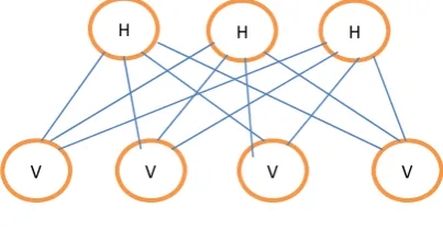
Boltzmann Machines (BM) is the form of log-linear Markov Random Field (MRF), where the energy function is linear in its free parameters [4]. We can introduce hidden nodes to make them powerful enough to represent complicated distribution. By introducing more hidden variables, we can increase the modeling capacity of the Boltzmann Machine. Restricted Boltzmann Machines are BMs without visible-visible and hidden-hidden connections [4]; hence the name ‘restricted’. A graphical representation of an RBM is shown below.
Fig. 1 A graphical representation of an RBM
The Energy function E (v, h) is given by:
E(v,h)= – b’v – c’h – h’Wv (1)
where W represents the weights connecting hidden and visible units and b, c are the offsets of the visible and hidden layers respectively.
In context to free energy, eq (1) is given by:
F (v) = – b’v – ∑i log ∑hi e hi (ci+Wiv)
H H H
RBMs are conditionally independent given one another so they can be written as:
p (h | v) = ∏ |
p (v | h) = ∏
RBMs with binary unit where vj and hi Є {0, 1}
can be obtained by:
p(hi=1|v)=sigm(ci+Wiv) (2)
p(vj=1|h) = sigm(bj+W’jh) (3)
Now, the free energy is given by:
F(v) = – b’v– ∑ilog(1+e(ci+Wiv)) (4)
Combining (1) and (4), we get log-likelihood gradients of RBM as follows:
= Ev[ | . vj ]– vj(i). sigm(Wi . v(i) +cj)
= Ev[ | ] – sigm ( Wi . v(i) )
= Ev[ ]–vj(i) (5)
Sampling of RBM can be done by running a Markov chain to convergence, using Gibbs sampling as the transition operator.
A. Gibbs Sampling
Gibbs sampling of N random variables S = (S1 ,…,
SN) is done through a sequence of N sampling sub-steps of
the form Si ~ p(Si| S-i) where S-I contains theN-1 other
variables in S excluding Si [4].
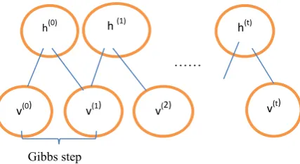
In RBMs the set of visible and hidden units are conditionally independent, so we can perform block Gibbs sampling by simultaneously sampling visible units, given fixed values of hidden units. Similarly hidden units can also be sampled, given visible units. One step of Markov chain is given by:
h(n+1) = sigm ( W
’v(n) +c)
v(n+1) = sigm ( Wh(n+1) +b)
where hn is the set of all hidden units at the n-th
step of the Markov chain
Fig. 2 Graphical representation of Gibbs Sampling
The accurate samples of p(v, h) is given by samples(v(t) , h(t)) when t
→ ∞
Here updation of each parameter in the learning process would require running one such chain to convergence, which is computationally intensive. This is fundamentally why the Boltzmann machine was replaced in the late 80’s by the back-propagation algorithm for multi-layer neural networks as the dominant learning approach. However, recent works [11], [1], [2] have shown that short chains can sometimes be used successfully, and this is the principle of Contrastive Divergence (CD), discussed below to train RBMs.
B. Contrastive Divergence
CD uses two tricks to speed up the sampling process [4], [11]:
• CD does not wait for the chain to converge.
Samples are obtained after only k-steps of Gibbs sampling.
• It initializes the Markov chain with a training
example so that the chain will already be close to p having converged to its final distribution p. It has been shown that estimates obtained after running the chain for just a few steps can be sufficient for model training [11]. The single-step contrastive divergence algorithm (CD-1) works like this:
Positive phase
• An input sample v is clamped to the input layer. • v is propagated to the hidden layer
• Hidden layer activation result is h
Negative phase
• Propagate h back to the visible layer with result v’
• Propagate the new v’ back to the hidden layer with activations result h’ Weight update
w(t +1) = w(t) + a(vhT + v
’h’T ) (6) where ‘a’ is the learning rate and v, v’, h, h’, and w are vectors.
III. MODELS OF DEEP ARCHITECTURE A. Introduction
Learning algorithms that learn to represent functions with many levels of composition are said to have a deep architecture. Deep architectures are composed of multiple levels of non-linear operations, such as in neural nets with many hidden layers. RBMs are the building blocks of deep architectures such as DBN and DBM. Some of the deep learning models are:
B. Deep Belief Network (DBN)
The first model is the Deep Belief Net (DBN) by Hinton [1], obtained by training and stacking several layers of Restricted Boltzmann Machines (RBM) in a greedy manner. Once this stack of RBMs is trained, it can be used to initialize a multi-layer neural network for classification [5].
A DBN is a multi-layer generative model with layer variables h0 (the input or visible layer), h1, h2, etc. The
top two layers have a joint distribution which is an RBM, where P(hk|hk−1) is parametrized in the same way as for an RBM. Hence a 2-layer DBN is an RBM, and a stack of RBMs share parametrization with a corresponding DBN.
h(0) h (1) h(t)
v(0) v(1) v(2) v(t)
Gibbs step
The contrastive divergence update direction can be used to initialize each layer of a DBN as an RBM, as follows. Consider the first layer of the DBN trained as an RBM P1
with hidden layer h1 and visible layer v1. We can train a
second RBM P2 that models (in its visible layer) the
samples h2 from P1(h1|v1) when v1 is sampled from the
training data set. It has been shown in [6] that this maximizes a lower bound on the log-likelihood of the DBN. The number of layers can be increased greedily, with the newly added top layer trained as an RBM to model the samples produced by chaining the posteriors P(hk|hk−1) of the lower layers (starting from h0 from the training data set)
[6].
1) Greedy layer wise training
It first trains the lower layer with an unsupervised learning algorithm (such as one for the RBM), giving rise to an initial set of parameter values for the first layer of a neural network. Then use the output of the first layer (a new representation for the raw input) as input for another layer, and similarly initialize that layer with an unsupervised learning algorithm. After having thus initialized a number of layers, the whole neural network can be fine-tuned with respect to a supervised training criterion as usual [5].
2) Advantages
First, the greedy layer-by layer learning algorithm can find a good set of model parameters fairly quickly, even for models that contain many layers of nonlinearities and millions of parameters. Second, the learning algorithm can make efficient use of very large sets of unlabeled data, and so the model can be pre-trained in a completely unsupervised fashion. Finally, there is an efficient way of performing approximate inference to compute the values of the latent variables in the deepest layer, given some input [2].
3) Disadvantages
A critical disadvantage of this greedy algorithm is that the approximate inference procedure is limited to a single bottom-up pass. One consequence of ignoring top-down influences on the inference process is that the model can fail to adequately account for uncertainty when interpreting ambiguous sensory inputs. Moreover, the existing greedy procedure is clearly suboptimal: it learns one layer of features at a time and never re-adjusts its lower-level parameters. Although global fine-tuning using the contrastive wake-sleep algorithm has been used by Hinton, it is very slow and inefficient [2].
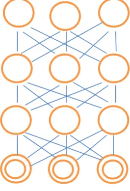
Fig. 3 Graphical Representation of Deep Belief Network
C. Deep Boltzmann Machine (DBM)
A Deep Boltzmann Machine is a network of symmetrically coupled stochastic binary units. It contains a set of visible units v ∈ {0, 1}, and a sequence of layers of hidden units h1 ∈ {0, 1}F1 , h2 ∈ {0, 1}F2 ,..., hL ∈ {0, 1}FL.
There are connections only between hidden units in adjacent layers, as well as between the visible units and the hidden units in the first hidden layer[3].
1) Advantages
First, it retains much of the requisites found in Deep Belief Networks: it discovers several layers of increasingly complex representations of the input, it comes with an efficient layer-by-layer pre-training procedure, it can be trained on unlabeled data and can be fine-tuned for a specific task using the (possibly limited)labeled data. Second, the approximate inference procedure for DBM’s incorporates a top-down feedback in addition to the usual bottom-up pass, allowing Deep Boltzmann Machines to better incorporate uncertainty about ambiguous inputs. Third, the parameters of all layers can be optimized jointly by following the approximate gradient of a variational lower-bound on the likelihood function. This greatly facilitates learning better generative models.
2 ) Disadvantages
The approximate inference, which is based on the mean-field approach, is considerably (between 25 and 50 times) slower compared to a single bottom-up pass as in Deep Belief Networks. This makes the joint optimization of DBM parameters impractical for large datasets. It also reduces the appeal of using DBM’s for extracting useful feature representations, since the expensive mean-field inference must be performed for every new test input.
Fig. 4 Graphical Representation of DBM
IV. DIFFERENT INFERENCES OF THE RBM
the random variables which means that the calculation with the probabilities takes the expectation after applying the activation function [15].
A. Inference of the Conventional Algorithm
A deep belief network is formed by stacking the trained RBMs. First, the RBM is pre-trained with training data by the CD training algorithm. Then, the states of the binary hidden units of the trained RBM are used as the training data of the next layer of the RBM. This process is repeated to many layers [15] .
In the DNN, the output of the (l +1) - th layer’s nodes are calculated by
ql + 1 = σ(WTlql + bl) (7)
Where, ql is the output of the l-th layer’s nodes.
Here the probabilities or the expectation of the random binary variables are used as the output of the nodes.
ql = P(ξl = 1) = Epξl [ξl] (8)
Where, ξl represents the associated random binary variables.
The probabilities of the (l +1) th node’s state are inferred by
P(ξl +1 = 1) = σ(WT
lEpξl[ξl] + bl) (9)
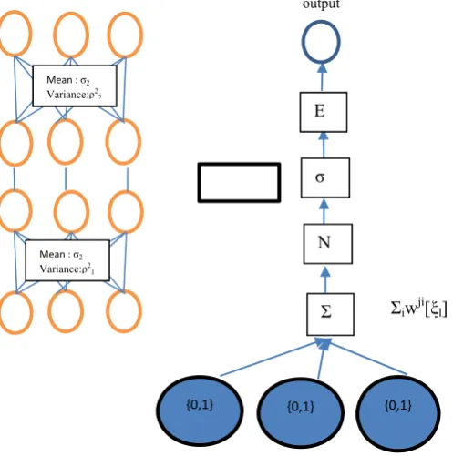
B. New Inference of the RBM
Here, the inference of the RBM taking expectation after the activation function as it is expected to take expectation as late as possible. The new inference is expressed by
P(ξl +1 = 1) = Epξl [σ (WTl [ξl] + bl) (10)
The difference between the two inferences are in the place of taking the expectation. In the new inference, conditional probabilities of the (l+1)th node’s state given every possible combination of the binary states of the l-th node are evaluated. Then the expectation of those evaluated conditional probabilities is evaluated to infer the probabilities of the ( l + 1) th node’s state[14].
output
Input random Binarystates Fig. 5 Conventional Inference
output
Input random Binarystates
Fig. 6 New Inference
1) Fast Dropout Training
In the new algorithm, closed form approximation of the fast drop-out training is used [13][14]. A random variable Sl+1j is associated to the input of the activation of
the j-th node in the l +1-th layer
Sl+1j = wljTξl + blj (11)
Where wlj is the j-th column vector of the matrix Wl
and blj is the j-th element of the vector bl
The density distribution of this random variable is approximated by Guassian distribution
Sl+1j ˜ N(Sl+1j | µ,ρ2) (12)
Where, N(Sl+1j|µ,ρ2) represents the guassian distribution
whose mean is µ and variance is ρ2.
Mean is given by
µ = E [Sl+1j ] = E[wljTξl + blj ]
= Σ wlijp(ξli=1) + blj (13)
Variance is given by
ρ2 = V[Sl+1j ] = V[wljTξl + blj]
= Σ wlij2p(ξli=1){1 – p (ξli=1)} (14)
Where V[x] represents the variance of the variable x, wij is
the (i, j)-th element of the vector (ξli is the i-th element of
the vector ξl[14][15]. Mean : σ2
Mean : σ2
σ
Σ
E E E
ΣwjiE[ξl]
{0,1} {0,1} {0,1}
Mean : σ2
Variance:ρ2 2
Mean : σ2
Variance:ρ2 1
E
σ
N
Σ
{0,1} {0,1} {0,1}
V. EXPERIMENTAL VALIDATION
Here we have evaluated both the inference with the dataset:MNIST. The MNIST handwritten digit dataset consists of 28*28 sized black and white images, each containing a digit 0 to 9 (10 - classes). It includes 60,000 training images and 10,000 test images.
I. Conventional Inference
In this inference we have built five different architectures with different number of hidden layers and also different number of hidden neurons in same architecture. This comparison is demonstrated below in the table:
Table I. Comparison of Conventional Inference
No. of hidden layer
No. of neurons in each hidden layer
Train error
Test
error Misclassfied
2 800, 800 6.346 12.676 117
2 1200, 1200 4.896 11.615 111
3 500,500,2000 6.247 11.513 115
3 500,1000,2000 6.163 11.705 106
4 500,500,1000,2000 3.281 14.034 112
II. New Inference
We have used the same number of hidden layers and hidden neurons in accordance with the conventional inference. Here the RMSE and error rate is calculated as in [14]. The comparison is shown in the table below:
Table II. Comparison of new Inference
No. of hidden layer
No. of neurons in each hidden layer
Training Data Testing Data
RMSE Error
rate RMSE Error
rate 2 800, 800 0.0162 0.002 0.0544 0.017 2 1200, 1200 0.017 0.0022 0.0559 0.0167 3 500,500,2000 0.022 0.0044 0.0612 0.0201 3 500,1000,2000 0.0234 0.0041 0.0623 0.0206
4 500,500,1000,2000 0.0206 0.0034 0.0608 0.0211
VI. CONCLUSION
In deep learning, we learn to predict and interpret complex dependencies between the input (observed) features. In a deep algorithm, the input is passed through several non-linearities before giving the output. Most modern learning algorithms (including decision trees, SVMs and naive bayes) are "shallow".
In this paper, we have found the conventional inference as proposed by Hinton that the misclassification error varies a lot with the number of hidden neurons and number of hidden layers. But increasing the number of hidden layers to four increases the Computational Complexity and it yields unsatisfactory result as compared to three hidden layers. But in new inference as proposed by Tanaka, increasing in the number of hidden layer does yield much effective changes in the result. We need to increase the number of hidden layers. Our future will be to implement both the algorithm in the biological datasets.
ACKNOWLEDGMENT
Authors 1 & 2 were financially supported by Biotechnology Information System Network (BTISNET), Department of Biotechnology, Government of India.
REFERENCES
[1] Yoshua Bengio, “Learning deep architecture for AI”, Foundation and trends in Machine Learning,Volume 2 Issue 1,pages 1-127, January 2009.
[2] Ruslan Salakhutdinov, Hugo Larochelle , “Efficient Learning of Deep Boltzmann Machines ”,Neural computation, ,Volume 24,No.8, Pages 1967-2006, August 2012.
[3] Geoffrey Hinton, Ruslan Salakhutdinov, “Deep Boltzmann machine”, In 12th International Conference on Artificial Intelligence and Statistics (AISTATS), Volume 5 of JMLR, Florida, USA, 2009.
[4] Asja Fischer and Christian Igel, “ An Introduction to Restricted BoltzmanMachine”, Progress in Pattern Recognition , Image analysis, Computer Vision and Applications, Volume 7441,pp 14-36, ISBN : 978-3-642-33274-6 ,2012
[5] D. Erhan, Y. Bengio, A. Courville, P.-A. Manzagol, P. Vincent, and S. Bengio, “Why does unsupervised pre-training help deep learning? ”, Journal of Machine Learning Research, JMLR, 11:625-660, 2010.
[6] Bengio, Y., & LeCun, Y., “Scaling learning algorithms towards AI”, In Bottou, L., Chapelle, O., DeCoste, D., & Weston, J. (Eds.), Large Scale Kernel Machines. MIT Press, 2007.
[7] Salakhutdinov, R., & Hinton, G. E. (2007a), “Learning a nonlinear embedding by preserving class neighbourhood structure”, In Proceedings of the Eleventh International Conference on Artificial Intelligence and Statistics (AISTATS’07) San Juan, Porto Rico. Omnipress, 2007.
[8] Hinton, G. E., “To recognize shapes, first learn to generate images”, Tech. rep. UTML TR 2006-003, University of Toronto, 2006. [9] Salakhutdinov, R., & Hinton, G. E., “Using deep belief nets to learn
covariance kernels for Gaussian processes”, In Platt, J., Koller, D., Singer, Y., & Roweis, S. (Eds.), Advances in Neural Information Processing Systems 20 (NIPS’07), pp. 1249–1256 Cambridge,MA. MIT Press, 2008.
[10] Mnih, A., & Hinton, G. E., “A scalable hierarchical distributed language model”, In Koller, D.,Schuurmans, D., Bengio, Y., & Bottou, L. (Eds.), Advances in Neural Information Processing System 21 (NIPS’08), pp. 1081–1088., 2009.
[11] G. E. Hinton, “Training products of experts by minimizing contrastive divergence”, Neural Computation, 14(8):1771 - 1800,
Aug. 2002.
[12] L. Wan, M. Zeiler, S. Zhang, Y. L. Cun, and R. Fergus, “Regularization of neural networks using dropconnect,” in
International Conference onMachine Learning (ICML), 2013, pp. 1058–1066.
[13] S. Wang and C. Manning, “Fast dropout training,” in International Conference on Machine Learning (ICML), 2013, pp. 118–126. [14] G. Hinton, “A practical guide to training restricted boltzmann
machines,”UTML TR 2010-003, 2010.
[15] M. Tanaka and M. Okutomi, “A Novel Inference of a Restricted Boltzmann Machine,” Proceedings of the 2014 22nd International Conference on Pattern Recognition (ICPR ) 2014, pp. 1526-1531. [16] Adarsh Pradhan and Neelam Agarwalla,”Deep Learning using
Resticted Boltzmann Machine,” in International Journal of Advanced Computer and Engineering, Volume4, Issue3 2015,
pp10-14