Numerical Integration by Different Numerical Techniques

ISSN 2286-4822

www.euacademic.org DRJI Value: 5.9 (B+)

Numerical Integration by Different Numerical

Techniques

ZAINAB HASAN MSHEREE

MSC student, Department of Mathematics and Statistics Foundation of Technical Education Technical Instructors Training Institute, Baghdad Iraq

MOHAMMED MUKHEEF ABED

MSC student, Department of Mathematics and Statistics Foundation of Technical Education Technical Instructors Training Institute, Baghdad Iraq

Abstract:

Key words: Strategic Content Learning, Mathematics, Achievement, Gender and Learning Disability

I. Introduction

cubature, although the meaning of quadrature is understood for higher dimensional integration as well. The basic problem in numerical integration is to compute an approximate solution to a definite integral.



b

a

dx

x

f

(

)

If f(x) is a smooth function integrated over a small number of dimensions, and the domain of integration is bounded, there are many methods for approximating the integral to the desired precision.

Fig (1.1) Numerical integration consists of finding numerical approximations for the value

S

.

Methodology

On the basis of available literature we have studied different methods of numerical integration: Trapezoidal, Simpson’s One-Third and Simpson’s Three-Eight, Gaussian Integration, Euler-McLaren Integration and Romberg Integration. Using these methods we have solved numerical problems, and done a comparative study of these methods. We have also solved nonlinear integration problem of civil engineering by using

numerical integration. Newton-cote’s Quadrature Formula:

Let





b a

ydx

I

where y takes the values

y

₀

,

y

₁

,

y

₂

,...

..,

y

_nfor

n

x

x

x

x

sub-intervals, each of width

n a b

h  so that

.

.,

,...

2

,

,

_{1 0 2 0 0}

0

a

x

x

h

x

x

h

x

x

nh

b

x











_n













x nh

x

f

x

dx

I

0 0

)

(

                ... 24 ) 2 ( 12 ) 3 2 ( 2 0 3 2 0 2 0 0 y n n y n n y n y nh

I (1)

This is a general quadrature formula and is known as

Newton-Cote’s quadrature formula. A number of important deductions viz. Trapezoidal rule, Simpson’s one-third and three-eighth rules, can be immediately deduced by putting n = 1, 2 and 3 respectively, in formula (1).

Trapezoidal Rule (n = 1).

Putting n = 1 in formula (1) and taking the curve through

(

x

₀

,

y

₀

)

and

(

x

₁

,

y

₁

)

as a polynomial of degree one so that differences of order higher than one vanish, we get



























_

_



h x

x

y

y

h

y

y

y

h

y

y

h

dx

x

f

0 0

)

(

2

)]

(

2

[

2

2

1

)

(

_{0 0 0 1 0 0 1}

Similarly, for the next sub-interval

(

x

₀



h

,

x

₀



2

h

)

, we get







        h x h x nh x h n

x yn yn

h dx x f y y h dx x f 2 ) 1 ( 1 2 1 0 0 0 0 ) ( 2 ) ( ...., ),... ( 2 ) (

Adding the above integrals, we get



       

nh x

x y yn y y yn

h dx x f 0 0 )] ... ( 2 ) [( 2 )

( _{0 1 2 1}

This is known as Trapezoidal rule. By increasing the number of

subintervals, thereby making h very small, we can improve the

Simpson’s One-Third Rule (n = 2).

Putting n = 2 in formula (1) and taking the curve through

(

x

₀

,

y

₀

)

,

(

x

₁

,

y

₁

)

and

)

,

(

x

₂

y

₂ as a polynomial of degree two so that differences of order higher than two vanish, we get,



x h



_











_



x

f

x

dx

h

y

y

y

2 0 2 0 0 0 0

6

1

2

)

(

) 4 ( 3 )] 2 ( ) ( 6 6 [ 6 2 2 1 0 0 1 2 0 1

0 y y y

h y y y y y y

h _{       }



Similarly,





   

h x

h

x y y y

h dx x f

4

2 2 3 4

0 0 .., ),... 4 ( 3 ) (



       nh x h n n

x yn yn yn

h dx x f

0

0 ( 2) 2 1

) 4 ( 3 ) (

Adding the above integrals, we get,



            

nh x

x y yn y y yn y y yn

h dx x f 0 0 )] ... ( 2 ) ... ( 4 ) [( 3 )

( _{0 1 3 1 2 4 2}

This is known as Simpson’s one-third rule.

While using this formula, the given interval of integration must be divided into an even number of sub-intervals, since we find the area over two sub-intervals at a time.

Simpson’s Three-Eight Rule (n = 3).

Putting n = 3 in formula (1) and taking the curve through

(

x

₀

,

y

₀

)

,

(

x

₁

,

y

₁

)

,

)

,

(

x

₂

y

₂ and

(

x

₃

,

y

₃

)

as a polynomial of degree three so that differences of order higher than two vanish, we get,

















_

_

_

_

_

_



h x

x

f

x

dx

h

y

y

y

y

3 0 3 0 2 0 0 0 0

8

1

4

3

2

3

3

)

(

)] 3 3 ( ) 2 ( 6 ) ( 12 8 [ 8 3 0 1 2 3 0 1 2 0 1

0 y y y y y y y y y

y h           ] 3 3 [ 8 3 3 2 1

0 y y y

y

h _{  }



Similarly,





    

h x

h

x y y y y

h dx x f

6

3 3 4 5 6



        

h x

h n

x yn yn yn yn

h dx x f 6 ) 3

( 3 2 1

0 0 ] 3 3 [ 8 3 ) (

Adding the above integrals, we get,



                

nh x

x y yn y y y y yn yn y y yn

h dx x f 0 0 )] ... ( 2 ... ( 3 ) [( 8 3 )

( _{0 1 2 4 5 2 1 3 6 3}

This is known as Simpson’s three-eighth rule.

While using this formula, the given interval of integration must be divided into sub-intervals whose number n is a multiple of 3.

Errors in Quadrature Formula:

If

y

_p is a polynomial representing the function y f(x) in the interval [a,b]

then error in the quadrature formulae is given by









b

a

b a

y

p

dx

dx

x

f

E

(

)

(2)

Error in Trapezoidal Rule:

Expanding y f(x)in the neighborhood of

x



x

₀ by Taylor’s series, we get

...

!

2

)

(

)

(

"₀

2 0 ' 0 0 0













y

x

x

y

x

x

y

y

(3)





             x h

x y dx

x x y x x y ydx 0 0 ... ! 2 ) ( )

( 0"

2 0 ' 0 0 0

...

!

3

!

2

'' ' 0 3 " 0 2

0









hy

h

y

h

y

(4)

Now, area of the first trapezium in the interval ( )

2 ]

,

[x₀ x₁  A₁  h y₀ y₁ (5)

Putting

x



x

₀



h

,

y



y

₁ in (4.3),

...

!

2

" 0 2 ' 0 0

1







y



h

hy

y

y

(6)

From (5) and (6), we get

.... ! 22 ! 2 ... ! 2 2 " 0 3 ' 0 2 0 " 0 2 ' 0 0 0

1    

        

 h y y hy h y hy h y h y

Subtracting eqn. (7) from eqn. (4) gives the error in

(

x

₀

,

x

₁

),



_           '' 0 3 " 0 3 1 12 ... ! 2 2 1 ! 3 1 y h y h A

ydx Neglecting other terms

Similarly, the error in

[

x

₁

,

x

₂

]

is ₁"

2

12

y

h



and in

[

x

_n1

,

x

_n

]

is " ₁

3

12





n

y

h

.

Hence the total error is

)

...

(

12

'' 1 '' 1 '' 0 3 











h

y

y

y

_n

E

Let y"(),ab be the maximum of

|

y

₀"

|,

|

y

₁"

|,...

,

|

y

"_n1

|

then, we have

)

(

"

12

)

(

)

(

"

12

2 3





b

a

h

y

y

nh

E











nh

a

b





Hence the error in the trapezoidal rule is of order h2_.

Error in Simpson’s 1/3rd _Rule:

Integrating eqn. (4.3) with respect tox between the limits x0 and x2.





             2 0 0 0 2 _" 0 2 0 ' 0 0 0 ... ! 2 ) ( ) ( x x h x

x y dx

x x y x x y ydx

...

!

5

32

!

4

16

!

3

8

2

2

₀( )

5 " 0 4 " 0 3 ' 0 2

0













iv

y

h

y

h

y

h

y

h

hy

(8)

Now, ( 4 )

3 0 1 2

1 y y y

h

A    (9)

Where A1 is the area of the curve in the interval

[

x

₀

,

x

₂

]

.

Putting

x



x

₀



h

,

y



y

₁ in (2), we get

...

!

3

!

2

'' ' 0 3 '' 0 2 ' 0 0

1









y



h

y

h

hy

y

Putting

x



x

₀



2

h

,

y



y

₂ in (2), we get

...

!

3

8

!

2

4

2

₀'''

3 '' 0 2 ' 0 0

2









y



h

y

h

hy

y

y

(11)

Substituting eqns. (10) and (11) in eqn. (4.9), we get

....

18

5

3

2

3

4

2

2

₀( )

5 '' ' 0 4 '' 0 3 ' 0 2 0

1













iv

y

h

y

h

y

h

y

h

hy

A

(12)

Now, the error in interval

[

x

₀

,

x

₂

]

is given by















 





2 0

....

18

5

15

4

( )

0 5 1 x x iv

y

h

A

ydx

) ( 0 5

90

iv

y

h





Neglecting terms of order

h

6

,

h

7

,...

Similarly, the principal part of error in interval [x2,x4] is

) ( 2 5

90

iv

y

h





and so on.

Hence total principal error is

]

....

[

90

) ( ) 1 ( 2 ) ( 2 ) ( 0 5 iv n iv iv

y

y

y

h

E











_

Let

y

(iv)

(



)

be the maximum of

|

y

₀(iv)

|,

|

y

₂(iv)

|,...,

|

y

₂(iv_n)₁

|

Then, we have,

(

)

180

)

(

)

(

90

) ( 4 ) ( 5





iv iv

y

h

a

b

y

h

E











Hence, the error in the Simpson’s (1/3)rd rule is or order h4_.

Similarly, the principal part of the error for Simpson’s (3/8)th rule is ( )

5

80

3

_iv

y

h



in the

interval

[

x

₀

,

x

₃

]

.

Romberg Integration.

In numerical analysis, Romberg's method (Romberg 1955) is used to estimate the definite integral.

( )

b

a

f x dx



by applying Richardson extrapolation (Richardson 1911)

repeatedly on the trapezium rule or the rectangle

rule (midpoint rule). The estimates generate a triangular array. Romberg's method is a Newton-Cotes formula -it evaluates the integrand at equally-spaced points. The integrand must have continuous derivatives, though fairly good results may be obtained if only a few derivatives exist. If it is possible to evaluate the integrand at unequally-spaced points, then other methods such as Gaussian quadrature and Clenshaw–Curtis quadrature are generally more accurate. The method is named after Werner Romberg (1909–2003), who published the method in 1955. Now we are applying the Romberg's method of integration for the results obtained by the above method we are finding a good result comparison to above method.

However, Romberg used a recursive algorithm for the extrapolation as follows:

The estimate of the true error in the trapezoidal rule is given by





 

n f

n a b E

n

i

i

t





 



 1

2 3 12



n a b

h 





 

n f a b h E

n

i

i

t





 



 1

2 12



(13)

The estimate of true error is given by

2

Ch

E_t  (14)

It can be shown that the exact true error could be written as

... 6 3 4 2 2

1   

 Ah Ah Ah

Et (15)

and for small

h

,

 

4 2

1h Oh

A

Et   (16)

Since we used E_t Ch2 in the formula (Equation (16)), the result obtained from Equation (14) has an error of

O

 

h

4 and can be written as

 

3 2 2 2

n n n R n

I I I

I   

1 42 1

2 2

  

 n_ n

n

I I

I (17)

Where the variable

TV

is replaced by

 

I

_{2n R} as the value obtained using Richardson’s extrapolation formula. Note also that the sign



is replaced by the sign =.

Hence the estimate of the true value now is

 

4

2 Ch

I

Determine another integral value with further halving the step size (doubling the number of segments),

 

3 2 4 4 4

n n n R n

I I I

I    (18)

Then

 

₄ 4

2

















I

C

h

TV

_{n R}

From Equation (4.24) and (4.25),

     

15 2 4

4

R n R n R n

I I

I

TV   

     

1 431

2 4

4

  

 n R_ n R

R n

I I

I (19)

The above equation now has the error of

O

 

h

6 . The above procedure can be further improved by using the new values of the estimate of the true value that

has the error of

O

 

h

6 to give an estimate of

O

 

h

8 .

Based on this procedure, a general expression for Romberg integration can be written as

2 , 1 4 1

, 1 1 , 1 1 , 1

, _ 

 

  _ 



 k

I I

I

I_{k j k j} k j_k k j (20)

The index

k

represents the order of extrapolation. For example,

k



1

represents the values obtained from the regular trapezoidal rule,

k



2

represents the values obtained using the true error estimate as

O

 

h

2 , etc. The index

j

represents the more and less accurate estimate of the integral. The

value of an integral with a

j



1

index is more accurate than the value of the integral with a

j

index.

1 421

1 , 1 2 , 1 2 , 1 1 ,

2 _

 

I I _ I I

15 1 , 2 2 , 2 2 , 2

I I

I  

 (21)

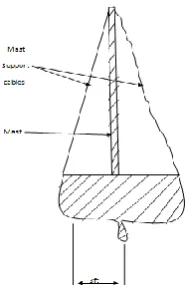
Application in engineering problem.

Problem: A cross section of a racing sailboat is shown in fig .4.1(a). Wind forces (f ) exerted per foot of must from the sails very as a function of distance above the deck of the boat (z),as in Fig.4.1(b). Calculate the tensile force T in the mast support cable, assuming that the right support cable in completely slack and the must joins the deck in a manner that transmits horizontal or vertical forces but on moments. Assume remains vertical.

(b)

Fig( 4.1) wind forces (f ) exerted per foot of must from the sails very as a function of distance above the deck of the boat

Fig( 4.2)Forces exerted on the mast of a sailboat

30

2 /30 0

200 5

z z

F e dz

z



 

 _{ }



 



The nonlinear integral is difficult to evaluate analytically. Therefore, it is convenient to employ numerical approaches such as Simson’s rule and the trapezoidal rule for this problem.This is accomplished by calculating f(z) for various values of z.

Description: values of f(z) for a step size 3 ft that provide data for the trapezoidal rule and Simpson’s 1/3 rule.

Z,ft 0 3 6 9 12 15 18 21 24 27 30

f(z),lb/ft 0 61.40 73.13 70.56 63.43 55.18 47.14 39.83 33.42 27.89 23.20 Solution: Value of F computed on the basis of various version of the trapezoidal rule and Simpson’s 1/3 rule.

Table( 6) Trapezoidal Rule

Step size, ft Segments F,lb

15 2 1001.7

10 3 1222.3

6 5 1372.3

3 10 1450.8

1 30 1477.1

.5 60 1479.7

.25 120 1480.3

.1 300 1480.5

.05 600 1480.6

Table( 7) Simpson 1/3 Rule

Step size, ft Segments F,lb

15 2 1219.6

5 6 1462.9

3 10 1476.9

1 30 1480.5

Now we are applying the Romberg's method of integration for the results obtained by the above methods.

Result obtained by Romberg's method of integration: I(h)=1477.1 I(h/2)=1479.7 I(h/4)=1480.3 I(h,h/2)=1477.3 I(h/2,h/4)=1480.86 I(h,h/2,h/4)=1481.34 Conclusion

We have seen that in situations where it is impossible to know the function governing some phenomenon exactly, it is still possible to derive a reasonable estimate for the integral of the function based on data points. The idea is to choose a model function going through the data points and integrate the model function. The definition of an integral as a limit of Riemann sums shows that if we chose enough data points, the integral of the model function converges to the integral of the unknown function; so theoretically, numerical integration is on solid ground. We have also seen that there are many practical factors that influence how well numerical integration works. Simple model functions may not emulate the behavior of the unknown function well. Complicated model functions are hard to work with. Problems with the number of data points, or the way in which the data was collected can have a major impact, and while we have explored some simple ways of estimating how accurate a particular numerical integral will be, this can be quite complicated in general.

REFERENCES

Adimy, Mostafa, Oscar Angulo, Fabien Crauste, Juan C. López-Marcos. 2008. “Numerical integration of a mathematical

model of hematopoietic stem cell dynamics.” Computers

& Mathematics with Applications 56(3): 594-606.

Gourdon, Xavier and Pascal Sebah. 2002. Introduction on

Bernoulli's numbers.

Hadjifotinou, K.G. 2002. “Numerical integration of the variational equations of satellite orbits.” Planetary and Space Science 50(4): 361-369.

Lorenzini, R. and L. Passoni. 1999. “Test of numerical methods for the integration of kinetic equations in tropospheric

chemistry.” Computer Physics Communications 117(3):

241-249.

Mai, Enrico and Robin Geyer. 2013.

“Numerical Orbit Integration based on Lie Series with

Use of Parallel Computing Techniques.” Advances in

Space Research (In Press, Accepted Manuscript, Available online 21 October 2013)

Meng, Zhao-Liang and Zhong-Xuan Luo. 2011. “The construction of numerical integration rules of degree

three for product regions.” Applied Mathematics and

Computation 218(5): 2036-2043.

Papoulis, A. 1984. Probability, Random Variables, and

Stochastic Processes. 2nd ed. New York: McGraw-Hill, pp. 147-148.

Petrovskaya, Natalia and Ezio Venturino. 2011. “Numerical

integration of sparsely sampled data.” Simulation

Modeling Practice and Theory 19(9): 1860-1872

Sladek, V., J. Sladek, and M. Tanaka. 2001. “Numerical integration of logarithmic and nearly logarithmic

singularity in BEMs.” Applied Mathematical Modelling

Vardi, I. 1991. "The Euler-Maclaurin Formula." In Computational Recreations in Mathematica, 159-163. Reading, MA: Addison-Wesley.

Watson, G. N. 1928. "Theorems Stated by Ramanujan (IV): Theorems on Approximate Integration and Summation of Series." J. London Math. Soc. 3: 282-289.

Weisstein, Eric W. "Euler–Maclaurin Integration

Formulas." MathWorld.

Whittaker, E. T. and Robinson, G. 1967. "The Euler-Maclaurin Formula." §67 In The Calculus of Observations: A Treatise on Numerical Mathematics, 134-136. 4th ed. New York: Dover.

Whittaker, E. T. and Watson, G. N. 1990. "The Euler-Maclaurin Expansion." In A Course in Modern Analysis, 127-128. 4th ed. Cambridge, England: Cambridge University Press.

Xiu, Dongbin. 2008. “Numerical integration formulas of degree

two.” Applied Numerical Mathematics 58(10):