Beginning Python Visualization.pdf

Shai Vaingast

Beginning Python

Visualization

All rights reserved. No part of this work may be reproduced or transmitted in any form or by any means, electronic or mechanical, including photocopying, recording, or by any information storage or retrieval system, without the prior written permission of the copyright owner and the publisher.

ISBN-13 (pbk): 978-1-4302-1843-2 ISBN-13 (electronic): 978-1-4302-1844-9

Printed and bound in the United States of America 9 8 7 6 5 4 3 2 1

Trademarked names may appear in this book. Rather than use a trademark symbol with every occurrence of a trademarked name, we use the names only in an editorial fashion and to the benefit of the trademark owner, with no intention of infringement of the trademark.

Lead Editors: Frank Pohlmann, Michelle Lowman Technical Reviewer: C. Titus Brown

Editorial Board: Clay Andres, Steve Anglin, Mark Beckner, Ewan Buckingham, Tony Campbell, Gary Cornell, Jonathan Gennick, Michelle Lowman, Matthew Moodie, Jeffrey Pepper, Frank Pohlmann, Ben Renow-Clarke, Dominic Shakeshaft, Matt Wade, Tom Welsh Project Manager: Kylie Johnston

Copy Editor: Ami Knox

Associate Production Director: Kari Brooks-Copony Production Editor: Kelly Winquist

Compositor: Dina Quan Proofreader: Liz Welch Indexer: Julie Grady Artist: April Milne

Cover Designer: Kurt Krames

Manufacturing Director: Tom Debolski

Distributed to the book trade worldwide by Springer-Verlag New York, Inc., 233 Spring Street, 6th Floor, New York, NY 10013. Phone 1-800-SPRINGER, fax 201-348-4505, e-mail kn`ano)ju<olnejcan)o^i*_ki, or visitdppl6++sss*olnejcankjheja*_ki.

For information on translations, please contact Apress directly at 2855 Telegraph Avenue, Suite 600, Berkeley, CA 94705. Phone 510-549-5930, fax 510-549-5939, e-mail ejbk<]lnaoo*_ki, or visit dppl6++sss* ]lnaoo*_ki.

Apress and friends of ED books may be purchased in bulk for academic, corporate, or promotional use. eBook versions and licenses are also available for most titles. For more information, reference our Special Bulk Sales–eBook Licensing web page at dppl6++sss*]lnaoo*_ki+ejbk+^qhgo]hao.

The information in this book is distributed on an “as is” basis, without warranty. Although every precau-tion has been taken in the preparaprecau-tion of this work, neither the author(s) nor Apress shall have any liability to any person or entity with respect to any loss or damage caused or alleged to be caused directly or indi-rectly by the information contained in this work.

v

Contents at a Glance

About the Author

. . . xv

About the Technical Reviewer

. . . xvi

Acknowledgments

. . . xvii

Introduction

. . . xviii

CHAPTER 1

Navigating the World of Data Visualization

. . . 1

CHAPTER 2

The Environment

. . . 31

CHAPTER 3

Python for Programmers

. . . 53

CHAPTER 4

Data Organization

. . . 101

CHAPTER 5

Processing Text Files

. . . 135

CHAPTER 6

Graphs and Plots

. . . 183

CHAPTER 7

Math Games

. . . 221

CHAPTER 8

Science and Visualization

. . . 249

CHAPTER 9

Image Processing

. . . 285

CHAPTER 10

Advanced File Processing

. . . 319

APPENDIX

Additional Source Listing

. . . 343

vii

Contents

About the Author

. . . xv

About the Technical Reviewer

. . . xvi

Acknowledgments

. . . xvii

Introduction

. . . xviii

CHAPTER 1

Navigating the World of Data Visualization

. . . 1

Gathering Data

. . . 2

Case Study: GPS Data

. . . 2

Scanning Serial Ports

. . . 3

Recording GPS Data

. . . 5

Data Organization

. . . 6

File Format

. . . 6

File Naming Conventions

. . . 7

Data Location

. . . 7

Data Analysis

. . . 8

Walking Directories

. . . 8

Reading CSV Files

. . . 9

Analyzing GPS Data

. . . 12

Extracting GPS Data

. . . 14

Data Visualization

. . . 17

GPS Location Plot

. . . 18

Annotating the Graph

. . . 20

Velocity Plot

. . . 22

Subplots

. . . 23

Text

. . . 23

Tying It All Together

. . . 25

CHAPTER 2

The Environment

. . . 31

Operating Systems

. . . 32

GNU/Linux

. . . 32

Windows

. . . 33

Choosing an Operating System

. . . 35

Then Again, Why Choose? Using Several Operating Systems

. . . 36

The Python Environment

. . . 37

Versions

. . . 37

Python

. . . 38

Python Integrated Development Environments

. . . 39

Scientific Computing

. . . 41

Plotting

. . . 42

Image Processing

. . . 43

Additional Python Packages

. . . 43

Installation Summary

. . . 44

Additional Applications

. . . 45

Editors

. . . 45

A Short List of Text Editors

. . . 47

Spreadsheets

. . . 48

Word Processors

. . . 48

Image Viewers

. . . 49

Version Control Systems

. . . 49

Licensing

. . . 51

Final Notes and References

. . . 52

CHAPTER 3

Python for Programmers

. . . 53

What Is Python?

. . . 53

Interactive Python

. . . 54

Invoking Python

. . . 54

Entering Commands

. . . 55

The Interactive Help System

. . . 56

Moving Around

. . . 57

Running Scripts

. . . 58

Data Types

. . . 60

Numbers

. . . 60

Strings

. . . 65

Data Structures

. . . 68

Lists

. . . 69

Tuples

. . . 72

Dictionaries

. . . 74

Sets

. . . 78

Variables

. . . 80

Statements

. . . 81

Printing

. . . 81

User Input

. . . 84

Comments

. . . 85

Flow Control

. . . 85

Some Built-in Functions

. . . 92

Defining Functions

. . . 93

Generators

. . . 94

Generator Expressions

. . . 95

Object-Oriented Programming

. . . 96

Modules and Packages

. . . 97

The import Statement

. . . 98

Modules Installed in a System

. . . 99

The dir Statement

. . . 99

Final Notes and References

. . . 99

CHAPTER 4

Data Organization

. . . 101

File Name Conventions

. . . 102

Date and Time in a File Name

. . . 102

Useful File Name Titles

. . . 104

File Name Extensions

. . . 104

In Conclusion

. . . 105

Other Schemes

. . . 107

File Formats

. . . 108

CSV File Format

. . . 109

Binary Files

. . . 117

Readme Files

. . . 123

INI Files

. . . 123

XML

. . . 125

Other File Formats

. . . 126

Locating Data Files

. . . 126

Organization into Directories

. . . 126

Searching for Files

. . . 127

Catalogs

. . . 131

Files vs. a Database

. . . 133

Final Notes and References

. . . 134

CHAPTER 5

Processing Text Files

. . . 135

Text and Strings

. . . 136

Splitting Text

. . . 136

Joining Strings

. . . 137

Converting Strings to Numbers

. . . 137

Find and Replace

. . . 143

Stripping Strings

. . . 144

String Formatting

. . . 145

String Conditionals

. . . 146

More on Strings

. . . 147

Files

. . . 147

Opening a File

. . . 147

Closing a File

. . . 148

Writing Text

. . . 148

Reading Text

. . . 149

Working with Text Files

. . . 150

Example: Character, Word, and Line Count

. . . 151

Example: head and tail

. . . 152

Example: Splitting and Combining Files

. . . 153

Example: Searching Inside a Text File

. . . 155

Example: Working with Comments

. . . 156

Example: Extracting Numbers from a Text File

. . . 157

CSV Files

. . . 159

The csv Module

. . . 159

The csv.reader Object

. . . 160

The csv.writer Object

. . . 161

More csv Functionality

. . . 161

DictReader and DictWriter Objects

. . . 162

Date and Time

. . . 163

Time Module

. . . 164

The struct_time Tuple

. . . 165

Parsing and Formatting Date and Time

. . . 165

The Epoch: “Linearizing” the Time Base

. . . 168

Regular Expressions

. . . 173

Regular Expression Patterns

. . . 173

Special Sequences

. . . 175

Alternatives

. . . 175

Ranges

. . . 175

When to Use Regular Expressions

. . . 175

Internationalization and Localization

. . . 176

Locale

. . . 177

Unicode Strings

. . . 178

Final Notes and References

. . . 181

CHAPTER 6

Graphs and Plots

. . . 183

The Matplotlib Package

. . . 183

Interactive Graphs vs. Image Files

. . . 184

Interactive Graphs

. . . 185

Saving Graphs to Files

. . . 187

Plotting Graphs

. . . 189

Lines and Markers

. . . 189

Plotting Several Graphs on One Figure

. . . 191

Line Widths and Marker Sizes

. . . 192

Colors

. . . 193

Controlling the Graph

. . . 194

Axis

. . . 194

Grid and Ticks

. . . 195

Subplots

. . . 196

Erasing the Graph

. . . 197

Adding Text

. . . 197

Title

. . . 198

Axis Labels and Legend

. . . 198

Text Rendering

. . . 199

Mathematical Symbols and Expressions

. . . 200

More Graph Types

. . . 201

Bar Charts

. . . 201

Histograms

. . . 204

Pie Charts

. . . 206

Logarithmic Plots

. . . 207

Polar Plots

. . . 208

Stem Plots

. . . 209

Getting and Setting Values

. . . 213

Setting Figure and Axis Parameters

. . . 215

Patches

. . . 217

Example: Adding Arrows to a Graph

. . . 218

Example: Some Other Patches

. . . 219

Final Notes and References

. . . 220

CHAPTER 7

Math Games

. . . 221

Modules math and cmath

. . . 221

Example: A Newton Fractal

. . . 224

Module random

. . . 228

Using random to Solve Probability Questions

. . . 229

Random Sequences

. . . 232

Module NumPy

. . . 233

Array Creation

. . . 234

Slicing, Indexing, and Reshaping

. . . 235

N-Dimensional Arrays

. . . 236

Math Functions

. . . 239

Array Methods and Properties

. . . 241

Other Useful Array Functions

. . . 247

Final Notes and References

. . . 247

CHAPTER 8

Science and Visualization

. . . 249

Finding Your Way: Variables and Functions

. . . 250

SciPy

. . . 250

Linear Algebra

. . . 251

Solving a System of Linear Equations

. . . 251

Vector and Matrix Operations

. . . 252

Matrix Decomposition

. . . 253

Additional Linear Algebra Functionality

. . . 254

Numerical Integration

. . . 254

More Integration Methods

. . . 257

Interpolation and Curve Fitting

. . . 258

Piecewise Linear Interpolation

. . . 258

Polynomials

. . . 260

Uses of Polynomials

. . . 261

Solving Nonlinear Equations

. . . 267

Special Functions

. . . 268

Signal Processing

. . . 268

Functions where, select, and find

. . . 269

Functions diff and split

. . . 273

Waveforms

. . . 274

Fourier Transform

. . . 275

Example: FFT of a Sampled Cosine Wave

. . . 276

Window Functions

. . . 277

Filtering

. . . 279

Filter Design

. . . 279

Example: Heart-Rate Monitor

. . . 281

Example: Moving Average

. . . 283

Final Notes and References

. . . 284

CHAPTER 9

Image Processing

. . . 285

Reading, Writing, and Displaying Images

. . . 286

Reading Images from File

. . . 286

Image Attributes

. . . 287

Displaying Images

. . . 288

Converting File Formats

. . . 289

Image Manipulation

. . . 291

Creating New Images

. . . 291

Copy and Paste

. . . 292

Crop and Resize

. . . 292

Rotate

. . . 293

Image Annotation

. . . 294

Annotating with Geometrical Shapes

. . . 294

Text Annotations

. . . 295

Image Processing

. . . 300

Matrix Representation and Colors

. . . 300

Example: Counting Objects (Five Parts)

. . . 303

Image Arithmetic

. . . 312

Image Filtering

. . . 315

CHAPTER 10

Advanced File Processing

. . . 319

Binary Files and Random Access

. . . 319

Example: Reading the Nth Field

. . . 321

Example: Efficient Tail Implementation

. . . 322

Example: Creating a Fixed-Size File

. . . 323

Example: Recording Time-Based Binary Data

. . . 323

Object Serialization

. . . 325

The Pickle Module

. . . 325

Command-Line Parameters

. . . 327

argv

. . . 327

Example: Creating a Fixed-Size File (Stand-Alone Script)

. . . 328

OptParse Module

. . . 329

The FileInput Module

. . . 332

File and Directory Manipulation

. . . 333

Module glob

. . . 334

Additional os Module Functionality

. . . 334

Additional os.path Module Functionality

. . . 335

Module shutil

. . . 336

File Compression

. . . 337

Example: A Compressed tar File

. . . 338

Comparing Files

. . . 339

Module filecmp

. . . 339

Module difflib

. . . 341

Final Notes and References

. . . 342

APPENDIX

Additional Source Listing

. . . 343

Nudge Subplots

. . . 343

Magic Square Arrows

. . . 345

Fractal Function Source Code

. . . 347

xv

About the Author

xvi

About the Technical Reviewer

xvii

Acknowledgments

xviii

Introduction

I

was always drawn to math and computers, ever since I was a kid playing computer games on my Sinclair ZX81. When I attended university, I had a special interest in numerical analy-sis, a field that I felt combines math and computers ideally. During my career, I learned of MATLAB, widely popular for digital signal processing, numerical analysis, and feedback and control. MATLAB’s strong suits include a high-level programming language, excellent graph-ing capabilities, and numerous packages from almost every imaginable engineergraph-ing field. But I found that MATLAB wasn’t enough. I worked with very large files and needed the ability to manipulate both text and data. So I combined Perl, AWK, and Bash scripts to write programs that automate data analysis and visualization. And along the way, I’ve developed practices and ideas involving the organization of data—for example, ways to ensure file names are unique and self-explanatory.

With the increasing popularity of the Internet, I learned of GNU/Linux and the open source movement. I made an effort to use open source software whenever possible, and so I’ve learned of GNU-Octave and gnuplot, which together provide excellent scientific computing functionality. That fit well on my Linux machine: Bash scripts, Perl and AWK, GNU-Octave and gnuplot.

Knowing I was interested in programming languages and open source software, a friend suggested I give Python a try. My first impression was that it’s just another programming lan-guage: I can do most anything I need with Perl and Bash, resorting to C/C++ if things got hairy. And I’d still need GNU-Octave and gnuplot, so what’s to gain? Eventually, I did learn Python and discovered that it is far better than my collection of tools. Python provides something that is extremely appealing: it’s a one-stop shop—you can do it all in Python.

I’ve shared my enthusiasm with friends and colleagues. Many who expressed interest with the ideas of data processing and visualization would ask, “Can you recommend a book that teaches the ideas you’re preaching?” And I would tell them, “Of course, numerous books cover this subject!” But they didn’t want numerous books, just one, with information distilled to focus on data analysis and visualization. I realized there wasn’t such a title, and this was how the idea for this book originated.

Who This Book Is For

s 'RADUATEAND0H$STUDENTSINEXACTANDNATURALSCIENCESPHYSICSBIOLOGYANDCHEM-istry) working on their thesis, dealing with large experimental data sets. The book also appeals to students working on purely theoretical projects, as they require simulations and means to analyze the results.

s 2$ENGINEERSINTHEFIELDSOFELECTRICALENGINEERING%% MECHANICALENGINEERINGAND chemical engineering: engineers working with large sets of data from multiple sources. In EE more specifically, signal processing engineers, communication engineers, and systems engineers will find the book appealing.

s 0ROGRAMMERSANDCOMPUTERENTHUSIASTSUNFAMILIARWITH0YTHONANDTHE'.5,INUX world, willing to dive into a new world of tools.

s (OBBYASTRONOMERSANDOTHERHOBBYISTSWHODEALWITHDATAANDAREINTERESTEDINUSING Python to support their hobby.

The book can be appealing to these groups for different reasons. For scientists and engi-neers, the book provides the means to be more productive in their work, without investing a considerable amount of time learning new tools and programs that constantly change. For programmers and computer enthusiasts, the book can serve as an appetizer, opening up their world to Python. And because of the unique approach presented here, they might share the enthusiasm the author has for this wonderful software world. Perhaps it will even entice them to be part of the large and growing open source community, sharing their own code.

It is assumed that the reader does have minimal proficiency with a computer; namely he or she must know how to manipulate files, install applications, view and edit files, and use applications to generate reports and presentations. Background in numerical analysis, signal processing, and image processing, as well as programming, is of help, but not required.

This book does not intend to serve as an encyclopedia of programming in Python and the covered packages; nor does it try to be complete. It serves as an introduction to data analysis and visualization in Python and covers most of the topics associated with that field.

How This Book Is Structured

The book is designed so that you can easily skip back and forth as you engage topics.

Chapter 1 is a case study introducing the topics discussed throughout the book: data anal-ysis, data management, and, of course, data visualization. The case study involves reading GPS data, analyzing it, and plotting it along with relevant annotations (direction of travel, speed, etc.). A fully functional Python script will be built from the ground up, complemented with lots of explanations. The fruit of our work will be an eye-catching GPS route.

If you’re new to data analysis and visualization, consider reading Chapter 2 first. The chapter describes how to set up a development environment to perform the tasks associated with data analysis and visualization in Python, including the selection of an OS, installing Python, and installing third-party packages.

Regardless of your Python programming experience, I highly encourage you to read Chap-ter 4 before proceeding to the next chapChap-ters. Organization is the key to successful data analysis and visualization. This chapter covers organizing data files, pros and cons of different file formats, file naming conventions, finding data files, and automating file creation. The ideas in Chapter 4 are used throughout the book.

From here on out you have several options. If you intend to process text and data files, proceed to Chapter 5. Chapter 5 covers text files from all aspects: I/O operations, string pro-cessing, the csv module, regular expressions, and localization and internationalization. If Chapter 5 leaves you wanting to know more about file processing, proceed to Chapter 10. Chapter 10 includes advanced file processing topics: binary files, command-line arguments, file and directory manipulation, and more. Both Chapters 5 and 10 are complemented with numerous examples.

If graphs and plots are your heart’s desire, skip directly to Chapter 6. In Chapter 6 I exam-ine matplotlib and explore its capabilities.

If you’re interested in the numerical aspects of data, it is advised you read Chapter 7 first. Chapter 7 discusses the basic building blocks for scientific computing. Chapter 8 builds on Chapter 7 and includes more advanced topics such as numerical analysis and signal processing.

Image processing is an important aspect of data processing. Chapter 9 deals with tools available as part of the Python Imaging Library (PIL) package and shows how to further expand the package and perform more complex image processing tasks.

Chapter 10 covers advanced file processing topics including binary files and random access, object serialization, command-line parameters, file compression, and more.

Finally, the Appendix provides additional source code listings used in the book.

Downloading the Code

The source code for this book is available to readers at sss*]lnaoo*_ki in the Source Code sec-tion of this book’s home page. Please feel free to visit the Apress web site and download all the code there. You can also check for errata and find related titles from Apress.

Navigating the World of Data

Visualization

A Case Study

A

s an engineer, I work with data all the time. I parse log files, analyze data, estimate values, and compare the results with theory. Things don’t always add up. So I double-check my analy-sis, perform more calculations, or run simulations to better understand the results. I refer to previous work because the ideas are similar or sometimes because they’re dissimilar. I look at the graphs and realize I’m missing some crucial information. So I add the missing data, but it’s noisy and needs filtering. Eventually, I realize my implementation of the algorithm is poor or that there is a better algorithm with better results, and so back to square one. It’s an iterative process: tweak, test, tweak again until I’m satisfied with the results.

Those are the tasks surrounding research and development (R&D) work. And to be honest, there’s no systematic method. Most of the time, research is organized chaos. The emphasis, however, should be on organized, not chaos. Data should be analyzed and presented in a clear and coherent manner. Sources for graphs well understood and verified to be accurate. Algorithms tested and proven to be working as intended. The system should be flexible. Intro-ducing new ideas and challenging previous methods should be easy and testing new ideas on current data fast and efficient.

In this book I will attempt to address all the topics associated with data processing and visualization: managing files and directories, reading files of varying formats, performing signal processing and numerical analysis in a high-level programming language similar to MATLAB and GNU-Octave, and teaching you Python, a rich and powerful programming lan-guage, along the way.

In a nutshell, Beginning Python Visualization deals with the processing, analysis, manipu-lation, and visualization of data using the Python programming language. The book covers the following:

s &UNDAMENTALSOFTHE0YTHONPROGRAMMINGLANGUAGEREQUIREDFORDATAANALYSISAND visualization

s $ATAFILESFORMATANDORGANIZATIONASWELLASMETHODSANDGUIDELINESFORSELECTINGFILE formats and storing and organizing data to enable fast, efficient data processing

s 2EADILYAVAILABLE0YTHONPACKAGESFORNUMERICALANALYSISSIGNALANDIMAGEPROCESSING graphing and plotting, and more

Gathering Data

We spend a considerable time recording and analyzing data. Data is stored in various formats depending on the tools used to collect it, the nature of the data (e.g., pictures vs. sampled analog data), the application that will later process the data, and personal preferences. Data files are of varying sizes; some are very large, others are smaller but in larger quantities. Data ORGANIZATIONADDSANOTHERLEVELOFCOMPLEXITY&ILESCANBESTOREDINDIRECTORIESACCORDINGTO date, grouped together in one big directory or in a database, or adhere to a different scheme altogether. Typically, the number of data files or the amount of data per file is too large to allow skimming or browsing with an editor or viewer. Methods and tools are required to find the data and analyze it to produce meaningful results.

Case Study: GPS Data

You just got a USB GPS receiver for your birthday! You’d like to analyze GPS data and find out how often you exceed the speed limit and how much time you spend in traffic. You’d like to track data over a year, or even longer.

Some hardware background: most USB GPS receivers behave as serial ports (this is also true for Bluetooth GPS devices). What this means is that once a GPS is connected, and assum-ing it’s installed properly, readassum-ing GPS data is as simple as openassum-ing the COM port associated with the GPS and reading the values. GPS values are typically clear text values: numbers and text. Of course, if you’re planning on recording data from your car, it would make a lot of sense to hook it up to a laptop rather than a desktop.

7EWOULDLIKETORECORDANALYZEANDVISUALIZETHE'03DATAIN0YTHON&IRSTTHINGSFIRST recording GPS data.

N

Note

If you wish to follow along with the remainder of the chapter by means of issuing the commands yourself and viewing the results, you might first want to refer to Chapter 2 and set up Python on your system. That being said, it’s not necessary, and you can follow along to get an understanding of the book and its purpose. In fact, I encourage you to come back to this chapter and read it again after you’ve had more expe-rience with Python.

interpreted programming languages is that it’s easy to run them interactively. That is, perform a command, examine the results, perform more commands, and examine more results, and so on. The ability to run Python interactively is very useful, and it allows you to examine topics as you learn them.

It’s also possible to run Python scripts, that is, noninteractively, and there are several ways to do that. You can run scripts from the interactive Python prompt by issuing the command

ata_beha$#o_nelpj]ia*lu#%. Or you can enter lupdkjo_nelpj]ia*lu at the command-line interface of your operating system. If you’re using IPython, you can issue the command nqj o_nelpj]ia*lu instead; and if you’re running IDLE, the Python GUI, you can open the script ANDPRESS&TOEXECUTEIT4HE*lu extension is a common convention that distinguishes Python scripts from other files.

Back to recording GPS data. To be able to access the serial port from Python, we’ll be using the pySerial module. PySerial, as the name suggests, allows seamless access to serial ports. To use pySerial we must first read the module to memory, that is, import it using the

eilknp command. If all goes well, we’ll be presented with the Python prompt again.

:::eilknpoane]h

N

Note

To distinguish between interactive sessions and Python scripts, when code starts with :::, it means that the code was run on Python interactively. In case the ellipsis symbol (***) appears, it means that this is a continuation of a previously interactively entered command. Lines of text following the symbols ***

or::: is Python’s response to the issued command. A code listing that does not start with ::: is a script written in an editor, and in order to execute it you will have to save it under o_nelpj]ia*lu (or some other name) and execute it as described previously.

Scanning Serial Ports

Next, we need to find the serial port parameters: the baud rate and the port number. The baud rate is a GPS parameter, so it’s best to consult the GPS manual (not to worry if you can’t find this information, I’ll discuss later how to “guess” what it is). As for the port number, this is determined by your operating system. If you’re not sure how to find the port number, or if the port number keeps changing when you plug and unplug your GPS, you can use the short pro-gram in Listing 1-1 to identify active serial ports.

Listing 1-1. Scanning Serial Ports with o_]jlknp*lu eilknpoane]h

bkqj`9B]hoa bkneejn]jca$20%6 pnu6

oan9oane]h*Oane]h$e% oan*_hkoa$%

at_alpoane]h*oane]hqpeh*Oane]hAt_alpekj6 l]oo

ebjkpbkqj`6

lnejpJklknpobkqj`(i]gaoqnaCLOeo_kjja_pa`*

N

Note

Short programs are typically referred to asscripts.

Runo_]jlknp*lu and note the result:

:::ata_beha$#o_]jlknp*lu#% Bkqj`?KI1

This is a rather QUICKINTRODUCTIONTO0YTHON&IRSTLETSDISSECTo_]jlknp*lu line by line. The first line, eilknpoane]h, loads the pySerial module. We then assign to the Boolean vari-ablebkqj` the value B]hoa; this variable will be used as an indication of whether a serial port was found or not. We proceed with the bkn loop: the loop goes over the values between , and

2/ as implied by n]jca$20% (most systems have less than 64 virtual COM ports). The function

n]jca$J% returns a list of values from , to J)-. Our approach to seeing what ports are available is rather simple: try and open the port, and if all goes well, that port is a candidate. If it was not possible to open the port, just ignore that port. And so this is exactly how it’s coded!

4HISISACOMMONMOTTOIN0YTHON)TS%ASIERTO!SK&ORGIVENESSTHAN0ERMISSIONOR %!&04HEIDEAISTHIS4RYANDPERFORMANOPERATION)FALLGOESWELLGREAT)FNOTHANDLEIT with the at_alp clause, or more figuratively, ask forgiveness. This is eloquently coded with the

pnu/at_alp mechanism.

In our case, the function that’s most likely to fail (raise an exception) is the one that tries to open a nonexistent port: oan9oane]h*Oane]h$e%. The function Oane]h$% is part of the serial module (notice case sensitivity). To access functions within modules, you specify the mod-ule name, dot (*), and the function name. So to call the function Oane]h$% within the module serial, write oane]h*Oane]h$%. The function Oane]h$% takes one parameter: the port number. Python, like C, starts counting at 0, so remember to subtract 1 from your virtual COM port WHENPASSINGAPARAMETERTOTHEFUNCTION-Y'03TURNEDOUTTOBECONNECTEDTO#/-SOA call to oane]h*Oane]h$0% will allow me access to the GPS. If the port is successfully opened, no exception is raised, and the opened port is associated with the variableoan.

The next line in thepnu block, oan*_hkoa$%, tries to close the port. Closing the port renders it accessible to other applications, including your own. If you neglect to close the port, Python will close it for you once the variable associated with it, oan, is no longer in use. We also print out a message saying the port is a good candidate and set the bkqj` flag toPnqa.

If the block of commands under pnu fails, the block of commands under at_alp is exe-cuted assuming the at_alp condition is met. In our case, if an exception occurred, and if the exception is of type oane]h*oane]hqpeh*Oane]hAt_alpekj, which means the port could not be opened, we want to simply disregard it. This is done using the l]oo statement, which does nothing.

N

Note

The indentation (tabs) in Python is important because it groups commands together. This is also true when using Python in an interactive mode. All lines with the same indentation are considered one block. Python’s indentation is equivalent to C/C++ curly braces—wy.

Recording GPS Data

Let’s start gathering data. Enter code in Listing 1-2 and record it in the file na_kn`[clo*lu.

Listing 1-2. na_kn`[clo*lu eilknppeia(oane]h

_d]jcapdaoal]n]iapanopkukqnCLOl]n]iapano oan9oane]h*Oane]h$0%

oan*^]q`n]pa904,,

bip9**+`]p]+CLO)!0`)!,.`)!,.`)!,.`)!,.`)!,.`*_or

behaj]ia9bip!peia*hk_]hpeia$%W,62Y b9klaj$behaj]ia(#s^#%

sdehaPnqa6

heja9oan*na]`heja$% b*snepa$heja%

lnejpheja(

This time, we’ve imported another module: time. The time module provides access to date and time functions, and we’ll use those to name our GPS data files. We also introduce an important notion here, comments! Comments in Python are denoted by the sign and are similar to C++ double slash notation, ++. Everything from that point onward is considered a remark. If the sign is at the beginning of a line, then the entire line is a remark, usually describing the next line or block of code. The exception to the sign indicating a remark is if it is quoted inside a string, as follows: .

Don’t forget to change the port number to point at your serial port (minus 1) and set the proper baud rate. Determining the baud rate is not complex either—best to consult the manual. Mine turned out to be 4800, but if you’re not sure, you can tweak this parameter. The scriptna_kn`[clo*lu will print the output from the GPS on screen so you can change the baud rate value (in multiples of 2, for example 4800, 9600, and so on) until you see some meaningful results (i.e., text and numbers).

Runningna_kn`[clo*lu (I’ll get to how it works soon) yields GPS data:

:::ata_beha$#na_kn`[clo*lu#%

CLNI?(-0,,1/*,,(=(0010*-30,(J(,5/.1*,-0/(S(,,,*,(-.4*3(/,,1,4(,,-*-(A(=&.A CLCC=(-0,,1/*,,(0010*-30,(J(,5/.1*,-0/(S(-(,5(,-*-(,,.45*4(I(),/,*3(I((&1A CLCO=(=(/(.-(-1(-4(.0(.2(.5(,2(..((,/(((,.*,(,-*-(,-*3&,0

CLNI?(-0,,10*,,(=(0010*-30,(J(,5/.1*,-0/(S(,,,*,(-.4*3(/,,1,4(,,-*-(A(=&.5 CLCC=(-0,,10*,,(0010*-30,(J(,5/.1*,-0/(S(-(,5(,-*-(,,.45*4(I(),/,*3(I((&15 CLCO=(=(/(.-(-1(-4(.0(.2(.5(,2(..((,/(((,.*,(,-*-(,-*3&,0

Data is being recorded to file as it is displayed. When you wish to stop viewing and record-ing GPS data, press Ctrl+C. If you’re runnrecord-ing in an interactive Python, once you issue Ctrl+C, be sure to close the serial port, or you won’t be able to rerun the script na_kn`[clo*lu. To close the port, issue the following command:

:::oan*_hkoa$%

It’s also a good idea to close the file:

:::b*_hkoa$%

Let’s turn back so I can explain how na_kn`[clo*lu works. The heart of the script lies in the following lines of code:

sdehaPnqa6

heja9oan*na]`heja$% b*snepa$heja%

lnejpheja(

This is a straightforward implementation. The first line, sdehaPnqa6, instructs that the following block should be run indefinitely, that is, in an infinite loop. That’s why you need to press Ctrl+C to stop recording. The next three lines are then executed continuously. What we do is read a line of text from the serial port, store it to file, and print it to screen. Reading GPS data is carried out by the command heja9oan*na]`heja$%. Writing that data to a file for later processing is done by b*snepa$heja%. Printing the data to screen so the user has some visual feedback is done with lnejpheja(. The reason for the comma following heja is to suppress an extra line break.

Data Organization

Let’s turn to selecting file format, file naming conventions, and data location. Now there isn’t a good solution that fits all, but the methodologies and ideas are simple. The method I’ll use here is based on file names. I’ll show you how to name data files in a way that lends itself easily to automatic processing later on.

File Format

A file format is ASETOFRULESDESCRIBINGTHECONTENTSOFAFILE&ORTHE'03PROBLEMWELLCHOOSE the Comma Separated Values (CSV) file format. CSV files are text files with values separated by COMMAS&OREXAMPLE

CLCOR(/(.(-.(,2(0/(,52(/3(,3(0-(.5-(/4(-2(/5(,1.(/.(.3(/0(.5-(/0&32 CLCOR(/(/(-.(-5(.2(-1.(/1(,4(,2(.4,((-,(,,(//3((,,(,,(,,,(&30

CSV is a popular format recognized by most spreadsheets and database applications and, of course, text editors, seeing as they’re really just text files. As it turns out, the data the GPS outputs is already comma separated, so all that’s required is to save this information to a file, as is.

File Naming Conventions

We turn to selecting PROPERFILENAMESFOROURDATAFILES&ILENAMESSHOULDBEUNIQUESOTHAT FILESWONTBEACCIDENTALLYOVERWRITTEN&ILENAMESSHOULDBEDESCRIPTIVETHATISTELLUSSOME-thing about the contents. Lastly, we’d like the file name extension to tell us how to view the file. The latter is typically achieved by selecting a proper extension, in our case, *_or. Here are the naming conventions I chose for this example:

s &ILENAMESHOLDING'03DATAWILLSTARTWITHTHETEXTh'03v

s .EXTISTHEDATEANDTIMEIN)3/FORMATWITHTHESEPARATINGCOLONSOMITTEDANDA hyphen between the date and time: YYYY-mm-dd-HH-MM-SS, where YYYY stands for year, mm for month, dd for day, HH for hours, MM for minutes, and SS for seconds. In case a value is one digit and two digits are required, values will be padded with zeros, FOREXAMPLETHEMONTHOF-AYWILLBEDENOTEDBYNOT&ORADDITIONALINFORMATION regarding the ISO format, refer to ISO 8601, “Data elements and interchange formats— Information interchange—Representation of dates and times” (dppl6++sss*eok*knc).

s !LLFILESWILLHAVEA*_or extension.

&OLLOWINGTHESECONVENTIONSAFILENAMEMIGHTLOOKlike this:

CLO).,,4),1)/,),5)-,)1.*_or

Data Location

This is where we store data files:

s !LLDATAFILESARESTOREDINDIRECTORY`]p]. All scripts are stored in directory on_. Both directories are under the same parent directory ?d-. So a relative path from on_ to `]p]

is**+`]p].

s )TSAGOODIDEAto also add a Na]`ia*ptp file. Readme files are clear text files describing the contents of a directory, in as much detail as deemed reasonable: the data source, data acquisition system, person in charge of data gathering, reason for gathering the data, and so on. Here’s an example:

@]p]na_kn`a`bnki]QO>CLOna_aeran(_kjja_pa`pk]Hajkrkh]lpklP2,* @]p]s]oc]pdana`re]pdaoane]hlknpopkna`pk_ha]npatpbehao$?OR%* Ia]oqnaiajposanap]gajpkaopei]paolaa`]j`peiaolajpejpn]bbe_* C]pdana`^uOd]eR]ejc]op*

Data Analysis

Once data is organized and accessible in files, the next step is to extract information. Informa-tion can be a value, a graph, or a report pertaining to the problem at hand.

The idea is to use Python’s scripting abilities and the wide range of readily available pack-ages to write a fully automated application to process, analyze, and visualize data. Scripts are small pieces of code that are written relatively quickly in a high-level programming language. The key word here is productivity, the ability to change and test algorithms and extract results fast. Scripts might not be highly efficient in terms of processing speed, but written properly, THEYSHOULDNOTSLOWDOWNRUNNINGTIMES&OREXAMPLEASCRIPTMIGHTGENERATEGRAPHSOR search the hard drive for data files, analyze log files, and extract the maximum and minimum temperatures, or in our case, analyze GPS data.

Back to our GPS case study. The following is the algorithm we’ll follow:

1. Compile a list of all the data files. 2. &OREACHFILE

a. Read the data. b. Process the data. c. Plot the data.

Walking Directories

To compile a list of all the files having GPS data, we’ll use the function ko*s]hg$% provided with the module os, which is part of the Python Standard Library. To use os, we issue eilknpko.

:::eilknpko

:::bknnkkp(`eno(behaoejko*s]hg$#**+`]p]#%6 ***lnejpnkkp(`eno(behao

***

**+`]p]WYW#CLO).,,4),1)/,),5),,)1,*_or#(#CLO).,,4),1)/,),5)-,)1.*_or#( #Na]`ia*ptp#Y

N

Note

To be able to change directories within the Python interpreter, first issue eilknpko. Then, to change to a directory, issue ko*_d`en$`ena_pknu[l]pd%. To list directory contents, you can use

ko*heop`en$`ena_pknu[l]pd%. Some interpreters like IPython let you use, among other enhancements, shell-like commands such as _` and ho, which add considerably to usability.

increase substantially. Since we have no subdirectories in folder `]p], the output correspond-ing to `eno should be an empty list, which is denoted by WY.

ko*s]hg$% is a bit of an overkill here. In our case, directory `]p] doesn’t have any sub-directories, and we could have just as easily listed the contents of the directory using the

ko*heop`en$% function call, as follows:

:::ko*heop`en$#**+`]p]#%

W#CLO).,,4)/,),1),5),,)1,*_or#(#CLO).,,4)/,),1),5)-,)1.*_or#(#Na]`ia*ptp#Y

However,ko*s]hg$% is very useful. It’s not uncommon to have files grouped together in DIRECTORIESANDWITHINTHOSEDIRECTORIESSUBDIRECTORIESHOLDINGMOREFILES&OREXAMPLEYOU might want to group files in accordance with the GPS that recorded the data. Or if another driver is recording GPS data, you might want to put that data in a separate subdirectory within your`]p]directory. In those cases, ko*s]hg$% is exactly what’s needed.

Now that we have a list of all the files in directory `]p], we turn to process only those with the*_or extension. This is done using the aj`osepd$% function, which checks whether a STRINGENDSWITHhCSVv&ILESTHATDONOTENDWITHhCSVvARESKIPPEDUSINGTHE_kjpejqa state-ment:_kjpejqa instructs the bkn loop to skip current execution and proceed to the next ELEMENT&ILESTHATDOENDWITHhCSVvAREREADANDPROCESSED7EALSOINTRODUCEAFUNCTIONTO create a full file name path from the directory and the file name, ko*l]pd*fkej$%, as shown in Listing 1-3.

Listing 1-3. Processing Only CSV Files

bknbehaj]iaejbehao6

_na]pabqhhbehaj]iaej_hq`ejcl]pd _qn[beha9ko*l]pd*fkej$nkkp(behaj]ia% ebbehaj]ia*aj`osepd$#_or#%6

u9na]`[_or[beha$_qn[beha% ahoa6

_kjpejqa

kjhubehaosepdpda*_oratpajoekjbnkidanakj

Reading CSV Files

Our next step is to read the files. Again, we turn to Python’s built-in modules, this time the csv module. Although the CSV file format is quite popular, there’s no clear definition, and each spreadsheet and database employs its own “dialect.” The files we’ll be processing adhere to the most basic CSV file dialect, so we’ll use the default behavior of Python’s csv module. Since we’ll be reading several CSV files, it stands to reason to define a function to perform this task. Listing 1-4 shows this function.

Listing 1-4. A Function to Read CSV Files

`abna]`[_or[beha$behaj]ia%6

`]p]9WY

bknnksej_or*na]`an$klaj$behaj]ia%%6 `]p]*]llaj`$nks%

napqnj`]p]

The first line defines a function named na]`[_or[beha$%. CSV file support is introduced with the csv module, so we have to eilknp_or before calling the function. The function takes one variable, behaj]ia, and returns an array of rows holding data in the file. What I mean by this is that every line read is processed and becomes a list, with every comma-separated value ASONEELEMENTINTHATLIST4HEFUNCTIONRETURNSANARRAYOFSUCHLISTS&OREXAMPLE

:::eilknp_or

:::t9na]`[_or[beha$#**+`]p]+CLO).,,4),2),0),5),/)01*_or#% :::haj$t%

/24/ :::tW-,Y

W# CLCOR#(#/#(#/#(#-.#(#.5#(#-,#(#,0,#(##(#-2#(#,-#(#/,.#(##(#.2#(#,-#( #,/3#(##(#,,#(#,,#(#,,,#(#&3.#Y

:::tW-232Y

W# CLCOR#(#/#(#-#(#-.#(#.-#(#42#(#.14#(#0/#(#-4#(#22#(#.42#(#.,#(#-1#( #1,#(#,15#(#01#(#.0#(#00#(#-.2#(#0/&3.#Y

haj$t% lets us know the size of the array of lists. It’s also a crude way for us to ensure that data was actually read into the array.

The second line in the function is called a docstring, and it is characterized by three quotes () surrounding the text in the following manner: `ko_pnejc. In this case, a docstring is used to document the function, that is, what it does. Issuing the command dahl$bqj_j]ia%

yields its docstring:

:::dahl$na]`[_or[beha%

Dahlkjbqj_pekjna]`[_or[behaejik`qha[[i]ej[[6

na]`[_or[beha$behaj]ia%

Na]`o]?ORbeha]j`napqnjoep]o]heopkbnkso*

You should use dahl$% extensively. dahl$% can be invoked with functions as well as mod-ULES&OREXAMPLETHEFOLLOWINGINVOKESHELPONMODULECSV

:::dahl$_or% Dahlkjik`qha_or6

J=IA

_or)?ORl]noejc]j`snepejc*

BEHA

+qon+he^+lupdkj.*1+_or*lu

IK@QHA@K?O

@AO?NELPEKJ

Pdeoik`qhalnkre`ao_h]ooaopd]p]ooeopejpdana]`ejc]j`snepejc kb?kii]Oal]n]pa`R]hqa$?OR%behao(]j`eilhaiajpopdaejpanb]_a `ao_ne^a`^uLAL/,1*=hpdkqcdi]ju?ORbehao]naoeilhapkl]noa( pdabkni]peojkpbkni]hhu`abeja`^u]op]^haola_ebe_]pekj]j` eooq^phaajkqcdpd]pl]noejchejaokb]?ORbehasepdokiapdejc hegaheja*olhep$(%eo^kqj`pkb]eh*Pdaik`qhaoqllknpopdnaa ^]oe_=LEo6na]`ejc(snepejc(]j`naceopn]pekjkb`e]ha_po*

Next in our dissection is the line `]p]9WY which declares a variable named `]p] and ini-tializes it as an empty list. `]p] will be used to store the values from the CSV file.

The csv module helps us read CSV files by automating a lot of the tasks associated with READING#36FILES)WILLDISCUSS#36FILESANDTHECSVMODULEIN#HAPTERSANDSOHERE)LL only provide an overview.

These are the operations to perform in order to read CSV files using the csv module:

1. Open the file for reading.

2. Create a _or*na]`an object. The _or*na]`an object has functions that help us read CSV files.

3. Using the _or*na]`an object, read the data from the file, a row at a time. 4. Append every row to variable `]p].

5. Close the file.

Let’s try this, a step at a time:

:::b9klaj$#**+`]p]+CLO).,,4),2),0),5),/)01*_or#% :::_n9_or*na]`an$b%

:::bknnksej_n6 ***lnejpnks ***

W# CLCO=#(#=#(#/#(#.-#(#-4#(#-1#(#.0#(##(#..#(##(##(##(##(##(##( #,/*1#(#,.*.#(#,.*3&,5#Y

W# CLCOR#(#/#(#-#(#-.#(#.-#(#42#(#.23#(#/5#(#-4#(#22#(#.42#(#00#(#-1#( #1-#(#,2,#(#0/#(#.0#(#01#(#-.1#(#/,&3=#Y

W# CLCOR#(#/#(#.#(#-.#(#,2#(#.4#(#/,,#(#//#(#..#(#.3#(#.21#(#/-#(#,/#( #-4#(#/-.#(#.3#(#.5#(#-1#(#-41#(#/-&3?#Y

W# CLCOR#(#/#(#/#(#-.#(#,5#(#-1#(#-/4#(#/-#(#-2#(#,,#(#/,-#(##(#-5#( #,,#(#//.#(##(#,,#(#,,#(#,,,#(#&3,#Y

W# CLNI?#(#-0,3,2*.0#(#=#(#0011*2.0-#(#J#(#,5/.4*,1-5#(#S#(#,--*0#(#-1.*3#( #,0,2,4#(#,,-*.#(#A#(#=&.1#Y

W# CLCC=#(#-0,3,2*.0#(#0011*2.0-#(#J#(#,5/.4*,1-5#(#S#(#-#(#,0#( #,/*,#(#,,.51*-#(#I#(#),/,*3#(#I#(##(#&1-#Y

W# CLCO=#(#=#(#/#(#.-#(#-4#(#-1#(#.0#(##(##(##(##(##(##(##(##(#,4*5#( #,/*,#(#,4*0&,0#Y

:::b*_hkoa$%

object,_n, with the file b. We then iterate through every row of the _or*na]`an object and print that row. Lastly, we close the file by calling b*_hkoa$%. It is considered good practice to close the file once you’re done with it, but if you neglect to do so, Python will close the file automati-cally once the variable b is no longer in use.

One of the things that you can do in Python is cascade functions. This means you can call functions on results of other functions. This process can be repeated several times. Cascad-ing (usually) adds clarity and produces more elegant scripts. In our case, since variable b isn’t really important to us, we discard it after we attach it to a _or*na]`an object; so instead of the preceding code, we can write the following:

:::_n9_or*na]`an$klaj$#`]p]+?>0,-).,,1),2).-),-/1,0*_or#%% :::bknnksej_n6

***lnejpnks

The same holds true for variable _n, so if we’re feeling particularly brave, we can use this script:

:::bknnksej_or*na]`an$klaj$#`]p]+?>0,-).,,1),2).-),-/1,0*_or#%%6 ***lnejpnks

While the script might be shorter, there’s no performance gain. It is therefore suggested that you cascade functions only if it adds clarity; there’s a good chance you’ll be editing this code later on, and it’s important to be able to understand what’s going on. In fact, not cas-cading functions might be useful at times because you might need access to intermediate variables (such as b and _n in our case).

The_or*na]`an object converts each row we read into a row of fields, in the form of a list. That row is then appended to a list of rows, `]p]. This is also the value returned by the function.

N

Note

By now you’ve seen the dot symbol (*) used several times, and it might be a bit confusing, so an explanation is in order. The dot symbol is used to access function members of modules as well as function members of objects (classes). You’ve seen it in member functions of modules, such as _or*na]`an$%, but also for objects, such as b*na]`$%. In the latter, it means that the file object has a member function na]`$%

and that function is called to operate on variable b. To access these functions, we use the dot operator. We’ll touch on this again in Chapter 3. Lastly, we use the ellipsis symbol (***) to denote line continuation when interactively entering commands in Python.

Analyzing GPS Data

Let’s take a closer look at the GPS data.

s %ACHROWSEEMSTOSTARTWITHATEXTHEADERSTAMPBEGINNINGWITHTHECHARACTERS CL.

s 4HEREARESEVERALHEADERSTAMPSFOREXAMPLE CLCO= and CLNI?.

Not being GPS savvy, I looked up the GPS format on the Internet. It turns out the for-mat is known as NMEA 0183. NMEA stands for the National Marine Electronics Association; seedppl6++sss*jia]*knc for more information. The NMEA 0183 data format is described at

dppl6++sss*cloejbkni]pekj*knc+`]ha+jia]*dpi. There are a lot of header stamps in the for-mat, and some might hold useful information for our task.

As mentioned earlier, several CL header stamps appear in our data files, but which ones EXACTLYAREOFRELEVANCEISADIFFERENTQUESTION&IRSTITWOULDBENICETOKNOWWHICHHEADER stamps from the NMEA standard are even present in our data files. One option would be to open the files, look for the headers, and jot down every new header once we see it. Another, of course, would be to use Python to do that for us.

Python is a very high-level programming language. As such, it has built-in support for dictionaries (also known as associative arrays in Perl), which are data structures that have a one-to-one relationship between a key and a value, very much like real dictionaries. Tradi-tional dictionaries, however, often have several values for a key, that is, several interpretations (values) for one word (key). You can easily implement this in Python’s using the dictionary object as well by assigning a list value to a key. That way you can have several entries per one key, because the key is associated with a list that can hold several values. In reality, it’s still a one-to-one relationship. But enough about that for now, I’ll cover dictionaries in more detail in future chapters. What we want to do here is use a dictionary object to hold the number of times a header is encountered. Our key will be the GPS header stamp, and our value will be a number, indicating occurrence. We’ll increment the value whenever a key is encountered, as shown in ,ISTING

Listing 1-5. Functionheop[clo[_kii]j`o$% `abheop[clo[_kii]j`o$`]p]%6

?kqjpopdajqi^ankbpeiao]CLO_kii]j`eok^oanra`*

Napqnjo]`e_pekj]nuk^fa_p*

clo[_i`o9`e_p$% bknnksej`]p]6 pnu6

clo[_i`oWnksW,YY'9-at_alpGauAnnkn6

clo[_i`oWnksW,YY9-napqnjclo[_i`o

Some notes about this FUNCTION&IRSTTHEDOCSTRINGSPANSMULTIPLELINESWHICHISONEOF the key benefits of docstrings. Docstrings will display all the spaces and line breaks as shown in the function itself. Next we initialize a variable, clo[_i`o, to be our dictionary. We then pro-cess every list in the GPS data: we only care about the first element of every row, as that’s the value that holds the GPS header stamps. We then increment the value associated with the key:

catch the exception with our at_alpGauAnnkn statement. In case of an exception, we set the dictionary value associated with the key to-.

The function heop[clo[_kii]j`o$% can be written even more compactly using the diction-ary method cap$%; see Chapter 3 for details.

Let’s analyze some GPS data:

:::t9na]`[_or[beha$#**+`]p]+CLO).,,4),1)/,),5),,)1,*_or#% :::heop[clo[_kii]j`o$t%

w# CLCO=#6.4.(# CLCOR#6402(# CLCC=#6.4.(# CLNI?#6.4/y

Turns out there are four distinct GPS headers being generated by my GPS. Of those, only two interest me: CLCOR, which holds the number of satellites in view (Hey! It’s really impor-tant!), and CLNI?, which holds location and velocity information.

So what we’d like to do is code a function that takes the GPS data and, whenever the header field is CLCOR or CLNI?, extracts the information and stores it in numerical arrays that will be easier to manipulate later on. Numerical arrays are introduced with the NumPy mod-ule, so we have to issue eilknpjqilu. Since we’ll be using a lot of the functionality of NumPy, SciPy, and matplotlib, an easier approach would be to issue eilknpluh]^, which imports all these modules, as follows:

:::bnkiluh]^eilknp&

N

Note

The name PyLab comes from Python and MATLAB. PyLab provides MATLAB-like functionality in Python.

Extracting GPS Data

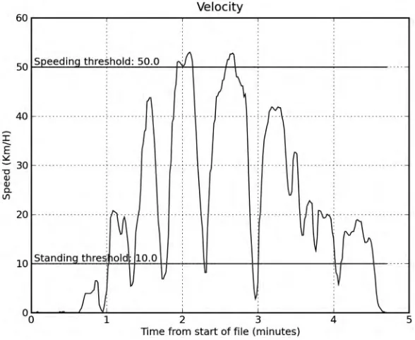
In the case of a CLCOR header, the number of satellites is the fourth entry. In case of a CLNI?

header, we have a bit more interesting information. The second field is the timestamp, the fourth field is the latitude, the sixth field is the longitude, and the eighth field is the velocity. Again, turn to the NMEA 0183 format for more details. Table 1-1 summarizes the fields and their values in a CLNI? line.

Table 1-1. CLNI? Information (Excerpt)

Field Name Index Format

Header 0 CLNI? (fixed)

Timestamp 1 hhmmss.ss

Latitude 3 DDMM.MMM

,ONGITUDE

$$$---Velocity 7 VVV.V

:::tW-.Y

W# CLNI?#(#-0,,11*,,#(#=#(#0010*-30,#(#J#(#,5/.1*,-0/#(#S#(#,,,*,#(#-.4*3#( #/,,1,4#(#,,-*-#(#A#(#=&.4#Y

In this output, the timestamp appears as #-0,,11*,,#. This follows the format hhmmss.ss where hh are two digits representing the hour (it will always consist of two digits—if the hour is one digit, say 7 in the morning, a 0 will be added before it), mm are two digits representing the minute (again, always two digits), and ss.ss are five characters (four digits plus the dot) representing seconds and fractions of seconds. (There’s also a North/South field as well as an East/West field. Here, for simplicity, we assume northern hemisphere, but you can easily change these values by reading the entire CLNI? structure.)

N

Note

In the ISO time format, we’ve used HHMMSS to denote hours minutes and seconds. Here we follow the convention in NMEA, which uses hhmmss.ss for hours, minutes, and seconds and sets DD and MM to angular degrees and minutes.

The timestamp string is a bit hard to work with, especially when plotting data. The first reason is that it’s a string, not a number. But even if you translated it to a number, the system does not lend itself nicely to plotting because there are 60 seconds in a minute, not a 100. So what we want to do is “linearize” the timestamp. To achieve this, we translate the timestamp as seconds elapsed since midnight, as follows: T = hh * 3600 + mm * 60 + ss.ss.

The second issue we have is that hh, mm, and ss.ss are strings, not numbers. Multiplying a string in Python does something completely different from what we want here. So we have to first convert the strings to numerical values, in our case, bhk]p, because of the decimal point in the string representing the seconds. This all folds nicely into the following:

:::nks9tW-.Y

W# CLNI?#(#-0,,11*,,#(#=#(#0010*-30,#(#J#(#,5/.1*,-0/#(#S#(#,,,*,#(#-.4*3#( #/,,1,4#(#,,-*-#(#A#(#=&.4#Y

:::bhk]p$nksW-YW,6.Y%&/2,,'bhk]p$nksW-YW.60Y%&2,'bhk]p$nksW-YW062Y% 1,001*,

The operator WY denotes the index, so nksW-Y is the second field of nks (counting starts at zero) which is a string. The first two characters of a string are denoted by W,6.Y; this is known asstring slicing. So to access the first two characters of the first field, we write nksW-YW,6.Y. Upcoming chapters will include more about strings and methods of slicing them.

Next we tackle latitude and longitude. We face the same issue as with the timestamp, only here we deal with degrees. Latitude follows the format DDMM.MMM where DD stands for degrees and MM.MMM stands for minutes. We decide to use degrees this time. To translate the latitude into decimal degrees, we need to divide the minutes by 60:

:::nks9tW-.Y

W# CLNI?#(#-0,,11*,,#(#=#(#0010*-30,#(#J#(#,5/.1*,-0/#(#S#(#,,,*,#(#-.4*3#( #/,,1,4#(#,,-*-#(#A#(#=&.4#Y

&ORLATITUDEINFORMATIONWErequire the fourth field, hence nksW/Y. This example also introduces another notation, W.6Y, which means the slice of the string from the third character until the end. Also notice that the code uses 2,*, and not 2,. When dividing by 60, it’s implied that you want an integer division; dividing by 60.0 means you want a floating-point division, which is to say you care about the information past the decimal point. However, seeing as we already specified that we want the information as a floating-point number as indicated by the

bhk]p$% conversion, the result will be a floating point regardless. Still, it’s good practice to let Python know what kind of division you really want.

Here are some examples to further illustrate the point:

:::-,,+2,

-:::-,,+2,*, -*2222222222222223 :::bhk]p$-,,%+2, -*2222222222222223

Longitude information is similar to latitude with a minor difference: longitude degrees are three characters instead of two (up to 180 degrees, not just up to 90 degrees) so the indices to the strings are different.

Listing 1-6 presents the entire function to process GPS data.

Listing 1-6. Functionlnk_aoo[clo[`]p]$% bnkiluh]^eilknp&

_kjop]jp`abejepekjo JIE9-41.*,

`ablnk_aoo[clo[`]p]$`]p]%6

Lnk_aooaoCLO`]p](JIA=,-4/bkni]p*

Napqnjo]pqlhakb]nn]uo6h]pepq`a(hkjcepq`a(rahk_epuWgi+dY( peiaWoa_Y]j`jqi^ankbo]pahhepao*

Oaa]hok6dppl6++sss*cloejbkni]pekj*knc+`]ha+jia]*dpi*

h]pepq`a9WY hkjcepq`a9WY rahk_epu9WY p[oa_kj`o9WY jqi[o]po9WY

bknnksej`]p]6

ebnksW,Y99# CLCOR#6

jqi[o]po*]llaj`$bhk]p$nksW/Y%% ahebnksW,Y99# CLNI?#6

bhk]p$nksW/YW.6Y%+2,*,%

hkjcepq`a*]llaj`$$bhk]p$nksW1YW,6/Y%'X bhk]p$nksW1YW/6Y%+2,*,%%

rahk_epu*]llaj`$bhk]p$nksW3Y%&JIE+-,,,*,%

napqnj$]nn]u$h]pepq`a%(]nn]u$hkjcepq`a%(X

]nn]u$rahk_epu%(]nn]u$p[oa_kj`o%(]nn]u$jqi[o]po%%

Some notes about the lnk_aoo[clo[`]p]$% function:

sJIE is defined as -41.*,, which is one nautical mile in meters and also one minute on the equator. The reason the constant JIE is not defined in the function is that we’d like to use it outside the function as well.

s 7EINITIALIZETHERETURNVALUESh]pepq`a,hkjcepq`a,rahk_epu,p[oa_kj`o, and jqi[o]po

by setting them to an empty list: WY. Initializing the lists creates them and allows us to use the ]llaj`$% method, which adds values to the lists.

s 4HEeb and aheb statements are self-explanatory: eb is a conditional clause, and aheb is equivalent to saying “else, if.” That is, if the first condition didn’t succeed, but the next condition succeeds, execute the following block.

s 4HESYMBOLX that appears on the several calculations and on the napqnj line indicates that the operation continues on the next line.

s ,ASTLYTHERETURNVALUEISa tuple of arrays. A tuple is an immutable sequence, mean-ing you cannot change it. So tuple means an unchangeable sequence of items (as opposed to a list, which is a mutable sequence). The reason we return a tuple and not a two-dimensional array, for example, is that we might have different lengths of lists to return: the length of the number of satellites list may be different from the length of the longitude list, since they originated from different header stamps.

Here’s how you call lnk_aoo[clo[`]p]$%:

:::u9na]`[_or[beha$#**+`]p]XXCLO).,,4),1)/,),5),,)1,*_or#% :::$h]p(hkjc(r(p(o]po%9lnk_aoo[clo[`]p]$u%

The second line introduces sequence unpacking, which allows multiple assignments. Armed with all these functions, we’re ready to plot some data!

Data Visualization

Our next step is to visualize the data. We’ll be relying on the matplotlib package heavily. We’ve already imported matplotlib with the command bnkiluh]^eilknp&, so there’s no additional importing needed at the moment. It’s time to read the data and plot the course.

Listing 1-7. “Quick-and-Dirty” Spherical to Cartesian Transformation

t9hkjcepq`a&JIE&2,*,&_ko$h]pepq`a% u9h]pepq`a&JIE&2,*,

To justify this to yourself, consider the following reasoning: As you go up to the North Pole, the circumference at the location you’re at gets smaller and smaller, until at the North Pole it’s zero. So at latitude 0º, the equator, each degree (longitude) means more distance trav-ELEDTHANATLATITUDEŽ4HATSWHYt is a function of the longitude value itself but also of the latitude: the greater the latitude, the smaller a longitude change is in terms of distance. On the other hand, u, which is north to south, is not dependent on longitude.

The next thing to understand is that the earth is a sphere, and whenever we plot an x-y map, we’re only really plotting a projection of that sphere on a plane of our choosing, hence we denote it by (px,py), where p stands for “projection.” We’ll take the southeastern-most point as the start of the GPS data projection: (px,py) = (0,0). This translates into the code shown in Listing 1-8.

Listing 1-8. Projecting the Traveled Course to Cartesian Coordinates

lu9$h]p)iej$h]pepq`a%%&JIE&2,*,

lt9$hkjc)iej$hkjcepq`a%%&JIE&2,*,&[email protected]&h]pepq`a%

Some things to note:

s 6ARIABLESlu and ltare arrays of floating-point values. We now operate on entire arrays seamlessly. This is part of the NumPy package.

[email protected] is a constant equal to ›/180, converting degrees to radians.

s 4OSETTHEYAXISATTHEMINIMUMLATITUDEANDTHEXAXISATTHEMINIMUMLONGITUDEWE subtract the minimum latitude and minimum longitude values from latitude and lon-gitude values, respectively.

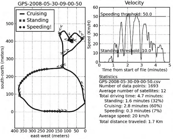
GPS Location Plot

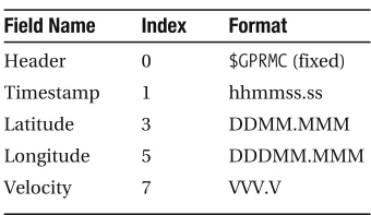
Now the moment we’ve been waiting for, plotting GPS data. To be able to follow along and plot data, be sure to define the functions na]`[_or[beha$% and lnk_aoo[clo[`]p]$% as previ-ously detailed and set the file name variable to point to your GPS data file. I’ve suppressed matplotlib responses so that the code is cleaner to follow.

:::behaj]ia9#CLO).,,4),1)/,),5),,)1,*_or# :::u9na]`[_or[beha$#**+`]p]+#'behaj]ia% :::$h]p(hkjc(r(p(o]po%9lnk_aoo[clo[`]p]$u% :::lt9$hkjc)iej$hkjc%%&JIE&2,*,&[email protected]&h]p% :::lu9$h]p)iej$h]p%%&JIE&2,*,

:::becqna$%

:::c_]$%*]tao*ejranp[t]teo$%

:::lhkp$lt(lu(#^#(h]^ah9#?nqeoejc#(hejase`pd9/% :::pepha$behaj]iaW6)0Y%

:::uh]^ah$#okqpd)jknpd$iapano%#% :::cne`$%

:::]teo$#amq]h#% :::odks$%

&IGURESHOWSTHERESULTWHICHISRATHERPLEASING

Figure 1-1. GPS data

We’ve used a substantial number of new functions, all part of the matplotlib package:

lhkp$%,cne`$%,th]^ah$%,hacaj`$%, and more. Most of them are self-explanatory:

sth]^ah$opnejc[r]hqa% and uh]^ah$opnejc[r]hqa% will print a label on the x- and y-axis, respectively.pepha$opnejc[r]hqa% is used to print a caption above the graph. The string value in the title is the file name up to the end minus four characters (so as to not dis-play “.csv”). This is done using string slicing with a negative value, which means “from the end.”

shacaj`$% prints the labels associated with the graph in a legend box. hacaj`$% is highly configurable (see dahl$hacaj`% for details). The example plots the legend at the top-left corner.

scne`$% plots the grid lines. You can control the behavior of the grid quite extensively.

slhkp$% requires additional explanation as it is the most versatile. The command

s 4HEFUNCTION]teo$% controls the behavior of the graph axis. Normally, I don’t call the

]teo$% function because lhkp$% does a decent job at selecting the right values. How-ever, in this case, it’s important to visualize the data properly, and that means to have both x- and y-axes with equal increments so the graph is true to the path depicted. This is achieved by calling ]teo$#amq]h#%. There are other values to control axis behavior as described bydahl$]teo%.

s ,ASTLYc_]$%*]tao*ejranp[t]teo$% is a rather exotic addition. It stems from the way we like to view maps and directions. In longitude, increasing values are displayed from right to left. However, in mathematical graphs, increasing values are typically displayed from left to right. This function call instructs the x-axis to be incrementing from right to left, just like maps.

s 7HENYOUREDONEPREPARINGthe graph, calling the odks$% function displays the output.

Matplotlib, which includes the preceding functions, is a comprehensive plotting package and will be explored in Chapter 6.

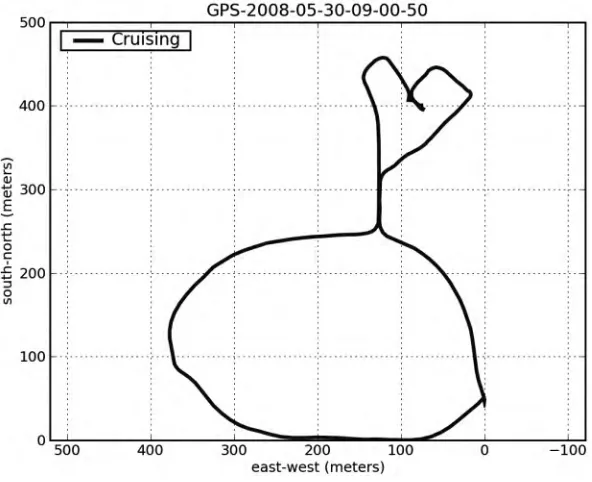
Annotating the Graph

We’d like to add some more information to the GPS graph: we’d like to know where we’ve STOPPEDANDWHEREWEWERESPEEDING&ORTHISWEUSETHEFUNCTIONbej`$%, which is part of the PyLab package. bej`$% returns an array of indices that satisfy the condition, in our case:

:::OP=J@EJC[GID9-,*, :::OLAA@EJC[GID91,*,

:::Eop]j`9bej`$r8OP=J@EJC[GID% :::Eolaa`9bej`$r:OLAA@EJC[GID%

:::E_nqeoa9bej`$$r:9OP=J@EJC[GID%"$r89OLAA@EJC[GID%%

We also calculate when we’re cruising (i.e., not speeding nor standing) for future process-ing.

To annotate the graph with these points, we add another plot on top of our current plot, only this time we change the color of the plot, and we use symbols instead of a solid blue line. The combination #oc# indicates a green square symbol (g for green, s for square); the combi-nation#kn# indicates a red circle (r for red, o for circle). I suggest you use different symbols for standing and speeding, not just colors, because the graph might be printed on a monochrome printer. The function lhkp$% supports an assortment of symbols and colors; consult with the interactive help for details. The values we plot are only those returned by thebej`$% function.

:::lhkp$ltWEop]j`Y(luWEop]j`Y(#oc#(h]^ah9#Op]j`ejc#% :::lhkp$ltWEolaa`Y(luWEolaa`Y(#kn#(h]^ah9#Olaa`ejc#% :::hacaj`$hk_9#qllanhabp#%

Figure 1-2. GPS data with additional speed information

We’d also like to know the direction the car is going. To implement this, we’ll use the

patp$% function, which allows the writing of a string to an arbitrary location in the graph. So to add the text “Hi” at location (10, 10), issue the command patp$-,(-,(#De#%. One of the nice features of the patp$% function is that you can rotate the text at an arbitrary angle. So to PLOTh(IvATLOCATION ATDEGREESYOUISSUEpatp$-,(-,(#De#(nkp]pekj901%. Our implementation of heading information involves rotating the text “>>>” at the angle the car is heading. We’ll only do this ten times so as not to clutter the graph with “>” symbols. Calculat-ing the direction the car is headCalculat-ing at a given point, e, is shown in Listing 1-9.

Listing 1-9. Calculating the Heading

`t9ltWe'-Y)ltWeY `u9luWe'-Y)luWeY da]`ejc9]n_p]j$`u+`t%

Instead of actually using the function ]n_p]j$`u+`t%, we’ll use the function ]n_p]j.$`u( `t%. The benefits of using ]n_p]j.$% over ]n_p]j$% are twofold: 1) there’s no division that might cause a divide-by-zero exception in case `t is zero, and 2) ]n_p]j.$% preserves the angle from –180 degrees to 180 degrees, whereas ]n_p]j$% produces values between 0 degrees and 180 degrees only. The following code adds the direction symbols:

:::bkneejn]jca$,(haj$r%(haj$r%+-,)-%6 ***patp$ltWeY(luWeY(:::(X

&IGURESHOWSTHEresulting graph.

Figure 1-3. GPS graph with heading

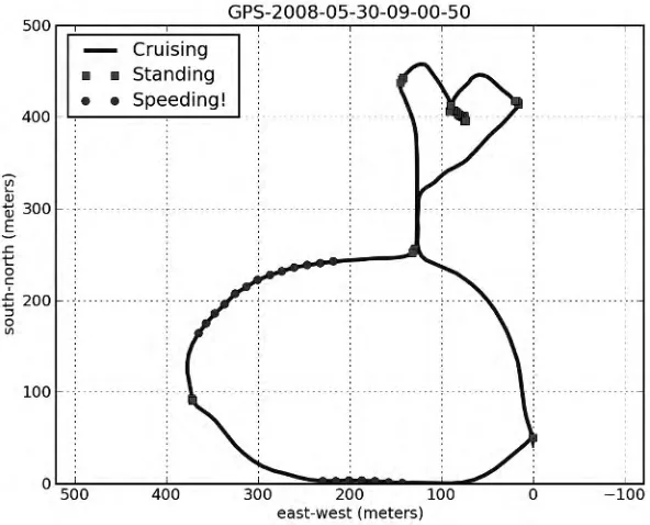
Velocity Plot

We now turn to plotting a graph of the speed. This is a lot simpler:

:::becqna$%

:::p9$p)pW,Y%+2,*, :::lhkp$p(r(#g#%

:::lhkp$WpW,Y(pW)-YY(WOP=J@EJC[GID(OP=J@EJC[GIDY(#)c#% :::patp$pW,Y(OP=J@EJC[GID(X

***Op]j`ejcpdnaodkh`6'opn$OP=J@EJC[GID%%

:::lhkp$WpW,Y(pW)-YY(WOLAA@EJC[GID(OLAA@EJC[GIDY(#)n#% :::patp$pW,Y(OLAA@EJC[GID(X

***Olaa`ejcpdnaodkh`6'opn$OLAA@EJC[GID%% :::cne`$%

:::pepha$#Rahk_epu#%

:::th]^ah$#Peiabnkiop]npkbbeha$iejqpao%#% :::uh]^ah$#Olaa`$Gi+D%#%

graphs require annotation, so we choose to add two lines describing the thresholds for stand-ing and speedstand-ing as well as text describstand-ing those thresholds. To generate the text, we combine the text “Standing threshold” with the threshold value (after casting it to a string) and use the '

OPERATORTOCONCATENATESTRINGS,ASTOFCOURSEARETHETITLEXANDYLABELSANDGRID&IGURE shows the final result.

Figure 1-4. Velocity over time

Subplots

We’d also like to display some statistics. But before we do that, it would be preferable to combine all these plots (GPS, velocity, and statistics) into one figure. To do this, we use the

oq^lhkp$% function. oq^lhkp$% is a matplotlib function that divides the plot into several smaller SECTIONSCALLEDSUBPLOTSANDSELECTSTHESUBPLOTTOWORKWITH&OREXAMPLEoq^lhkp$-(.(-%

informs subsequent plotting commands that the area to work on is 1 by 2 subplots and the currently selected subplot is 1, so that’s the left side of the plot area. oq^lhkp$.(.(.% will choose the top-right subplot; oq^lhkp$.(.(0% will choose the lower-right subplot. A selec-tion I found most readable in this scenario is to have the GPS data take half of the plot area, the velocity graph a quarter, and the statistics another quarter.

Text

To print the text on the canvas, we again use the patp$% function, in a bkn loop, iterating over every string of the op]po list.

:::bknej`at(op]p[hejaejajqian]pa$naranoa`$op]po%%6 ***patp$,(ej`at(op]p[heja(r]9#^kppki#%

***

:::lhkp$Wej`at)*.(ej`at)*.Y% :::]teo$W,(-()-(haj$op]po%Y%

We’ve introduced two new functions. One is naranoa`$%, which yields the elements of

op]po, in reversed order. The second is ajqian]pa$%, which returns not just each row in the

op]po array but also the index to each row. So when variable op]p[heja is assigned the value

#=ran]caolaa`***#, the variable ej`at is assigned the value 4, which indicates the ninth row inop]po. The reason we want to know the index is that we use it as location on the y-axis. Lastly, the vertical alignment of the text is selected as bottom as suggested by the parameter

r]9#^kppki# (r] is short for vertical alignment).

Tying It All Together

&INALLY,ISTINGSHOWSTHEcombined code to analyze and plot all GPS files in directory `]p].

Listing 1-10. Scriptclo*lu bnkiluh]^eilknp& eilknp_or(ko

_kjop]jp`abejepekjo OP=J@EJC[GID9-,*, OLAA@EJC[GID91,*, JIE9-41.*, @.N9le+-4,*,

`abna]`[_or[beha$behaj]ia%6

Na]`o]?ORbeha]j`napqnjoep]o]heopkbnkso*

`]p]9WY

bknnksej_or*na]`an$klaj$behaj]ia%%6 `]p]*]llaj`$nks%

napqnj`]p]

`ablnk_aoo[clo[`]p]$`]p]%6

Lnk_aooaoCLO`]p](JIA=,-4/bkni]p*

Napqnjo]pqlhakb]nn]uo6h]pepq`a(hkjcepq`a(rahk_epuWgi+dY( peiaWoa_Y]j`jqi^ankbo]pahhepao*

h]pepq`a9WY hkjcepq`a9WY rahk_epu9WY p[oa_kj`o9WY jqi[o]po9WY

bknnksej`]p]6

ebnksW,Y99# CLCOR#6

jqi[o]po*]llaj`$bhk]p$nksW/Y%% ahebnksW,Y99# CLNI?#6

p[oa_kj`o*]llaj`$bhk]p$nksW-YW,6.Y%&/2,,'X bhk]p$nksW-YW.60Y%&2,'bhk]p$nksW-YW062Y%% h]pepq`a*]llaj`$bhk]p$nksW/YW,6.Y%'X bhk]p$nksW