Volume 40, Number 3 (May 1987)

(1)

Vol. 40, No. 3, May 1987

ARTICLES

Range Improvement

194 Leafy Spurge Control and Herbicide Residue from Annual Piclornm and 2,4-D Application by Rodney G. Lym and Calvin G. Messersmith

199 Integration of Cattle Production and Marketing Strategies with Improved Pastures and Native Range by D.E. Ethridge, J.D. Nance, and B.E. Dahl

Plan Is

203 Leaf Water Potential Trends in Three Grasses Native to Semiarid Argentina by Roberto A. Distel and Osvaldo A. Fernandez

207 Caryopsis Weight and Planting Depth of Blue Grama I. Morphology, Emergence, and Seedling Growth by C.J. Carren, A.M. Wilson, R.L. Cuany, and G.L. Thor 212 Caryopsis Weight and Planting Depth of Blue Grama II. Emergence in Marginal

Soil Moisture, by C.J. Carren, A.M. Wilson, and R.L. Cuany Grazirw

216 1% vs. 42-Paddock Rotational Grazing: Aboveground Biomass Dynamics, Forage Production, and Harvest Efficiency by R.K. Heitschmidt, S.L. Dowhower, and J.W. Walker

224

228

232

237

The Influence of Grazing Pressure on Rooting Dynamics of Caucasian Bluestem by Tony Svejcar and Scott Christiansen

Defoliation of Intermediate Wheatgrass under Seasonal and Short-duration Graz- ing by Frederick B. Pierson and David L. Scarnecchia

Persistence of a Loliumperenne-Trifolium subterraneum Pasture under Differing Defoliation Treatments by Iraj Motazedian and Steven H. Sharrow

Herbage Standing Crop around Eastern Redcedar Trees by D.M. Engle, J.F. Stritzke, and P.L. Claypool

Hydrology

240 Infiltration Rates and Sediment Production as Influenced by Grazing Systems in the Texas Rolling Plains by J.J. Pluhar, R.W. Knight, and R.K. Heitschmidt Digestibility

244 Crude Terpenoid Influence on In Vitro Digestibility of Sagebrush by Karl D. Striby, Carl L. Wambolt, Rick G. Kelsey, and Kris M. Havstad

Career

249 Career Development of Range Conservationists in Their First Three Years with the Forest Service by James J. Kennedy

Range Research

254 Nondestructive Estimation of Shortgrass Aerial Biomass by Samuel C. William- son, James K. Detling, Jerrold L. Dodd, and Melvin 1. Dyer

256 An Automated Range-animal Data Acquisition System by D.C. Adams, P.O. Currie, B.W. Knapp, T. Mauney, and D. Richardson

259 Plot Numbers Required to Determine Infiltration Rates and Sediment Production on Rangelands in South Central New Mexico by M. Karl Wood

Soil Bacteria and Fungi

264 Distribution and Symbiotic Effectiveness of Rhizobium me&M in Rangeland Soils of the Intermountain West by W.L. Lowther, D.A. Johnson, and M.D. Rumbaugh

268 Populations of Rhizobium meliloti in Areas with Rangeland Alfalfa by W.L. Lowther, M.D. Rumbaugh, and D.A. Johnson

(2)

Published bimonthly-January, March, May, July, September, November

INDIVIDUAL SUBSCRIPTION is by membership in INSTITUTIONAL SUBSCRIPTIONS on a calendar year basis are $56.00 for the United States postpaid and the Society for Range Management.

LIBRARY or other $66.00 for other countries, post- paid. Payment from outside the United States should be remitted in US dollars by international money order or draft on a New York bank.

BUSINESS CORRESPONDENCE, concerning sub- scriptions, advertising, reprints, back issues, and related matters, should be addressed to the Manag- ing Editor, 1639 York Street, Denver, Colo. 60206. EDITORIALCORRESPONDENCE, concerning manu- scriptsorothereditorial matters, should beaddressed to the Editor, 1639 York Street 80206.

INSTRUCTIONS FOR AUTHORS appear on the inside back cover of each issue. A Style Manual is also available from the Society for Range Manage- ment at the above address@$1.25 for single copies; $1 .W each for 2 or more.

THE JOURNAL OF RANGE MANAGEMENT (ISSN 0022~409X) is published six times yearly for $56.00 per year by the Society for Range Management, 1639 York Street, Denver, Colo. 60206. SECOND CLASS POSTAGE paid at Denver, Colo. POSTMASTER: Return.entire journal wlth address change--RETURN POSTAGE GUARANTEED-to Society for Range Management, 1639 York Street, Denver, Colo. 60206.

The Journal of Range Management serves as a forum for the presentation and discussion of facts, ideas, and philosophies pertaining to the study, management, and use of range- lands and their several resources. Accord- ingly, all material published herein is signed and reflects the individual viewsof the authors and is not necessarily an official position of the Society. Manuscripts from any source- nonmembers as well as members-are wel- come and will be given every consideration by the editors. Submissions need not be of a technical nature, but should be germane to the broad field of range management. Editor- ial comment by an individual is also welcome and subject to acceptance by fhe editor, will be published as a “Viewpoint.”

Managlng Edltor PETER V. JACKSON Ill

1639 York Street Denver, Colorado 60208 Editor

PATRICIA G. SMITH

Society for Range Management 1639 York Street

Denver, Colorado 60206 Book Review Editor GRANT A. HARRIS

Forestry and Range Management Washington State University Pullman. Washington 991646410

Knapweed

277 Nutrient Composition of Spotted Knapweed

(Centaurea maculosa) by

Rick G. Kelsey and Robert D. Mihalovich

TECHNICAL NOTES

282

284

285

A Temporary Esophageal Cammla that Prevents Fistula Contraction during Extrusa Collections by K.C. Olson and J.C. Malechek

The Use of a Portable Computer for Real-time Recording of Observations of Grazing Behavior in the Field by Montague W. Demment and Gregory B. Greenwood

Effect of Hydroelutriation on Nonstructural Carbohydrates in Fibrous Roots by Tony Svejcar and Scott Christiansen

BOOK REVIEWS

287 Wildflowers of the Canadian Rockies. by George W. Scatter and Halle Flygare; Arid and Semiarid Lands; Sustainable Use and Management in Developing Coun- tries by R. Dennis Child, Harold F. Heady, Wayne C. Hickey, Ronald A. Peterson, and Rex D. Pieper; Introduction to Wildlife Management by James H. Shaw; North American Range Plants by J. Stubbendieck, S.L. Hatch, and Kathie Hirsch; Beef, Brush and Bobwhites: Quail Management in Cattle Country by Fred S. Guthery; Conservation Biology: the Science of Scarcity and Diversity edited by Michael E. Some: and The Practice of Silviculture. 8th Edition, by David M. Smith.

ASSOCIATE EDITORS G. FRED GIFFORD

Dept. of Range Wildlife, and Forestry University of Nevada

Reno. Nev. 69506 THOMAS A. HANLEV

Forestry Sciences Lab. Box 969

Juneau, Alaska 99602 RICHARD H. HART

USDA-ARS 6406 Hildreth Rd. Cheyenne, Wyoming 62009 N. THOMPSON HOBBS

Colorado Div. of Wildlife 317 W. Prospect

Fort Collins, Colorado 60526 W.K. LAUENROTH

Department of Range Science Colorado State University Fort Collins, Colorado 60523

BRUCE ROUNDV 325 Biological Sciences East Building, Univ. Arizona Tucson, AZ 65721 NEIL E. WEST

Range Science Department Utah State University UMC 52 Logan, Utah 64322

LARRY M. WHITE USDA ARS

S. Plains Range Research Station 2000 16th St.

Woodward, Oklahoma 73801 RICHARDS. WHITE

USDA-ARS Route 1, Box 2021 Miles City, Montana 59301 STEVE WHISENANT

401 Widtsoe Building Brigham Young Univ. Provo, Utah 64602 HOWARD MORTON

2ooO E. Allen Road Tucson, Arizona 65719

JAMES YOUNG USDA ARS

(3)

(4)

Leafy Spurge Control and Herbicide Residue From Annual

Picloram and 2,4-D Application

RODNEY G. LYM AND CALVIN G. MESSERSMITH

Abstract

Annual application of picloram (4amino-3,5,6-trichloro-2-py- ridinecarboxylic acid) and picloram plus 2,4-D [(2,4-dichloro- phenoxy)acetic acid] and biannual application of 2,4-D for 5 con- secutive years was evaluated for leafy spurge (Euphorbia esula L.) control. The picloram treatments were evaluated for soil residue. The experiment was located at 2 sites in eastern North Dakota and 1 site in western North Dakota on various soil types. Picloram at 0.28,0.42, and 0.56 kg/ha provided 48,75, and 90% leafy spurge control after 4 annual treatments, respectively. Control increased to 85 and 91% when 2,4-D at 1.1 kg/ha was added to the amural treatment of picloram at 0.28 and 0.42 kg/ha, respectively. How- ever, 2,4-D with picloram at 0.56 kg/ha did not increase leafy spurge control compared to picloram alone.

Picloram did not accumulate in the upper 15 cm of the soil profile and generally was not detected above the 2 ppbw level 12 months following each annual application. Greater picloram residue was found deeper in sandy than clay soil and in soil with high compared to low organic matter. Picloram at 500 and 250 ppbw was required to reduce leafy spurge seedling emergence and subsequent survival by 50$& respectively. However, picloram at 125 ppbw reduced leafy spurge regrowth from root segments of 4 lengths to near zero. Picloram at 8 to 32 ppbw stimulated leafy spurge seedling emergence compared to the control. Annual appli- cation of picloram at low rates gradually controlled leafy spurge, but picloram soil residues were not high enough to control subse- quent seed germination and shoot regrowth from roots.

Key words: herbicide interaction, Euphorbia es& L., HPLC Picloram (4amino-3,5,6-trichloro-2-pyridinecarboxylic acid) is the most effective herbicide for control of leafy spurge (Euphorbia esulu L.) (Lym and Messersmith 1985a). Picloram at 2.2 kg/ ha has given 80% leafy spurge control 27 months after application in North Dakota and for 36 to 39 months in Wyoming (Alley et al. 1983). The cost of picloram at 2.2 kg/ ha is often 5% or more of the total land value and 8 to 10 times higher than the cash rent value of pasture and rangeland (Johnson 1984). Thus, it often is not eco- nomical to control leafy spurge with high rates of picloram on large infestations in pasture and rangeland.

24-D [(2,4dichlorophenoxy)acetic acid] dimethylamine at 1.1 kg/ ha enhanced leafy spurge control when applied with picloram at 0.6 kg/ ha or less (Lym and Messersmith 1985a). Annual treatment of picloram at 0.3 to 0.6 kg/ ha with 2,4-D at 0.3 to 1.1 kg/ ha gradually improved leafy spurge control to 80% or better after 3 years. This combination treatment also increased forage production up to 71% and reduced leafy spurge yield by 96% after 3 annual applications in North Dakota (Lym and Messersmith 1985b).

Annual application of picloram could become an environmental hazard because of long persistence, relatively high water solubility and leaching potential, and high phytotoxicity. However, residue from picloram applied at 0.56 kg/ha or less generally does not persist in the environment. Herr et al. (1966) found that the highest picloram concentration in heavy to medium textured soil following annual application was near the surface but picloram residue was much deeper in light textured soil. Picloram dissipated faster at

Authors are assistant professor and professor of agronomy, North Dakota State University, Fargo, N.D. 58105.

Published with the approval of the Director, Agricultural Experiment Station, North Dakota State University as Journal Article No. 1480.

Manuscript accepted 24 September 1986.

low than high application rates on all 3 soil types. Picloram applied on rangeland generally has dissipated rapidly with the highest concentration remaining in the top 15 cm of the soil profile (Scifres et al. 1977). Picloram applied at 0.28 kg/ ha or less often dissipated within 60 days (Bauer et al. 1972; Scifres et al. 1971a, 1971b). Picloram at 2.2 kg/ ha applied 5 times in 2 years did not accumulate in the vegetation, soil profile, or well water on the prairie ecosys- tems of central Texas (Bovey et al. 1974, 1975).

The purpose of this study was to evaluate various annual picloram and 2,4-D treatments for leafy spurge control and determine picloram soil residue and effect on seedling emergence and growth in 3 areas of North Dakota following a 5-year annual treatment program.

Materials and Methods

An experiment to evaluate leafy spurge control from annual applications of picloram and picloram plus 2,4-D and biannual application of 2,4-D alone was established at 3 sites in North Dakota. The sites included a bluegrass (Pea spp.) pasture near Sheldon, a mixed grass prairie on a federal game management area near Valley City, both in eastern North Dakota, and a mixed grass pasture near Dickinson in western North Dakota. Soil properties and annual precipitation received during the study at each site are listed in Table 1. All sites had at least an 80% ground cover of leafy spurge with few other forbs present.

Herbicides were applied using a tractor mounted sprayer deliver- ing 75 L/ha water at 240 kPa. The experiment was begun on 25 August 1981 at Dickinson, 1 September 1981 at Sheldon, and 11 June 1982 at Valley City. All treatments were applied annually except 2,4-D alone which was applied biannually (twice per year). Picloram treatments were applied in late August 1981 and in June 1982 through 1985. The 2,4-D biannual treatments were applied in June and August of each year. Thus, the Dickinson and Sheldon sites were sprayed with picloram and picloram plus 2,4-D treatments 5 times, and 24-D alone 8 times, while the Valley City site received 4 and 7 treatments, respectively. Herbicides were applied when leafy spurge was flowering in June or had resumed fall regrowth following a summer dormancy period in August. The plots were 3.1 by 9.1 m and each treatment was replicated 4 times in a randomized complete block at all sites. Evaluations were based on visual percent stand reduction as compared to the control.

Soil samples for picloram residue analysis were taken twice each year except 1985 at all locations. The first yearly sample was collected prior to herbicide application in June and the second in late August or early September from the untreated control and picloram-alone treated plots. Three subsamples 15-cm deep were collected per plot and combined for each sampling date from 1982 through 1984. Four subsamples 120-cm deep were collected per plot in September 1985 and divided into 5 segments consisting of 0 to 15, 15 to 30, 30 to 60,60 to 90, and 90 to 120 cm depths and combined.

(5)

Table 1. Physical and chemical characteristics of soils and ammal precipitation at the various study sites in North Dakota.

Precipitation

1981 1982 1983 1984 1985

Cation Trt. Trt. Trt. Tit. Trt.

ex- to’b t0.b toab t0.b to-b

Organic change samp- samp- samp- samp- samp-

Location Soil type Sand Silt Clay matter pH capacity ling Annual ling Annual ling Annual ling Annual ling Annual

---+%)_-- (mesi -_--_

Sheldon Hamar- 100 g)

___---(cm)__---_

Ulehfine 78 13 9 2.1 7.7 12.8 27.1 58.3 15.7 51.6 19.0 46.3 10.4 53.5 15.3 38.2

sandy loam (166) (76) (65) (95) (76)

Valley Barnes 43 41 16 9.4 6.7 37.7 45.0 45.4 22.5 36.0 11.0 38.8 15.3 42.0

City stony loam (73) (92) (78)

Dickinson Felor loam 17 56 27 3.6 6.6 20.0 47.0 40.0 13.3 60.1 14.5 39.5 20.8 45.2 13.0 43.4

(167) (86) (72) (90) (105)

‘Number in ( ) are the number of days from treatment to sampling each year. ?reatment applied fall 1981 and in June each year thereafter.

contained enough picloram to give the required concentration were added to each 500-g soil sample, air dried for 18 h, and thoroughly mixed. The samples for both the standard curve and field samples were placed in ll- by 1 I- by 5-cm plastic pots, watered to 80% field capacity, and allowed to equilibrate for 24 h. Eight sunflower seeds were placed on the soil surface and covered with 2 cm of Styrofoam beads. The pots were arranged in a com- pletely random design in a greenhouse at 24O C, and natural light was sup_gleTented by metal halide lights with an intensity of 450 PE l m l s ‘for a 16-h photoperiod. The pots were rerandomized weekly. Sunflowers were harvested after 30 days. The topgrowth was oven dried at 60” C. A linear standard curve was calculated using regression analysis (Stat. Anal. Syst. 1982), and the mean sunflower dry weights for field samples were compared to those from known concentrations to estimate picloram concentration.

Picloram concentration from the samples collected in 1985 was determined by high pressure liquid chromatography (HPLC). Soil samples were dried and mixed as described earlier. Replicate 40-g soil samples were placed in 250-ml flasks, and then 80 ml of acetonitrile/water/ammonium hydroxide (70: 18:12, v/v/v) were added and shaken for 0.5 h. The soil samples were held at room

temperature for 18 h and then shaken a second time for 0.5 h (Smith and Milward 1983). The sample was vacuum filtered through 6 pm filter paper and the aqueous extract was evaporated to approximately 14 ml with a rotary evaporator at 40’ C. The sample was brought to 40 ml with 5% aqueous sodium carbonate (w/v) and centrifuged for 10 min at 10,000 rpm. The sample was filtered a second time through an 0.2 pm glass fiber syringe filter and then brought to 100 ml with the 5% sodium carbonate solution. The solution was transferred to a separatory funnel and extracted with 25 ml N-hexane. The inorganic fraction was discarded.

The aqueous phase containing picloram was acidified with 15 ml concentrated sulfuric acid. The sample was further clarified by adding 1.5 ml of saturated potassium permanganate and held at room temperature for 5 min, after which 5 M sodium bisulfite was added dropwise until the solution was colorless (Wells et al. 1984). The sample was extracted twice with 10 ml of methylene chloride and the eluate was evaporated to dryness on a rotary evaporator. The concentrated sample was redissolved in 3 ml of acetonitrile/- water (60:40, v/v) and a 10 PL injection of the eluate from this procedure was quantified by HPLC using a C-18 reverse-phase cartridge (0.45 i.d. by 25 cm). The solvent system consisted of:

Table 2. Leafy spurge control from five annual picloram or picloram plus 2,4-D treatmentsand eight biannual 2,4-D treatments at three locations in North Dakota.

Herbicide

Picloram Picloram Picloram 2,4-D biannual 2,4-D biannual 2,4-D biannual Picloram+2,4-D Picloram+2,4-D Picloram+Z,CD Picloram+2,4-D Picloram+Z,CD Picloram+2,4-D Picloram+Z,CD Picloram+2,4-D Picloramt2,CD

LSD (0.05)

Rate

(kg/ ha)

0.28 0.42 0.56 I.1 1.6 2.2 0.28+l.l 0.28+1.6 0.28t2.2 0.42t1.1 0.42tl.6 0.42t2.2 0.56+l.l 0.56+ I .6 0.56+2.2

Site and I985 evaluation date

Sheldon Dickinson Valley City’

June Aug June Aug June Aug I2

---@I control)-

I2 60 61 35 34 39 39

55 88 66 62 78 48 65

87 94 77 86 58 59 65

31 61 44 43 23 31 22

35 74 31 21 38 52 22

51 87 29 21 41 46 19

48 85 82 84 51 74 52

72 91 71 75 48 60 58

70 95 71 71 58 70 57

77 97 82 84 65 72 69

63 96 85 93 69 82 68

90 99 75 86 64 66 68

86 96 89 92 70 74 71

78 96 85 97 81 62 64

71 96 86 96 84 73 76

33 12 23 21 24 30 18

Mean

Months after treatment

24 36 48

_-_ ---

48 41 48

62 50 75

71 73 90

30 35 52

24 34 48

30 35 54

66 66 85

66 67 86

62 67 83

72 71 91

74 78 95

59 73 93

75 82 94

73 73 97

75 78 96

14 18 16

‘Experiment at Valley City received only4annual picloram or picloram plus 2,4-D treatments and 7 biannual 2,4-D treatments and data are not included in the 48 month mean.

(6)

eluent ‘A’, 1% acetic acid in water (v/v) and eluent ‘B’, 1% acetic acid in acetonitrile (v/v) using a linear gradient of 5 to 80% ‘B’in 25 min. The detector was a variable wavelength spectrophotometer operated at 254 nm. Retention time was approximately 9 min. Data were quantified by comparing peak areas against standards of known concentrations. Analysis of fortified samples indicated the least detectable limit was 0.5 ppb.

Leafy spurge seedling susceptibility to picloram was determined in a petri dish bioassay. Ten g soil samples were prepared as described in the bioassay experiment. Technical picloram at 2 to 1,000 ppbw was added to 4 replicate subsamples of untreated soil from each location. Ten leafy spurge seeds were planted per dish just below the soil surface and the dishes were placed in a growth chamber. The temperature was 30/ 20’ C (day/ night) for the first week and 25/20” C (day/ night) for the next 3 weeks with 80 to 90% relative humidity. A combination of fluorescent and incandescent bulbs provided 490 PE l me2 l s-r during the 12 h day. These are the optimum conditions for leafy spurge seed germination and seedling growth (Bakke 1936). Petri dishes were rotated weekly and plants were watered as needed. The percentage of emerged seed-

lings and seedling survival after 4 weeks was compared to the control.

Leafy spurge root segments 1, 5, 10, and 20 cm long of uniform diameter were obtained from 2-year-old greenhouse grown plants. One root segment was planted 1.5 cm deep per 4 cm diam by 20 cm long conical pot which contained 200 g of a soil-less medium of peat, perlite, and vermiculite. Technical picloram at 0 to 1,000 ppbw was added to the soil-less medium. The growth chamber temperature was 25/ 20” C (day/ night) with 50% relative humidity in a 16-h day. The number of emerged shoots was recorded 28 days after planting. A similar experiment was conducted using 200-g soil samples from the 3 field locations and IO-cm leafy spurge root segments. All growth chamber experimental designs were com- pletely random with 4 replications and repeated, except the field soil study which was repeated 3 times. Data for leafy spurge control, seed germination, and regrowth from root segments were analyzed using the general linear models procedure (Stat. Anal. Syst. 1982).

Table 3. Picloram concentration from various a~unl application rates for 4 years at three locations in North Dakota as determined by a sunflower bioassay iu 1982 through 1984 and HPLC in 1985.

Location Depth

Treatment rate

Sampling date

1982 1983 1984 1985

June _A% June _Aw June _Aw Sept

Sheldon (cm) O-15 15-30 30-60 60-90 90-120

Dickinson O-15

15-30

30-60

60-90

Valley City O-15

15-30 30-60 60-90 90-120 (kg/ ha) 0.28 0.42 0.56 0.28 0.42 0.56 0.28 0.42 0.56 0.28 0.42 0.56 0.28 0.42 0.56 0.28 0.42 0.56 0.28 0.42 0.56 0.28 0.42 0.56 0.28 0.42 0.56 0.28 0.42 0.56 0.28 0.42 0.56 0.28 0.42 0.56 0.28 0.42 0.56 0.28 0.42 0.56 c2

u

**

l

*

**

g

-a

**

*t

**

102 121 182 *** *** *** *** *** *** *** *** *** ***

2

11 *** *** *** *** *** *** ***

z

(2 *** *** *** *** *** *** *** *** *** *** *** c2

2 _**

**

2

IO ** ** ** ** ** ** ** ** l *

2 31 ** ** *+ ** ** ** ** ** ** ** ** ** I2 38 45 ** ** ** ** ** ** ** ** ** ** ** ** 10 13 83 ** ** ** ** ** l * ** ** ** 102 86 95 ** ** ** ** ** ** l * ** ** l * ** **

<2 55

c2 46

2

66 **

u **

15 **

** **

l * **

** ** ** ** ** +* ** ** =: 10 I3 <2 20

22 **

34 **

14 **

** ** ** ** ** ** ** ** ** ** ** **

22 64

65 126

55 I05

(7)

Results and Discussion

Picloram at 0.28,0.42, and 0.56 kg/ ha provided 48,75, and 90% leafy spurge control, respectively, after 5 annual applications when averaged across the Dickinson and Sheldon locations (Table 2). Control gradually improved over time with picloram at 0.42 and 0.56 kg/ ha, but not at the 0.28 kg/ ha application rate. Leafy spurge control from similar picloram applications averaged 39, 48, and 59%, respectively, following 4 annual treatments at Valley City.

Leafy spurge control was 5 1% following 8 biannual 2,4-D applications averaged over rate and location. Leafy spurge control gradually increased over time regardless of the 2,4-D application rate. However, Bybee and Messersmith (1976) reported that leafy spurge reestablished to the original density within 1 year after discontinuation of treatments that had been applied biannually for 4 to 5 years. Biannual 2,4-D treatment would be useful in areas where environmental conditions would prohibit picloram use but likely would only prevent leafy spurge seed production and spread with little change in area of the original infestation.

Leafy spurge control increased when 2,4-D was applied with picloram at 0.28 or 0.42 kg/ ha compared to picloram alone at similar application rates (Table 2). Control averaged 85 and 93% with picloram at 0.28 or 0.42 kg/ ha plus 2,4-D at 1.1 to 2.2 kg/ ha, respectively, compared to 48 and 75%, respectively, with similar picloram treatments applied alone. Picloram at 0.56 kg/ ha plus 2,4-D provided 96% leafy spurge control and was similar to picloram at 0.56 kg/ ha alone at 90% control. The benefit of applying 2,4-D with picloram for improved leafy spurge control decreased as the picloram rate increased. Leafy spurge control with picloram at 0.28 and 0.42 kg/ ha increased 37 and 18%, respectively, when averaged over all 2,4-D rates compared to similar picloram treatments applied alone. Leafy spurge control did not improve as the 2,4-D rate was increased from 1.1 to 2.2 kg/ ha in combination with picloram.

After 3 years of annual application of picloram at 0.56 kg/ha alone or at 0.28 and 0.42 kg/ ha with 2,4-D at 1.1 to 2.2 kg/ ha leafy spurge control was comparable to that from picloram applied once at 2.2 kg/ ha (Lym and Messersmith 1985b). Leafy spurge control with picloram at 2.2 kg/ha averaged 76 compared to 71% with picloram applied annually either at 0.56 kg/ ha alone or at 0.28 and 0.42 kg/ ha with 2,4-D at 1.1 to 2.2 kg/ ha. However, the combined 3-year annual treatment costs were 25,55 and 36% lower, respectively, compared to picloram applied once at 2.2 kg/ ha. Further- more, a retreatment following the picloram at 2.2 kg/ ha treatment would be necessary after the third year to maintain satisfactory leafy spurge control (Lym and Messersmith 1985a).

Picloram did not accumulate in the top 15 cm of the soil following annual application regardless of soil type or annual precipitation (Table 3). In general, picloram was not detected above 2 ppbw in the top I5 cm of the soil profile 12 months following application except at the Valley City site in 1984. The amount of picloram

detected in August of each year varied with the annual precipitation received from June to August; generally, more picloram remained in the upper 15 cm in drier than wet years (Tables 1 and 3). More picloram residue was retained in the upper 15 cm of soil at Valley City than at Dickinson and Sheldon probably because the Valley City soil contained more organic matter (Bauer et al. 1972; Herr et al. 1966; Phillips and Feltner 1972; and Scifres et al. 197la). The greater retention of picloram at Valley City also could explain the reduced leafy spurge control compared to the other 2 sites. Less picloram may have been available for root absorption especially at lower soil levels, thus limiting long-term leafy spurge root control.

Picloram was detected throughout the entire 120-cm soil profile sampled in 1985 at Sheldon and Valley City, but not at Dickinson (Table 3). In general, the picloram concentration in lower soil depths increased directly with the sand content of the soil. The soil at Sheldon has 71% sand and there was 14 ppbw picloram at 120 cm, while the soil at Dickinson has only 17% sand and no picloram was detected below 60 cm (Table 1). Picloram residues were not uniformly distributed throughout the soil profile. Picloram moves through soil in concentration pulses following high precipitation and is relatively immobile during drought periods (Neary et al. 1985). Thus, higher picloram residue at the 90 to 120 cm level than at 30 to 60 or 60 to 90 cm at Valley City and Sheldon, respectively, is probably due to concentration pulses. Generally, concentration pulse patterns at lower depths are of lower magnitude and delayed compared to upper soil levels.

Since picloram did not accumulate in the soil profile after 4 annual applications of 0.56 kg/ ha or less, this treatment program should not be considered an environmental hazard when herbicide label directions are followed. Previous studies have shown that residue in runoff water from picloram application of 0.56 kg/ ha or less was of little consequence especially 10 to 20 days after application (Bauer et al. 1972; Scifres et al. 1969, 197lb; Trichell et al. 1968). The possibility of accidental contamination of open wells or surface water still exists if the applicator is careless. Since picloram should not be applied in areas where the water table is within 3 m or less of the soil surface, introduction into underground water by leaching does not seem likely.

A picloram concentration of 500 and 250 ppbw was required to reduce leafy spurge seedling emergence and survival by at least 50%, respectively (Table 4). A picloram concentration of 8 to 32 ppbw tended to increase leafy spurge emergence compared to the control and did not affect seedling survival. Bowes and Thomas (1978) found that picloram concentrations up to 1,000 ppbw did not affect leafy spurge seed germination in the lab. Apparently, leafy spurge seed germination is not inhibited by picloram, but subsequent growth required for emergence is decreased at picloram concentrations of 500 ppbw or more.

Picloram at 125 ppbw was required to decrease seedling survival and 5% of the leafy spurge seedlings that emerged at 1,000 ppbw

Table 4. Leafy spurge seedling emergence and survival after 4 weeks in three North Dakota soil types and at various picloram concentrations.

Sheldon Picloram concentration Emergence Survival

(ppbw) ---

0 15 100

8 90 75

16 90 97

32 100 98

64 60 89

125 80 79

250 80 50

500 40 29

1000 40 6

LSD (0.05) 30 28

Soil location

Dickinson Valley City Mean

Emergence Survival Emergence Survival Emergence Survival

-_--I_-_ _-- --_---__

85 loo ---(%)- 60 100 13 100

100 100 100 100 97 100

100 96 100 96 97 100

90 95 70 95 87 96

75 89 70 86 68 88

80 72 65 52 75 68

60 56 70 34 70 47

40 19 50 9 43 19

40 4 50 4 43 5

27 16 31 32 19 17

(8)

picloram grew for at least 4 weeks in a growth chamber (Table 4). A higher mortality rate may be expected under field conditions where environmental conditions are less favorable for survival than in the growth chamber. However, less than 100 ppbw of picloram generally remained in the upper 15 cm of soil 3 months after application, so the herbicide residue probably would not limit the growth of leafy spurge seedlings. Indeed, the low concentration of picloram remaining in the soil 3 to 12 months after application may stimu- late leafy spurge seed germination.

Table 5. Leafy spurge shoot regrowth from root segments of four kngths exposed to various pkionm concentmtions for 28 days.

Picloram

concentration 1 cm

Original root length

5 cm 10 cm 20 cm

ppbw with

0 ---6----(% $roots sliits) 81

125 0 13 13 6

250 0 0 0 0

500 0 0 0 0

LSD (0.05) = 17

Lower picloram concentrations were required to control leafy spurge regrowth from roots than from seeds (Tables 4 and 5). More leafy spurge shoots were produced from 20 cm long root segments than shorter segments, but 5 and 10 cm long segments provided a similar number of new shoots when grown in a soil-less plant mixture. Regrowth was reduced when picloram at 125 ppbw was added to the soil-less medium, and no regrowth occurred at higher picloram concentrations.

Leafy spurge shoot regrowth increased as root segment length increased, but segment length had little effect on the regrowth response to picloram (Table 5). Leafy spurge shoots grew from 8 1% of the 20 cm root segments compared to 6% from 1 cm root segments, but regrowth fell to 6 and O%, respectively, when treated with 125 ppbw picloram in the soil-less medium.

Regrowth from IO-cm leafy spurge segments declined as picloram concentration increased in soil from the 3 experimental sites, but not as rapidly as when grown in the soil-less medium (Table 6). Table 6. Leafy spurge shoot regrowth from 10 cm root segments in three North Dakota soils exposed to various piciomm concentrations for 28 hp.

Picloram concentration

Soil location

Sheldon Dickinson Vallev Citv Mean

wbw 0

64

125 250 500 1000 LSD

-75---(\% ogfroots with shoots)---

63 67

50 25 38 38

25 38 50 38

13 13 38 21

3:

25 13 13

0 0 13

46 51 52 24

Leafy spurge regrowth averaged 67% (at all 3 locations) in untreated soil, but averaged 13 to 38% in soil treated with picloram concentrations of 64 to 1,000 ppbw. The picloram residue concentration detected in soil may be high enough through August to reduce leafy spurge regrowth from roots (Table 3), but generally were low enough that at least half of the newly emerged shoots would survive (Table 6).

The addition of 2,4-D to picloram at 0.28 to 0.42 kg/ ha improved leafy spurge control, but did not affect control from picloram at 0.56 kg/ha. Picloram at 0.28 to 0.56 kg/ha did not accumulate in the upper soil profile after 5 annual applications regardless of location. Control was slightly less and picloram

residues were higher in soil with high organic matter contents, and organic matter apparently was the only soil characteristic that affected leafy spurge control. Picloram at 250 to 500 ppbw or greater was needed to decrease leafy spurge seedling emergence and growth by 50%, but leafy spurge shoot regrowth from root segments was reduced by picloram at 64 ppbw.

Picloram plus 24-D at 0.28 plus 1.1 kg/ ha applied annually over time provided similar leafy spurge control to picloram at 0.56 kg/ ha applied annually or picloram at 2.2 kg/ ha applied once. The combination treatment over a few years can increase a landowner’s net income by 50% or more through reduced herbicide cost and increased forage production as compared to less frequent treatment with higher herbicide rates. The potential for unacceptable environmental contamination by picloram should be much smaller from low rates applied annually compared to high rates applied less frequently.

Literature Cited

Aiiey, H.P., R.E. Vore, and T.D. Whitson. 1983. A summary Of four Years

repetitive herbicide treatments for control of leafy spurge (Euphorbia esulo L.). Proc. West. Sot. Weed Sci. 36:87-93.

Bakke, A.L. 1936. Leafy spurge, Euphorbia esulo L. Iowa Agr. Exa. Sta. Bull: 198.

--r - ---- Batter, J.R., R.W. Bovey, and M.G. Merkie. 1972. Concentration of piclo-

ram in runoff water. Weed Sci. 20:309-313.

Bovey, R.W., E. Burnett, C. Richardson, M.G. Merkie, J.R. Bauer, and W.G. Knisel. 1974. Occurrence of 2,4,5-T and picloram in surface runoff water in the Blacklands of Texas. J. Environ. Qual. 3:61-64.

Bovey, R.W., E. Burnett, C. Richardson, J.R. Bauer, M.G. Merkie, and D.E. Kissel. 1975. Occurrence of 2,4,5-T and picloram in subsurface water in the Blacklands of Texas. J. Environ. Qual. 4103-106. Bowes, G.G., and A.G. Thomas. 1978. Longevity of leafy spurge seeds in

the soil following various control program. J. Range Manage. 31: 137-140. Bybee, T.A., and C.G. Messersmith. 1976. Factors affecting leafy spurge

reestablishment. Proc. North Central Weed Con. Conf. 31:37. Herr, D.E., E.W. Stroube, and D.A. Ray. 1966. The movement and per-

sistence of nicloram in soil. Weed Sci. 14248-250.

Johnson, J.E. 1984. North Dakota farmland values and rentals. North Dakota Farm Res. 42(1):25-30.

Lym, R.G., and C.G. Masersmith. 1985a. Leafy spurge control with herbicides in North Dakota: 20 year summary. J. Range Manane. 38:149-154.

Lym, R.G., and C.G. Messersmith. 1985b. Leafy spurge control and improved forage productionwith herbicides. J. Range Manage. 38:386-391. Neary, D.G., P.B. Bush, J.E. Dougiass, and R.L. Todd. 1985. Picloram

movement in an appalachian hardwood forest watershed. J. Environ. Oual. 14:585-592.

PhKiips, W.M., and K.C. Feitner. 1972. Persistence and movement of nicloram in two Kansas soils. Weed Sci. 20: 110-I 16.

Scifres, C.J., O.C. Burnside, and M.K. McCarty. 1969. Movement and persistence of picloram in pasture soils of Nebraska. Weed Sci. 17~486-488.

Scifres, CJ., R.R. Hahn, J. Diaz-Colon, and M.R. Merkie. 1971b. Piclo- ram persistence in semiarid rangeland soils and water. Weed Sci. 19:381-384.

S&es, CJ., R.R. Hahn, and M.G. Merkk. 1971a. Dissipation of picloram from vegetation of semiarid rangelands. Weed Sci. 19:329-332. S&es, CJ., H.G. McCall, B. Maxey, and H. Tai. 1977. Residual proper-

ties of 2,4,5-T and picloram in sandy rangeland soils. J. Environ. Qual. 636-42.

Smith, A.E., and LJ. Milward. 1983. Comparison of solvent systems for the extraction of diclofop acid, picloram, simazine, and triallate from weathered field soils. J. Agr. Food Chem. 31:633-637.

Statistical Analysis System Institute. 1982. SAS User’s Guide: Statistics. Cary, NC.

Tricheii, D.W., H.H. Morton, and M.G. Merkie. 1968. Loss of herbicides in runoff water. Weeds 16447-449.

(9)

Integration of Cattle Production and Marketing Strategies

with Improved Pastures and Native Range

D.E. ETHRIDGE, J.D. NANCE, AND B.E. DAHL

Abstract

Forty-eight stocker cattle enterprises on tobosagrass, bluestem, and lovegrass pastures being bought and sold at different points in the seasonal cattle price cycle were evahrated to determine the set of enterprises which maximize ranch profits. All optimal plans for the 397-ha (980 ac) ranch included enterprises which showed ranch profit gains from forfeiture of some physical weight gains for the price advantages of off-season buying/selling.

Key words: cattle production and marketing, seasonal grass man- agement, ranch management, linear programming

While net returns to ranching have been declining in recent years, rates of return on investment in ranching have historically been low. U.S. agricultural production costs rose at an annual rate of 9.6% between 1978 and 1982 (U.S. Dept. of Agr. 1984) while cattle prices rose at an annual rate of 4.9% in the same period (Tex. Crop and Livestock Reporting Serv. 1984). However, the 25% increase in cattle prices over the 4-year period was not uniform across months. For example, April cattle prices increased at an 8.6% annual rate while October prices increased at a 1.4% annual rate. Most producers purchase cattle or produce spring calves when native range grasses become most productive and cattle prices are highest, and sell in October or November when grasses become dormant and cattle prices are lowest. While this strategy is efficient for weight gains, it may not be economically efficient.

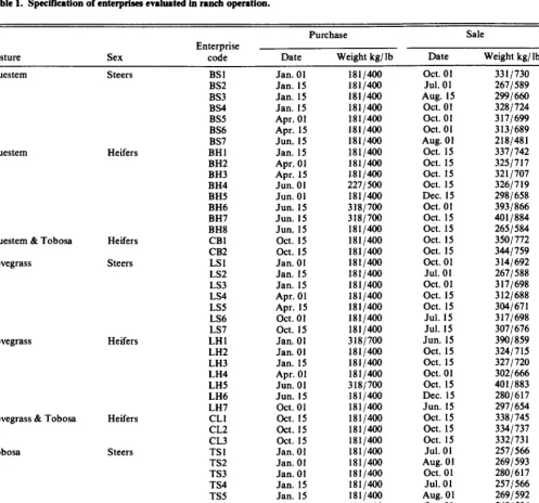
A profitable alternative may be available when high producing grasses such as weeping lovegrass (Eragrostis curvula) and old world bluestem (Bothriochloa ischaemum var. ischaemum) are established on a portion of ranch acreage, altering the production period and exploiting the seasonal cattle price pattern. The objectives of this study were to identify feasible alternative purchase and sale dates for stocker cattle enterprises on lovegrass, bluestem, and tobosagrass pastures in the Southern High Plains/ Rolling Plains and determine the combinations of enterprises which maximize profits for ranches in the region. Objectives did not include deter- mination of optimum acreages of the various pastures, but annual- ized establishment costs for improved pastures were included in enterprise costs. The optimum combinations of enterprises were evaluated on a model ranch which has the improved pastures established.

Several studies with related emphases have been done. Angirasa et al. (198 I) evaluated a related question of fall and spring calving in East Texas. Leistritz and Qualey (1975) analyzed use of various forages and alternative sale dates of calves in a cow-calf operation in southwestern North Dakota. Lance et al. (1974) studied the profitability of winter and summer stocker and cow-calf enterprises for the southeastern U.S. and concluded that a combination of summer cow-calf and winter stockers was the optimal production system. Woodworth (1973) determined the optimal distribution of steers and heifers between 2 types of pastures. Kennedy (1972) described a method to determine optimal production possi- bilities for stocker enterprises which included using capital budgets for a wide range of management practices. That approach was used

The authors are professor and former research assistant, Agricultural Economics Department, and professor, Range and Wildlife Management Department, Texas Tech University, Lubbock 79409.

Texas Tech University College of Agricultural Sciences Publication No. T-l-236. The authors wish to thank R.P. Kennedy, R.T. Erwin, R.E. Sosebee, R.H. Hart, and two anonymous reviewers for their comments and suggestions.

Manuscript accepted 8 December 1986.

JOURNAL OF RANGE MANAGEMENT 40(3). May 1987

in this study. Bentley and Shumway (1981) showed that forecasts of patterns in beef prices could be incorporated in profit maximiz- ing ranch management decisions.

Methods

The Texas Tech Experimental Ranch, located at Justiceburg, Texas, in the eastern part of Garza county, has 397 ha (980 ac) of * productive land, consisting of pastures of weeping lovegrass, old world bluestem, and native tobosagrass (Hilaria mutica). It was used as the model ranch for this analysis. The bluestem and lovegrass pastures each contain 30 ha (75 ac). The tobosagrass area, 336 ha (830 ac), was treated with herbicides in 1983 for honey mesquite (Prosopis glandulosa), was burned in 1981, 1982, and 1983 (I/ 3 each year), and has about 10% canopy cover. All 3 pastures have rotation grazing systems using 6 paddocks in each pasture. The herd on tobosagrass is rotated weekly while the herds on lovegrass and bluestem are rotated by decision as dictated by pasture conditions. The estimated annual grass production available for grazing, based on clipping samples from these and other sites, was 3,226 kg/ ha (2,880 lb/at) for the bluestem, 3,584 kg/ ha (3,200 lb/at) for the lovegrass, and 806 kg/ha (720 lb/at) for the tobosagrass. Fertilized bluestem commonly yields 4,000 to 4,500 kg/ ha in the area. Similarly, lovegrass yields from 4,500 to 5,000 kg/ ha and unfertilized tobosagrass 1,300 to 1,600 kg/ ha. These values assume that at least 900 kg/ ha (800 lb/at) will be left on bluestem and lovegrass pastures and that 540 kg/ ha (480 Ib/ac) will be left on tobosagrass pastures to allow for maintenance of stand. The production estimate for the tobosagrass site is conditioned on pres- cribed burning on a cycle of approximately 5 years.

The enterprises examined consisted of stocker steers and stocker heifers. The enterprises differed in the purchase weights, purchase and sale dates of the cattle, and in types of forage consumed. Alternative purchase and sale dates were selected from 566 enterprises (Nance et al. 1985) on the basis of profitability of the enterprise, affected by rate of weight gain and price spreads between purchase and sale, and technical feasibility, affected by forage availability in different months. Weight gains for each enterprise were based on unpublished experimental data and experience from operating the ranch. Considerable data compare steers and heifers before weaning and in the feedlot phases of cattle production, but little data exist for the stocker pasture and range phase. However, from the relatively few pasture studies conducted with stockers, little difference exists between weight gains of steers and heifers for this phase. The only published comparative data found confirmed this and was from Kessler et al. (1951) in a Kansas study. Also Snapp (1949) and Morrison (1949) report from several Midwestern feedlot studies that if steers and heifers are marketed when the finish required for the respective sex is attained, heifers gained as well or better than steers. However, when both sexes were fed the same length of time the steers outperformed the heifers. For lack of a better guide, this analysis assumed the same daily gain from steers and heifers. There are, however, differences in rate of weight gain from both steers and heifers in different months; cattle on pasture gain more rapidly during the spring, summer, and fall periods than during the winter months even with supplemental feeding in the winter.

Enterprise budgets constructed for each alternative strategy and

(10)

procedure are described in Nance et al. (1985). The budgets were also modified to determine costs and returns for alternative levels of cattle prices.

A linear programming model was constructed to determine the combination of enterprises for maximum net revenue with high, low, and average cattle prices. Profitability for each enterprise was indicated by its residual returns to land and management.

prises using lovegrass during the April 15-May I5 period were rotated to tobosagrass pastures for this period to protect the lovegrass productivity. Eight steer and six heifer enterprises were considered on tobosagrass. Livestock stocking rates were derived from median forage production and utilization values obtained from relatively intense management of pastures in west Texas by Texas Tech University researchers.

Seven stocker steer and ten stocker heifer enterprises on blue- The linear programming model used to maximize net ranch stem were evaluated in the model (Table 1). Two heifer enterprises, income included the 48 enterprises (Table 1) plus 36 transfer activi- CBl and CB2, were purchased October 15 and grazed initially on ties. The transfer activities transferred consumed grass from one tobosagrass, then rotated to bluestem on June 1 and 15, where they month to the next. The limiting resources were land area in each of remained until sold. Seven stocker steer and ten stocker heifer the grasses and labor. Allocation of land was based on daily grass enterprises were considered for the lovegrass. Three heifer enter- consumption per head for each month for each enterprise. The prises, CLl-CW, were grazed on tobosagrass from their purchase total amount of grass available in any month was the sum of grass date until May 15, June 1, and June 15, respectively, then rotated produced and grass transferred into that month, less the senescence to lovegrass for the duration of the production period. All enter- and trampling losses.

Table 1. Specification of enterprises evaluated in ranch operation.

Pasture Sex

Enterprise code

Purchase Sale

Net revenue’ Date Weight kg/ lb Date Weight kg/ lb %/hd/yr Bluestem Bluestem Steers Heifers BSI BS2 BS3 BS4 BS5 BS6 BS7 BHl BH2 BH3 BH4 BH5 BH6 BH7

Bluestem 8t Tobosa

Lovegrass

Heifers

Steers

Lovegrass Heifers

Lovegrass & Tobosa Heifers

Tobosa Steers

BH8 CBl CB2 LSl LS2 LS3 LS4 LSS LS6 LS7 LHI LH2 LH3 LH4 LHS LH6 LH7 CL1 CL2 CL3 TSI TS2 TS3 TS4 TS5 TS6 TS7 TS8 THl TH2 TH3 TH4 THS TH6

Tobosa Heifers

Jan. 01 Jan. 15 Jan. 15 Jan. 15 Apr. 01 Apr. 15 Jun. I5 Jan. 15 Apr. 01 Apr. 15 Jun. 01 Jun. 01 Jun. 15 Jun. 15 Jun. 15 Oct. 15 Oct. 15 Jan. 01 Jan. 15 Jan. 15 Apr. 01 Apr. 15 Oct. 01 Oct. I5 Jan. 01 Jan. 01 Jan. 15 Apr. 01 Jun. 01 Jun. 15 Oct. 01 Oct. 15 Oct. 15 Oct. 15 Jan. 01 Jan. 01 Jan. 01 Jan. 15 Jan. 15 Apr. 01 Oct. 15 Jan. 15 Jan. 01 Jan. 15 Jan. 15 Apr. 01 Oct. 01 Oct. 15

181/400 Oct. 01 331/730 25.03

181/400 Jul. 01 2671589 15.72

lSl/400 Aug. 15 2991660 22.19

181/400 Oct. 01 3281724 34.28

lSl/400 Oct. 01 3171699 38.22

181/400 Oct. 01 3131689 35.37

181/400 Aug. 01 218/481 14.44

181/400 Oct. 15 3371742 63.49

181/400 Oct. 15 3251717 65.63

181/400 Oct. 15 3211707 64.79

2271500 Oct. 15 3261719 40.35

181/400 Dec. 15 2981658 18.64

318/700 Oct. 01 3931866 20.49

318/700 Oct. 15 4011884 18.21

181/400 Oct. 15 2651584 10.66

181/400 Oct. 15 3501772 79.01

181/400 Oct. 15 3441759 73.27

181/400 Oct. 01 3141692 23.21

181/400 Jul. 01 2671588 18.74

181/400 Oct. 01 3171698 42.38

181/400 Oct. 15 312/688 19.48

181/400 Oct. 15 304/671 15.93

181/400 Jul. 15 3171698 9.98

181/400 Jul. 15 3071676 8.65

318/700 Jun. 15 3901859 11.70

181/400 Oct. 15 3241715 53.46

181/400 Oct. 15 3271720 65.28

181/400 Oct. 01 3021666 23.29

318/700 Oct. 15 401/883 18.52

181/400 Dec. 15 280/617 12.00

181/400 Jun. 15 2911654 6.26

181/400 Oct. 15 3381745 72.16

181/400 Oct. 15 3341737 76.38

181/400 Oct. 15 3321731 68.82

181/400 Jul. 01 2571566 24.21

181/400 Aug. 01 2691593 37.44

181/400 Oct. 01 2801617 24.89

181/400 Jul. 01 2571566 33.06

181/400 Aug. 01 2691592 46.36

181/400 Oct. 01 2691594 29.01

181/400 Jul. 15 2701596 23.40

181/400 Jul. 15 2611576 38.21

318/700 Jun. 15 388/855 50.22

318/700 Jun. 15 388/855 51.73

2271500 Oct. 15 3271721 55.94

181/400 Jun. 15 2691594 26.35

181/400 Jun. 15 2631580 9.45

181/400 Jun. 15 2691575 12.38

(11)

Labor requirements for each enterprise were specified on a per month basis. Estimates of labor required were from Texas Agricul- tural Extension Service/Texas Agricultural Experiment Station (1984) livestock enterprise budgets for the region. An additional .04 hr of labor per head was used in the month when animals were purchased to account for vaccination, branding, and associated activities. The months when the cattle were sold, as well as when the cattle were rotated from one site to another, had an additional .02 hr more labor per head added. Labor available in each month was the number of daylight hours in that month, or the labor of one man working daylight to dusk each day.

Three model solutions were obtained, one each for average, high, and low cattle prices. Average prices were 7-year averages of prices for each weight group for each month (Nance et al. 1985). High and low cattle prices were 1 standard deviation above and below the average, respectively. Because price variability is not constant across months, weight groups, or sex, net returns of the various enterprises did not move proportionately.

Results

A result common to all solutions was that labor requirements never exceeded the total labor available. However, additional labor was hired for veterinary and processing activities during the months of purchasing and selling.

The optimal solutions are summarized in Table 2. The average cattle price model yielded a total annual net return over variable costs of $19,833 on the 397 ha and net returns to land and management of $14,549 after subtracting the $5,284 fixed costs of the ranch. The bluestem site’s cattle production was limited to 65 head of heifers by the grass produced and transferred into August, all of which was consumed. The value of the dual activity (the activity’s shadow price) for the bluestem site was $.0441/kg (.02/lb); an additional kilogram of bluestem grass would increase net income by %.0441. An additional hectare of the bluestem would have increased net ranch returns by $142 per year ($.0441/ kg X 3,226 kg grass/ ha/ yr). The additional hectare would produce net income from almost 2 heifers.

The lovegrass site was limited to 61 heifers by the grass available in March. The value of the dual activity for this site was $.033 1 /kg ($.015/ lb), indicating that an additional hectare of lovegrass would be worth $119 annually. The tobosagrass site was limited to 225 heifers by the grass available in April. The shadow price was $.0441/kg ($.02/lb) and the value of an additional hectare of tobosagrass was $35.58 ($14.40/ac).

In the average cattle price model, $70,241 of annual operating

Table 2. Optimal ranch plans under three cattle price levels.

capital (to purchase cattle, fedd, supplies, and other operating cost items) was required for the enterprises. The operating capital for the lovegrass enterprise was larger than for bluestem and tobosagrass. The extended duration of grazing on lovegrass required more supplemental feeding, fertilization, and interest cost (Nance et al. 1985).

The optimal solution for the high cattle price model yielded a net return over variable costs of $22,881 and a net return to land and management of $17,597,15 and 2 1% above the average price model solutions, respectively. The solution consisted of 282 steers on bluestem, 61 heifers on lovegrass, and 225 heifers on tobosagrass, and required $79,083 of operating capital.

Bluestem use was limited to 282 head by the grass available in July. The value of additional bluestem grass was $.044/kg or $142/ha annually. Allocation of the lovegrass and tobosagrass did not vary from the average price model, but their net returns did. The shadow price for lovegrass fell to $.022/kg ($.Ol/ lb) of grass and $461 ha ($18.72/ac) annually. This happened because increased cattle prices caused per head net revenue to decline on lovegrass and increase on tobosagrass.

With low cattle prices, the optimal solution resulted in net returns over variable costs of $22,593, 14% over those for the average price model, and net returns to land and management were 19% greater. These returns were generated with 65 heifers on bluestem, 61 heifers on lovegrass, and 201 steers on tobosagrass and required $52,135 of operating capital. Use of the bluestem and lovegrass sites for the low price model did not vary from the average price model, but the value of an additional kilogram (ha) of bluestem increased to $.0441(%158) annually. The 201 head on tobosagrass was limited by grass available in April. The shadow price of an additional kg (ha) of tobosagrass was $.0441 ($36) annually in the low price model.

The optimal ranch use with average cattle prices is production of heifers on all sites. With high cattle prices, the optimal solution substitutes steers for heifers on the bluestem site. Low cattle prices results in substitution of steers on tobosagrass and the same use of the other sites as with average cattle prices.

Comparison of results with average, high, and low cattle prices shows that income is highly dependent on the buy-sell price differ- entials, not on absolute price levels. These results also indicate that variation in cattle prices, if predictable, do not lower net returns if the enterprise mix can be varied in response to price changes. Net returns were greater with both high and low cattle prices than with average prices. Increased profits with low cattle prices resulted from a decrease in purchase prices relative to sale prices due to

Cattle price level

Average

Pasture

Bluestem Lovegrass Tobosa

Number (head)

65 61 225

Purchase Sale

Weight Price Weight Price Net revenue2

Sex’ kg(lb) a/kg (a/lb) Date kg(lb) a/kg (a/W Date % H 181(400) 146.85(66.61) Apr. 15 321(707) 136.38(61.86) Oct. 15 4,212 H 181(400) 134.15(60.85) Jan. 15 327(720) 136.38(61.86) Oct. I5 3,982 H 318(700) 131.44(59.62) Jan. 15 388(855) 142.44(64.61) Jun. 15 11,639

High

Total 351

Bluestem 282 s

Lovegrass 61 H

Tobosa 225 H

Low

Total

Bluestem Lovegrass Tobosa

568

65 H

61 H

201 S

19,833 181(400) 189.57(85.99) Jun. 15 218(481) 185.9q84.34) Aug. 01 4,289 181(400) 162.37(73.65) Jan. 15 327(720) 148.81(67.50) Oct. 15 3,141 318(700) 144.18(65.40) Jan. 15 388(855) 157.92(71.63) Jun. 15 15,451

22,88 1

181(400) 118.08(53.56) Apr. 15 321(707) 123.9q56.22) Oct. 15 5,271 181(400) 105.93(48.05) Jan. 15 327(720) 123.9q56.22) Oct. 15 5,097 181(400) 125.8q57.08) Jan. 15 269(592) 128.57(58.32) Aug. 01 12,225

Total 327 22.593

IH = Heifers, S q Steers

*Net returns over variable costs.

(12)

larger standard deviations for prices of lighter cattle than for heavier cattle. Furthermore, low cattle prices decreased operating capital requirements. However, if the ranch manager is to benefit from high or low cattle prices, he must have reliable forecasts of the movement of prices and alter his production strategy to exploit it. The results of management choices of the high, average, of low cattle price strategies with various outcomes-high, average, or low cattle prices-actually occurring are shown in Table 3. If an

Table 3. Net ranch incomes of various cattle price outcomes under various price strntegies.

Price strategy

Outcomes

High prices Average prices Low prices

---dollars---

High prices 17,517 14,409 I i ,494 Average prices 16,460 14,549 12,910

Low prices 7,421 12,228 17,309

average cattle price strategy is followed and average cattle prices actually occur, the ranch makes a net income to land and management of % 14,549. If the average price strategy is followed and low prices result, the net ranch income (return to land and management) is $12,910, a reduction of $1,639 from the average price outcomeand a reduction of $4,339 (%17,309-%12,81O)from thelow price strategy-low price outcome. Table 3 can be used in the above illustrated manner to evaluate potential losses and gains from various strategies. In general, comparison of the potential outcomes identifies the value of reliable cattle price outlook informa- tion to ranch managers.

The use of improved pastures in ranch production systems coupled with unconventional marketing techniques of seasonal buying and selling activities can increase the profitability of stocker cattle operations. Production of heifers is more profitable than production of steers with average market price differences and the production responses used in this study.

The study also indicates that larger ranch profits can be made

with both high and low cattle prices than with average cattle prices if (a) price levels are predictable and (b) ranch production is modified to take advantage of the price movements. The analysis included variations in cattle prices, but normal weather was assumed throughout. Therefore, price risk was recognized but production risk was not.

Literature Cited

Anginsa, A.K., R. Shumway, T.C. Nelsen, and T.C. Cartwrighbt. 1981. Integration, risk, and supply response: a simulation and linear pro- gramming analysis of an east Texas cow-calf producer. So. J. Agr. Econ. 3:89-91.

Bentley, E., and CR. Shumway. 1981. Adaptive planning over the cattle cycle. So. J. Agr. Econ. 13:139-148.

Kennedy, J.O.S. 1972. A model for determining optimal marketing and feeding policies for beef cattle. Amer. J. Agr. Econ. 23: 147-159.

Kessler, F.B., L.C. Aicher, and F.E. Meenen. 1951. Grass utilization and pasture management investigations for 1946-50. Kansas Agr. Exp. Sta.. Circ. 276.

Lanee, C.G., G.V. Caivert, and W.A. Griffey. 1974. Alternative cow-calf and stocker production systems in the Georgia Piedmont area. J. Range Manage. 27:344-346.

Leistritx, B., and N.J. Quaiey. 1975. Economics of ranch management alternatives in southwestern North Dakota. J. Range Manage. 28:349-352.

Morrison, F.B. 1947. Feeds and feeding-a handbook for the student and stockman. The Morrison Publishing Co.

Nance, J.D., B.E. Dahi, and D.E. Ethridge. 1985. Stocker cattle costs and returns for selected purchase and sale dates on different forage pastures, southern plains. College of Agr. Sci., Texas Tech Univ., Pub. No. T-l -23 1, December.

Snapp, R.R. 1949 (3rd cd.). Beef cattle-their feeding and management in the corn belt states. New York: John Wiley and Sons, Inc.

Texes Agricultural Extension Service and Texas Agricultural Experiment Station. 1984.1985 Texas crop and livestock budgets. Texas High Plains Region III, November.

Texas Crop and Livestock Reporting Serviee. 1984. Texas agricultural cash receipts, prices received and paid by farmers, 1983. Texas Depart- ment of Agriculture, Marketing Division, and Stat. Reporting Serv., U.S.D.A., Government Printing Office, Washington, D.C.

U.S. Dept. of Agr. 1984. Agricultural statistics, 1983. Stat. Reporting Serv., Government Printing Office, Washington, D.C.

Woodworth,B.M. 1973.Optimizing the calf mix on range lands with linear programming. J. Range Manage. 26:175-178.

JRM

X-year

Index

Now Available

The index to volumes 1 through 35,1948 to 1982, is now available. Edited by Elbert H. Reid, the publication contains a subject and author index with keywords and taxons followed by a chronological list of all articles printed in the journal from 1948 to 1982. Using the two lists enables the reader to locate the subject of interest and identify the articles without going to the magazine itself.

The index is 100 pages8 l/2 by 11 and is perfect bound and sewed. It can be purchased postpaid for $10.00

(US) from the Society for Range Management, 1839 York Street, Denver, Colorado 60206.