International Journal of Innovative Research in Science, Engineering and Technology
An ISO 3297: 2007 Certified Organization Volume 6, Special Issue 5, March 2017
National Conference on Advanced Computing, Communication and Electrical Systems - (NCACCES'17)
24th - 25th March 2017
Organized by
C. H. Mohammed Koya
KMEA Engineering College, Kerala- 683561, India
A Novel Method for Computation of Air Data
Parameters using Nose Cap Pressure
Distribution
Dr M Jayakumar1,N Remesh2, Abhay Kumar3, Dr S Swaminathan4, Dr K Sivan5 & Prof. M A Ramaswamy6
Dy. Project Director, Rlv-Td, VSSC, Indian Space Research Organization (ISRO), Thiruvananthapuram, India1
Scientist/Engineer ‘Sg’, Fmd, VSSC, Indian Space Research Organization (ISRO), Thiruvananthapuram, India2
Group Director, AFDG, Aeronautics Entity, VSSC, ISRO, Thiruvananthapuram, India3
Deputy Director (Rtd), Aeronautics Entity, VSSC, ISRO, Thiruvananthapuram, India4
Director, VSSC, ISRO, Thiruvananthapuram, India5
Professor (Retd.), Indian Institute Of Science, Bangalore, India6
ABSTRACT: Hypersonic re entry vehicles which encounter high thermal environment normally utilize the concept of Flush Air Data System (FADS) to estimate air data parameters like Mach number, angles of attack and sideslip, free stream static pressure and dynamic pressure. FADS employed in many of the so far reported programs uses a simplified aerodynamic model to relate surface pressure measurements to air data states and an estimation algorithm for air data computation. In this paper, a novel method for air data computation for a wing body re entry vehicle is presented. The method, based on the physical nature of the flow, extracts air data from pressure distribution over the nose cap of the vehicle. The location of maximum pressure at the nose cap provides an indication of angle of attack and the second derivative of pressure variation with respect to port location gives an indication of Mach number. Knowing the stagnation pressure, free stream pressure and dynamic pressure can be estimated using gas dynamics relations. Measured pressures at different locations around the nose cap are used for this study. The proposed scheme of air data computation is tested along a simulated re entry trajectory profile from Mach number 2.5 to 0.2. The maximum algorithm errors in angle of attack and Mach number are found to be 0.3 deg and 0.1 respectively, which is comparable to that of other currently existing FADS algorithms. With the present method, real-time onboard implementation of the air data computation is easy and it is independent of aerodynamic model, which is a definite advantage compared to most of the reported FADS algorithms.
KEYWORDS: FADS, EMI, EMC, RS03, CS01, CS02, CS06
I. INTRODUCTION
Mission management of hypersonic reentry vehicles, including Reusable Launch Vehicle (RLV), calls for maneuvering of the flight along an optimum profile, limiting the vehicle structural loads and thermal environment to manageable levels. Accurate and near real time knowledge of air data parameters like Mach number, angles of attack, angle of sideslip and free stream static pressure is essential for this purpose. These air data parameters find use in flight control systems and are also required for overall mission management.
nature of the flow. Systems based on inertial measurement cannot directly take care of local wind effects. So, hypersonic flying vehicles essentially resort to the concept of Flush Air Data System (FADS) [3].
Design and development of FADS is an involved task considering the thermal environment and complexity in generation of air data states in near real time. In FADS, the air data parameters need to be estimated using pressure measurements from orifices flushed with the surface of the vehicle. This is an inverse problem. Therefore we need an explicit expression for the pressure at a port location, as a function of angle of attack, sideslip, dynamic pressure (or Mach number) and free stream pressure. Available option is to use a simple aerodynamic model, which relates the air data parameters to the measured pressure and do calibration using wind tunnel data for variation in Mach number, geometry, etc. The aerodynamic model should be capable of solving the inverse problem, viz., to deduce the vehicle air data states from surface pressure measurements. It is also required that the proposed aerodynamic model needs to capture the salient features of the flow, and is valid over a large Mach number range from hypersonic to subsonic. Further it must be simple enough to be inverted in real-time so that the air data parameters can be extracted on-board.
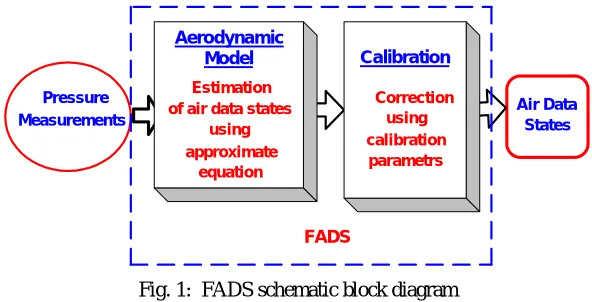
Most of the presently reported FADS algorithms use simple aerodynamic models, which relate the air data parameters to the measured pressures [3, 4, 5]. The typical computational block diagram of FADS is shown in fig1. The aerodynamic model is postulated as a combination of a simple potential flow model on a sphere, and modified Newtonian flow theory for blunt objects in hypersonic flow [3, 4, 6]. As the aerodynamic model is not exact, it needs to be supplemented with calibration parameters [7, 8, 9]. Various reported papers in FADS differ in the methods used for estimation of air data parameters utilizing the simplified aerodynamic model. Different estimation algorithms like nonlinear regression, triples, neural network, etc., are reported for FADS air data estimation [10, 11, 12, 13, 14, 15].
Pressure Measurements
Air Data States Aerodynamic
Model
Estimation of air data states
using approximate
equation
Calibration
Correction using calibration parametrs
FADS
Fig. 1: FADS schematic block diagram
In this paper, an attempt is made to use the trends in pressure distribution over the spherical nose of the vehicle to estimate the angle of attack, Mach number, dynamic pressure and free stream pressure based on the physical nature of the flow. The next section details the FADS concepts currently used and then the proposed ideas are discussed. The details of the proposed FADS algorithm are provided subsequently. Application for a typical RLV case and simulation, results and conclusions are presented at the end of the paper.
II. EXISTING FADS ALGORITHMS
All existing FADS algorithms use an aerodynamic model, which relates the air data parameters to the measured pressures. This model as mentioned earlier, is derived as a splice of the closed form potential flow solution for a blunt body, applicable at low subsonic speeds; and the modified Newtonian flow model, applicable at hypersonic speeds [3]-[5]. Both potential flow and modified Newtonian flow describe the measured pressure coefficient in terms of the local surface incidence angle. To blend the two solutions over a large range of Mach numbers, a calibration parameter (ε) is devised. The aerodynamic model is of the form
q [cos ε sin ] P
P 2 i
i 2 c
i (1)
In equation 1, i is the flow incidence angle between the surface normal at the ith port and the vehicle velocity vector.
The incidence angle is related to the effective angle of attack, (αe) and angle of sideslip, (βe) at the port location, port
cone angle (i) from vehicle body axis and clock angle (i) around the nose cap axis as given in equation 2 [3].
i e e
λ sin sin β sin
λ cos β cos α cos cos
This equation is derived from the dot product of velocity vector around the nose cap and the port surface normal vector. If the nose cap axis orientation is different from body axis then port cone angle (i) is replaced with port geometrical
angle () in the above equation. If body axis coincides with nose cap axis, then =. Various estimation algorithms are
used in obtaining αe, βe, Mach number etc. from the above model.
The first estimation algorithm capable of real-time operation was developed at NASA Dryden during the late 1980s for the F/A-18 High Alpha Research Vehicle (HARV) program [9]. It used a Nonlinear Regression (NR) algorithm, which is similar to SEADS [5] (Shuttle Entry Air Data System) algorithm. Nonlinear regression algorithm had problems with algorithm stability in the transonic and supersonic flight regimes and in presence of undetected sensor failures [4]. To overcome problems encountered using the NR algorithm, a new solution algorithm, namely ‘Triples’ was developed for the X-33, X-34, and X-38 demonstration vehicles [3].
This solution algorithm, works with strategic combinations of three pressure sensor readings to analytically decouple the angle-of-attack and angle-of-sideslip computations from the Mach number and static pressure calculations.
Another method of air data estimation is to use a trained artificial neural network [13, 14, 15, and 16] with large sets of data that relate air data parameters to nose pressures. The data bank can be obtained from flight tests, computational results, or ground based experimental data. Reliability and accuracy of neural networks is difficult to quantify, and massive amounts of data are generally required for the network to accurately learn the relationships between air data parameters and surface pressures.
III. PROPOSED FADS ALGORITHM
The proposed FADS algorithm makes use of the trends in pressure distribution over the nose cap to estimate the air data parameters. The pressure ratio between each measured port pressure (P) and the maximum measured pressure (Pm) among the ports is generated and its variation with port location (
) is used for finding the angle of attack and Mach number. The novelty of this method is that it does not require the aerodynamic model for air data computation. All reported FADS algorithms use an aerodynamic model for air data estimation. Another advantage of the proposed scheme is that it requires only a simple table look up interpolation and sorting of 4 pressure data. Hence it requires minimal computational time and effort compared to other algorithms which are mentioned in the previous section. In this paper this novel method of computing air data parameters using the measured pressure pattern over the nose cap at different port locations is presented.Aerodynamic characterization of a spherical surface
For a spherical surface, the coefficient of pressure variation along the vertical plane is as follows.
Subsonic flow
2 sin 4 9 1
Cp
(3) Hypersonic flow (Modified Newtonian flow model)
2 maxcos Cp
Cp (4)
where is the flow impact angle on sphere (fig 2).
V
CPmax CPmax CPmax
Port surface normal
Fig 2: Flow impact angle on a sphere
-60 -40 -20 0 10 20 40 60 -1
-0.5 0 0.5 1 1.5 2
Theta (Port location) (deg)
C
o
e
ff
ic
ie
n
t
o
f
P
re
s
s
u
re
Hypersonic
AOA 10 deg AOA 0 deg
Subsonic
AOA 0 deg AOA 10 deg
Fig. 3: Cp variations for flow over a Sphere
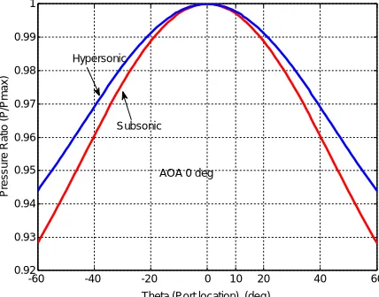
The maximum surface pressure occurs at the stagnation point and the pressure decreases away from the stagnation point. Variation of local pressure and maximum pressure ratio (P/Pmax) with port location () for a sphere for subsonic
and hypersonic cases for 0 & 10 deg angles of attack (AOA) are shown in figs 4 & 5 respectively.
-60 -40 -20 0 10 20 40 60
0.92 0.93 0.94 0.95 0.96 0.97 0.98 0.99 1
Theta (Port location) (deg)
P
re
s
s
u
re
R
a
ti
o
(
P
/P
m
a
x
)
Subsonic Hypersonic
AOA 0 deg
Fig. 4: Pressure ratio vs port location for Sphere for angle of attack 0 deg
-60 -40 -20 0 10 20 40 60
0.91 0.92 0.93 0.94 0.95 0.96 0.97 0.98 0.99 1
Theta (Port location) deg
P
re
s
s
u
re
R
a
tio
(
P
/P
m
a
x
)
Subsonic Hypersonic
AOA 10 deg
From the above data for an isolated spherical body (fig 2), it is obvious that the maximum pressure occurs at angle =0 which corresponds to the stagnation point. If we are able to identify the exact point at which stagnation or maximum pressure occurs, the angle that the surface normal makes with the body axis will be angle of attack.
From figs 4 & 5 it can be seen that the curvature of the plot of P/Pmax Vs port location at the maximum (stagnation)
pressure point are different for subsonic flow and hypersonic flow. It is therefore hypothesized that the curvature of the variation of P/Pmax with at this stagnation point would be a function of Mach number. This aerodynamic property can
be used to find the angle of attack of the body.
Application of the concept to RLV FADS
For practical reentry vehicles, though a spherical nose cap can be provided, the shape of the body after the nose cap cannot be made symmetrical with respect to the nose cap as it is decided by aerodynamic requirements. Nevertheless, it was felt that this idea could be extended to such bodies also with slight modifications, using calibrated data from wind tunnel tests. The application of these concepts for a typical RLV is explained below.
RLV Nose body
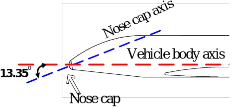
The RLV blunt nose body under consideration (fig 6) is of complex shape and the pressure variation in the region of stagnation point can be slightly different from that of a sphere. The nose body considered consists of an inclined spherically blunted conical body attached to the forward part of fuselage. The nose body is inclined to the fuselage by 13.35 deg as shown in fig 6. The pressure port locations are on the spherical cap and hence the proposed idea has been applied in this case, with modification using measured data from wind tunnel tests.
13.350
No
se
cap
ax
is
Vehicle body axis
Nose cap
Fig. 6: Vehicle axis & Nose cap axis
FADS port geometry
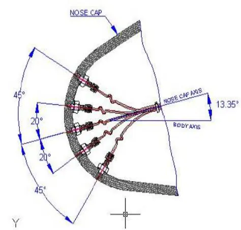
The geometrical angle (), cone angle () and clock angle () for RLV nose cap pressure port locations are shown in fig 7. Cone angle for a pressure port is the angle between the port surface normal and the nose body axis. Clock angle is the clockwise angle looking aft around the axis of symmetry starting at the bottom of the nose body. Fig 7 also shows the angle of attack and sideslip. Fig 8 shows the enlarged view of nose cap region showing the port location with respect to body axis and nose cap axis and the angle between them.(13.35 deg in this case).
Fig. 8: FADS port location with respect to body axis and nose cap axis
The relationship between θ & λ for ports in the vertical meridian is as follows
λ = 13.35 – θ (5)
FADS configuration used in this study makes use of nine pressure ports arranged in a crucifix fashion as shown in fig 9 [17, 18].
In this paper, ports on the vertical meridian (port number 1, 2, 5, 8 & 9) of RLV nose cap is considered for air data computations. Ports on the horizontal meridian (port number 3, 4, 5, 6 & 7) can be used to derive angle of sideslip, which is not addressed in this paper. The geometrical angle , cone and clock angle of the ports in the vertical meridian are given in table 1.
For on-board real-time applications, measured absolute pressure of accuracy of 150 to 250 Pa is used [19, 20]. For fault tolerance, Triple Modular Redundancy (TMR) scheme is used for the pressure sensors at a port. In this scheme, three functionally identical sensors are used at each port. Faulty sensors are detected by cross comparing the three sensor outputs. If all three sensors are working, the median of the value provided by the three sensors is used for computation. In case any one of the sensors is faulty, the average value of the two working sensors is used for computation.
Table 1: Geometrical angle, cone angle and clock angle of FADS vertical ports
Port
Id
Geometrical
Angle ()
from nose cap
axis
(deg)
Cone
angle ()
from
body axis
(deg)
Clock angle
() around
nose cap
axis)
(deg)
1 45 -31.65 180
2 20 -6.65 180
5 0 13.35 0
8 -20 33.35 0
Fig. 9: Pressure ports on RLV nose cap
For on-board real-time applications, measured absolute pressure of accuracy of 150 to 250 Pa is used. For fault tolerance scheme, Triple Modular Redundancy (TMR) scheme is used for the pressure sensors at a port. In this scheme, three functionally identical sensors are used at each port. Faulty sensors are detected by cross comparing the three sensor outputs. If all three sensors are working, the median of the value provided by the three sensors is used for computation. In case any one of the sensors is faulty, the average value of the two working sensors is used for computation.
Pressure data for RLV port geometry FADS Wind tunnel Data
Extensive wind tunnel tests were done for RLV model (1:8 scale model) to get the pressure coefficient at different port locations over the nose cap. Coefficient of pressure (Cp) data for FADS ports are obtained from wind tunnel test for Mach number range 0.2 to 2.5 and alpha range from –4 to 14 deg in steps of 2 deg. Cp variation for vertical meridian ports (1, 2, 5, 8 & 9) are shown in fig 10 & 11 for two typical Mach numbers of 1.1 and 2.0. The Cp data sets are presented for angle of attack ranging from –4 to 14 deg.
-0.5 0 0.5 1.0 1.5
-50 -40 -30 -20 -10 0 10 20 30 40 50
= -4
= -2
= 0
= 2
= 4
= 6
= 8
= 10
= 12
= 14 Mach number 1.1
Port location( - deg)
C
p
Fig. 10: Cp variation for vertical ports for M=1.1 Fig. 11: Cp variation for vertical ports for M=2
The required pressure information for analysis is derived from Cp data using wind tunnel free stream pressure and dynamic pressure. The maximum measurement error in wind tunnel derived Cp is about 0.02 and the corresponding error in pressure is within 25 to 30 Pa. This is repeatability error in measurement and the detailed explanation of the error is beyond the scope this paper.
Analysis of FADS pressure data
In this paper, computation of air data parameters using the pressure pattern over the nose cap with the measured pressure at different port locations is explored. The pressure ratio between each measured port pressure (P) and the maximum measured pressure (Pm) among the ports is generated and its variation with port location () is used for
-50 -40 -30 -20 -10 0 10 20 30 40 50 0.75 0.8 0.85 0.9 0.95 1 1.05 1.1 Mach 0.6 Theta (deg) P /P m a x AOA 14
A relationship between the location of maximum pressure and angle of attack () is derived using the measured Cp data. To obtain the pressure variation for vertical meridian ports, least square curve is fitted between θ and the ratio between the individual pressure and maximum of the measured pressure (P/Pm) for all vertical pressure ports. Ideally
the normalization should have been with respect to Pmax (maximum pressure at stagnation point). However Pmax being
not known apriori, the normalization is done with respect to Pm (the available maximum measured pressure).
The first derivative of P/Pm with respect to will be zero for the location at maximum pressure which will indicate the
angle of attack. The second derivative will give information on Mach number. It is also known that the second derivative of P/Pmvs θ will be highest near the stagnation point and it should reduce as we go away from it. To meet
these requirements, a 3rd order least square fit is needed
Pressure Variation -Least Square fit
A 3rd order polynomial of the form
3 3 2 2 1
0 a a a
a P P m (6) is considered as it is easier to obtain expressions for first and second derivatives. If Pmax is used for normalization, then the constant term a0 would be equal to 1.0. Using curve fit of P/Pm Vs. , Pmax is found. In addition is also found where it appears.
The first derivative and second derivative will be
3 2 2 2 2 3 2 1 6 2 3 2 a a P P a a a P P m m (7)
Using the condition that the first derivative of P/Pm with respect to will be zero at the location of maximum pressure
0=θ@ max pressure can be derived
3 3 1 2 2 3 2 max @ 0 2 3 2 1 3 3 3 3 2 0 a a a a a a a a a P P presure m (8) Where 0 corresponds to the angle, where the stagnation point occurs. Equation 8 has quadratic solution, which have
two roots. The root, which is closer to zero, provides the correct solution.
The third order curve fit & original data are shown in figs 12 & 13 for Mach 0.6 for two different angles of attack. The marker indicates the actual measured pressure ratio between the pressure at a port and maximum pressure among the ports. The solid line represents the curve fit using the pressure ratio. It is found that fitted curve matches closely with the wind tunnel data points. This shows the adequacy of third order fit for representing the pressure variation pattern (P/Pm vs ).
-50 -40 -30 -20 -10 0 10 20 30 40 50 0.55 0.6 0.65 0.7 0.75 0.8 0.85 0.9 0.95 1 1.05 Mach 0.6 Theta (deg) P /P m
AOA -4
Fig. 12: Third order fit for M 0.6, AOA -4deg Fig. 13:Third order fit for M 0.6, AOA 14deg
Computation of angle of attack
Here, a new term is introduced called derived angle of attack. The for which first differential is zero (0) at stagnation
0 0.3 0.6 0.9 1.2 1.5 2.4 2.1 2.5 0.65
0.7 0.75 0.8 0.85 0.9 0.95
Mach number
C
u
rv
e
f
it
li
n
e
a
r
C
o
e
ff
.
d = 13.35 - 0 (9)
With this derived angle of attack it is possible to compute the actual angle of attack. Using equation 5 and 9 it is clear that at stagnation pointdis same as λ. It was noted that the variation of derived angle of attack with actual angle
of attack for different Mach numbers is linear and this information is used to compute the actual angle of attack from the measured pressure. Therefore a linear fit is made with derived angle of attack (d) Vs. actual angle of attack ().
-10 -6 -2 2 6 10 14 18 20
-10 -5 0 5 10 15
A
c
tu
a
l A
O
A
Derived AOA
M=0.6 M=0.7 M=0.85 M=0.9 M=0.95 M=1.05 M=1.1 M=1.2 M=1.6 M=2.0 M=2.5
Fig. 14: Linear Fit for various Mach numbers
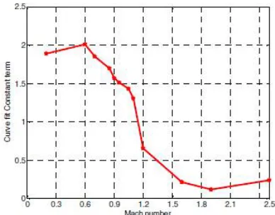
Fig. 15: Curve fit linear coefficient for various Mach numbers
Fig. 16:Curve fit constant term for various Mach numbers
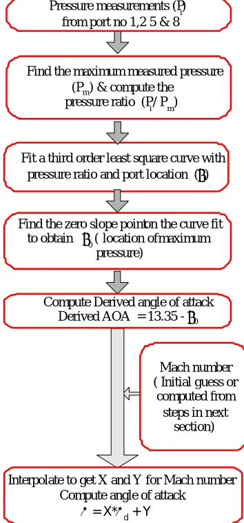
Find the zero slope pointon the curve fit to obtain 0 ( location ofmaximum
pressure)
Fit a third order least square curve with pressure ratio and port location (i)
Pressure measurements (Pi) from port no 1,2 5 & 8
Find the maximum measured pressure (Pm) & compute the
pressure ratio (Pi/ Pm)
Compute Derived angle of attack Derived AOA = 13.35 -0
Mach number ( Initial guess or
computed from steps in next
section)
Interpolate to get X and Y for Mach number Compute angle of attack
= X*d + Y
Fig. 17: Actual Angle of attack computation procedure
Computation of Mach number
The computation of the Mach number using the second derivative of pressure ratio is a novel idea. It is known that the second derivative of P/Pmvs θ will be highest near the stagnation point and it should reduce as we go away from it. The
location of the stagnation point in nose cap in real varying flight condition is not known. Hence with the maximum measured pressure and its location among the available pressure ports it is possible to derive the Mach number information. The accuracy of this procedure can be enhanced by adding more number of pressure ports (limited by geometric and plumbing line complexity) around nose cap and hence the location of maximum measured pressure will be same as stagnation pressure.
The information of the second derivative (equation 7) for 0(@peak pressure) from least square curve fit can be used to
compute Mach number. Mathematical derivations of the computation of second derivative of P/Pm with respect to at
0 (stagnation point) are as follows. Equation 6 is the curve fit between the pressure ratio and the port location angles
and it is repeated below.
3 3 2 2 1
0 a a a
a P
P
m
The above equation can be written as
) (
f P
P
m
(10)
It is required to get the second differential of pressure ratio with respect to at 0 (stagnation point). Therefore equation
10 can be represented as,
) ( max
max
f P P x P
P
m
Therefore ) ( max max f P P P P m (12)
Where Pmax is the stagnation point pressure (theoretical) and the available maximum measured pressure is Pm. The ratio
between these can be computed using equation 6 by substituting by 0
3 0 3 2 0 2 0 1 0
max a a a a
P P m (13) The second derivative of pressure ratio with respect to is
) ( '' max max 2 2
P f
P P P m (14)
This can be evaluated at 0
2 3 0 max max 2 2 6 2
P a a
P P
P m
(15)
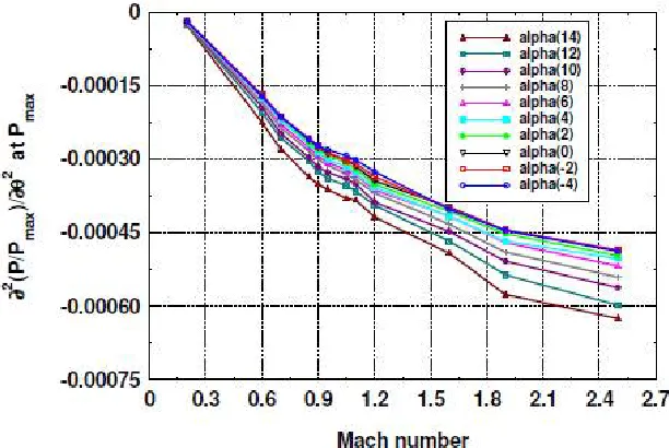
The value of second differential of pressure ratio with respect to at 0 is plotted with Mach number in fig 18. This
information is used as a table look up interpolation for the computation of Mach number.
Fig. 18: Second differentials of pressure ratio with respect to at Pmax
This second differential for different Mach numbers and angles of attack is in a tabular form. For the computed angle of attack, the second derivative of pressure ratio with respect to is obtained for all Mach numbers by linear interpolation and stored onboard. For the given flight condition, the measured pressure in the vertical meridian is fitted as a 3rd order curve with respect to . The second derivative of pressure with respect to at maximum pressure location for this curve is obtained. For this value, corresponding Mach number is obtained by linear interpolation from stored table. For this interpolated Mach number, the revised value of angle of attack is estimated using the procedure provided in the previous section. The procedure is repeated until convergence is achieved for angle of attack and Mach number. Normally it takes about 4 to 5 iterations for convergence.
Combined Steps to Compute Angle of attack and Mach number from Pressure measurement
The final algorithm to compute Mach number and angle of attack is provided in fig 19
Computation of free stream pressure (P) and dynamic pressure (Q)
NO Pressure data (Pi)
from port no 1,2 5 & 8
Find the maximum measured pressure (Pm) & compute the
pressure ratio (Pi/Pm)
Yes Compute Derived angle of attack
d
Compute the second derivative of P/P
m
with respect to at0
Second derivatives are linearly interpolated for all Mach number set with
computed angle of attack.
Interpolate to get Mach number for the second differential of real-time fitted curve of pressure
ratio with port location. Compute angle of attack
= X*d + Y
M and AOA Convergence ? Fit a third order least square curve with
pressure ratio and port angle (i)
0 (location of maximum pressure) Compute Pmaxat
Output Air data Parameters
Fig. 19: Steps for AOA and M computation
Subsonic flow: 2 1
01
2 1
1
M P
P (16)
Supersonic flow:
( 1)
2 1
) 1 ( 2 4
) 1
( 1 2
2 2 2 02
M
M M P
P (17)
The pressure ratio P/Pm computed using the curve fit equation at the location of @peak Pressure can be taken as P/Pmax. .
This ratio can be approximated as the pressure ratio between free stream static pressure and total pressure. Substituting Pmax for P01 or P02 in equation 16 or 17, Pcan be computed
Free stream dynamic pressure is computed using
Q=0.5*γ P M∞2 (18)
IV.VERIFICATION OF ALGORITHM BY SIMULATION
0 0.5 1.0 1.5 2.0 2.5 3.0
250 450 650 850 1050 1250
Estimated True
Trajectory Time(s)
M
a
c
h
n
u
m
b
e
r
for simulating the port pressures for FADS. In this Mach number range, is varied from 14 deg to 5 deg. FADS port pressures are simulated along the trajectory profile using an Inverse FADS simulator, which generates the FADS pressure data for testing and analysis. This simulator stores the wind tunnel derived coefficient of pressure (Cp) from the pressure ports as a function of Mach number (M), angle of attack (α) and angle of sideslip (β) in a table lookup. Depending on the required flight conditions, pressure coefficients for the nine ports are linearly interpolated in terms of
M, α and β respectively. The port pressures (Pi) are generated using pressure coefficients using trajectory dynamic
pressure (q) and atmospheric pressure (P).
These pressure data are used for the estimation of the air data parameters with the proposed FADS algorithm. The simulated pressure data sets are shown in fig 20. These pressure data sets were used for performance comparison of the present algorithm. The comparison results are shown in figs 21 to 28.
0 0.4 0.8 1.2
0 0.5 1.0 1.5 2.0 2.5
P8 P2 P5 P1 P9
Mach number
F
A
D
S
p
o
rt
P
re
s
s
u
re
(
b
a
r)
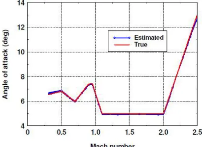
Fig. 20: FADS port pressure variation Fig .21: Angle of attack comparison
Fig. 22: Estimated AOA error Fig. 23: Mach number Comparison
-0.01x10⁵ 0.19x10⁵ 0.39x10⁵ 0.59x10⁵ 0.79x10⁵ 0.99x10⁵ 1.19x10⁵
0 0.5 1.0 1.5 2.0 2.5
Estimated True
Mach number
F
re
e
s
tr
e
a
m
P
re
s
s
u
re
(
P
a
)
-0.05 0 0.05 0.10 0.15
0 0.5 1.0 1.5 2.0 2.5
Mach number
M
a
c
h
n
u
m
b
e
r
e
rr
o
r
Fig 24: Estimated Mach number error Fig 25: Free stream pressure comparison
Fig 26: Estimated free stream pressure error Fig 27: Dynamic pressure Comparison
Fig 25 shows the free stream static pressure comparison and fig 26 shows the estimated free stream static error variation. Similarly dynamic pressure comparison is provided in fig 27 and dynamic pressure error is shown in fig 28. The maximum error in dynamic pressure and free stream pressure are within 1000 Pa (during subsonic regime).
Fig 28: Estimated Dynamic pressure error
V.CONCLUSION
In this paper, an alternate air data computational algorithm using pressure data around the nose cap is presented. The location of maximum pressure around the nose cap gives an indication of angle of attack and the variation of second derivative of the pressure pattern with port location provides insight into Mach number. Angle of attack (α) and Mach number (M) are computed from the pressure distribution obtained from the ports lying in the vertical meridian of the nose body of a Reusable Launch Vehicle (RLV). Air data parameters are computed along RLV trajectory using simulated pressure data and the results are compared with trajectory conditions. The maximum error in angle of attack is about 0.3 deg and in Mach number is about 0.1. Similarly the maximum error in dynamic pressure and free stream static pressure are within 1000 Pa. This computational scheme can be extended to compute sideslip angle from pressures measured along the horizontal pressure ports. This shall be the focus of future work.
VI.ACKNOWLEDGEMENT
The authors gratefully acknowledge Shri. C.S Harish, Deputy Project Director, Crew Escape System, HSP, VSSC, for carrying out the review of this paper and for the valuable editorial suggestions.
REFERENCES
[1] Ryan D. Eubank, Ella M. Atkins, and Stephanie Ogura. Fault Detection and Fail-Safe Operation with a Multiple-Redundancy Air-Data System. AIAA 2010-7855, AIAA Guidance, Navigation, and Control Conference 2 - 5 August 2010, Toronto,
[2] Georg Koppenwallner, Controlled Hypersonic Flight Air Data System and Flight Instrumentation. In Flight Experiments for HypersonicVehicle Development (pp. 17-1 – 17-30). Educational Notes RTO-EN-AVT-130, Paper 17. Neuilly-sur-Seine, France,2007
[3] S. A. Whitmore, B. R. Cobleigh, and E. A. Haering Design and Calibration of the X-33 Flush Air Data Sensing (FADS) System. NASA /TM-1998-206540, Research Engineering, NASA Dryden Flight Research Centre, January 1998.
[4] J. C. Ellsworth, and S. A. Whitmore, Re-entry Air Data System for a Suborbital Spacecraft based on X-34 Design, AIAA Paper 2007-1200. [5] C.D Pruett, H Wolf and M.L Heck, “An Innovative air data system for the Space shuttle Orbiter. Data Analysis Techniques”. AIAA-81-2455 [6] J. C. Ellsworth, and S. A. Whitmore, Simulation of a Flush Air Data System for Transatmospheric Vehicles, Journal of Spacecraft and Rockets, Vol 45, No. 4, July-August, 2008.
[7] B. R. Cobleigh, S. A. Whitmore, E. A. Haering Jr., J. Borrer, and V. E. Roback,. Flush Air Data System (FADS) System Calibration Procedures and Results for Blunt forebodies, AIAA Paper 99-4816; International Space Planes and Hypersonic Systems and Technologies, Norfolk, VA, United States, November, 1999.
[8] G. V. Rajesh Kumar, C. S. Harish, S. Swaminathan and Madan lal, Development of a Flush Air Data System for a Winged body Re-entry Vehicle, 2nd European Conference for Aerospace Sciences (EUCASS), Belgium, 2007.
[9] S. A, Whitmore, Development of a pneumatic High angle of attack Flush Air Data (HI-FADS) System. NASA /TM-104241. [10] Susanne Weiss, Comparing three algorithms for modeling flush air data systems, AIAA 2002-0535
[11] J. A. Cunningham, Shuttle Entry Air Data System Preflight Testing and Analysis, VOL. 24, NO. 1, JAN.- FEB. 1987, Journal of Space craft. [12] Jayanta Dhaoya, N. Remesh, M. Jayakuma , C Ravikumar, “Flush Air Data System (FADS) for onboard implementation”, Proceedings of the 6th Symposium on Applied Aerodynamics and design of Aerospace Vehicles (SAROD 2013), Nov 21-23, 2013, Hyderabad, India, pp. 529-535. [13 ]Alberto Calia, Air Data Computation Using Neural Networks, Journal of aircraft, Vol. 45, No. 6, November–December 2008
[14] Samy, Ihab, Postlethwaite, Ian, Gu, D. and Green, J. Neural-network-based flush air data sensing system demonstrated on a mini air vehicle.
Journal of Aircraft, 47 (1). pp. 18-31. ISSN 0021-8669, 2010
[15] Crowther and Lamont, A neural network approach to the calibration of a flush air data system. School of Engineering, University of Manchester, 27 November 2000
[16] Ankur Srivastava, Andrew Meade and Kurt Long, Learning Air data parameters for Flush air data sensing systems. November 23, 2010. Support for this work was provided by the NASA Ames Research grant NCC-2-8077 and NASA Cooperative Agreement No. NCC-1-02038.
[17] N. Remesh, M.Jayakumar, K.C.Finitha, Abhay Kumar, N.Shyam Mohan and Dr.S.Swaminathan, “Pressure Measurement Sensitivity Studies on a Reusable Launch Vehicle(RLV) Flush Air Data Sensing System(FADS), Proceedings of National Conference on Space Transportation Systems, Opportunites and Challenges[STS 2011].
[18] Vidya SB, Finitha KC, JayantaDhoaya, Shashi Krishna, Ramesh N, M Jayakumar,Shyam Mohan N,Aisha Sidhick, Suma MN, Narasimha Prasad andMurugesan V, “Differential pressure based angle of attack estimation in a Flush Air Data System (FADS)”, IEEE International conference on Control Instrumentation Communication and Computational Technologies, ICCICCT-2016, December 16-17, Noorul Islam University, Thuckalay.
[19] Vidya S B, M Jayakumar, Finitha KC, Remesh N, Jayantha Dhaoya, Abdul Samad A K, Ravikumar C, Shyam Mohan N, “ Flush Air Data System(FADS) Validation in a Subsonic Wind Tunnel”), Journal of Aerospace Engineering & Technology (JoAET), STM Journals publication, Volume 6, Issue 3, 2016. ISSN: 2348-7887.