ABSTRACT
SOLTMANN, LARS M. Ground Testing and Verification of a Small Electric UAS. (Under the direction of Dr. Charles Hall.)
The Plank unmanned aerial vehicle was designed as a test bed for a momentum wheel
stability augmentation system developed by the Guidance and Controls branch at NASA Lan-gley. It is an unswept blended wing body flying wing with a removable/reconfigurable tail.
The unswept flying wing design is inherently pitch sensitive due to its low pitch damping and
moment of inertia about the pitch axis. To remedy this sensitivity, the momentum wheel will be oriented so that its z-axis is aligned with the aircraft’s. This will stiffen the pitch axis by
coupling it to the roll axis which has a high moment of inertia and is highly damped.
The aircraft was constructed over a one year period beginning in the summer of 2009. The wings and fuselage utilize a hollow molded monocoque structure composed mainly of fiberglass
with a balsa fiberglass laminate internal structure. The molds were CNC cut based on a
SolidWorks model and layed up using a popular vacuum bagging technique employed by many in the RC community and in industry. The horizontal and vertical tail were constructed using
a hotwired foam core with a fiberglass layup. Upon completion of construction, the aircraft
underwent a series of ground tests to certify it for flight. The first test performed was a wing load test in the which the wings were loaded with a ±6g load based on the lift distribution to
ensure the wing would not break under heavy loading. The wings passed with only a small
modification made to the joiner box inside the fuselage to prevent it from rotating. The next test performed was the setting of the center of gravity and determination of moments of inertia
for stability and control analysis. The moments of inertia were found to vary up to 26% from the SolidWorks estimates. A drop test was performed to ensure that the landing gear
would be able to absorb a 10 ft/s vertical drop without damage. The landing gear were tuned
individually using sorbothane to utilize the entire compression stroke during the impact. A motor mount test was performed where the mount was tested to 125% of its design loading
to ensure that it would be able to withstand the forces and moments applied by the motor
and any variations due to error during the wind tunnel testing phase of the propulsion system. The mount withstood the loading without any damage. A control surface calibration was also
performed so that post flight PWM data from the servos could be mapped back to an angular
control surface deflection. This was done using a laser-mirror setup where the distance the laser beam moved on a distant surface was mapped to an angular deflection for the given PWM
signal. The last ground test performed on Plank was a taxi test. The low speed taxi test
the ground tests, performance and stability and control calculations were re-evaluated to more
c
Copyright 2011 by Lars M. Soltmann
Ground Testing and Verification of a Small Electric UAS
by
Lars M. Soltmann
A thesis submitted to the Graduate Faculty of North Carolina State University
in partial fulfillment of the requirements for the Degree of
Master of Science
Aerospace Engineering
Raleigh, North Carolina
2011
APPROVED BY:
Dr. Ashok Gopalarathnam Dr. Sharon Lubkin
DEDICATION
To my wife, Kimberly Soltmann. The sacrifices you have made in the interest of this research
BIOGRAPHY
Lars Soltmann was born in Raleigh, NC to Bernd and Renate Soltmann. He has a younger
brother Sven, who is also aspiring to become an engineer. Lars became interested in aerospace at a young age from building and flying model airplanes with his father. He graduated from
Jesse O. Sanderson high school in 2005 and entered North Carolina State University in the fall
of the same year. He obtained his Bachelors Degree in Aerospace Engineering in May 2009 and immediately began his graduate work on the Plank project. He spent two and a half years
constructing Plank and performing the necessary ground tests to prepare it for flight. After
ACKNOWLEDGEMENTS
I would like to thank my advisor Dr. Charles Hall for giving me the opportunity to work on
the Plank project. His advice, expectations, and confidence have been invaluable throughout my graduate career. I would also like to thank Dr. Ashok Gopalarathnam and Dr. Sharon
Lubkin for everything they have taught me in my undergraduate and graduate career and for
their support in regards to this research.
I would like to thank my parents for all of their support throughout my undergraduate and
graduate career. The encouragement and emotional support you have given me has driven me
to strive for success in all aspects of life.
I would like to thank all of the present and past members of Flight Research I got to know
along the way and have provided the much needed distractions from work. Stearns, Trent,
TABLE OF CONTENTS
List of Tables . . . vii
List of Figures . . . .viii
Chapter 1 Introduction . . . 1
Chapter 2 Aircraft Overview. . . 2
2.1 Construction . . . 2
2.1.1 Mold Construction . . . 2
2.1.2 Wing and Fuselage Construction . . . 2
2.1.3 Tail Construction . . . 3
2.2 Geometry/Weight Comparison . . . 3
2.3 Electrical System . . . 7
2.4 Brake System . . . 8
2.5 Flight Control Surfaces and Actuators . . . 8
2.6 Payload/Instrumentation . . . 9
Chapter 3 Experiments/Results. . . 11
3.1 Static Wing Load Test . . . 11
3.1.1 Equipment . . . 16
3.1.2 Procedure . . . 17
3.1.3 Results . . . 17
3.2 Center of Gravity/Moments of Inertia . . . 21
3.2.1 Equipment . . . 25
3.2.2 Procedure . . . 26
3.2.3 Results . . . 29
3.3 Drop Test . . . 30
3.3.1 Equipment . . . 33
3.3.2 Procedure . . . 34
3.3.3 Results . . . 34
3.4 Motor Mount Test . . . 36
3.4.1 Equipment . . . 39
3.4.2 Procedure . . . 39
3.4.3 Results . . . 39
3.5 Control Surface Calibration . . . 39
3.5.1 Measurement Error . . . 41
3.5.2 Equipment . . . 41
3.5.3 Procedure . . . 42
3.5.4 Results . . . 43
3.6 Taxi Testing . . . 43
3.6.1 Equipment . . . 43
3.6.3 Results . . . 45
Chapter 4 Performance . . . 48
Chapter 5 Stability and Control . . . 51
5.1 CMARC . . . 51
5.2 Analysis . . . 53
Chapter 6 System Safety . . . 57
Chapter 7 Conclusion . . . 60
7.1 Future Work . . . 60
7.2 Concluding Remarks . . . 60
References. . . 62
Appendix . . . 63
LIST OF TABLES
Table 3.1 Wing panel widths . . . 12
Table 3.2 Weight distribution for simulated g loading (lbs) . . . 12
Table 3.3 Strain gage numbering . . . 14
Table 3.4 Predicted readings for strain gages during positive g loading (micro strain) 16 Table 3.5 Predicted readings for strain gages during negative g loading (micro strain) 16 Table 3.6 CG location vs aircraft configuration . . . 21
Table 3.7 Values of Dfor each configuration . . . 22
Table 3.8 Estimated moments of inertia of Plank and CG/MOI plates . . . 24
Table 3.9 Vertical CG of Plank . . . 29
Table 3.10 Estimated and measured moments of inertia . . . 30
Table 3.11 Landing gear weight distribution . . . 32
Table 3.12 Control surface deflections . . . 40
Table 3.13 Turning radius . . . 46
Table 3.14 High speed taxi test results . . . 47
Table 5.1 Stability derivatives . . . 54
Table 5.2 Handling qualities at cruise flight for full tail configuration . . . 55
Table 5.3 Handling qualities at cruise flight for half tail configuration . . . 55
Table 5.4 Steady state roll rate, control power, and ∆q/∆δe. . . 55
Table 5.5 Handling qualities at take-off/approach in ground effect for full tail con-figuration . . . 56
Table 5.6 Handling qualities at take-off/approach in ground effect for half tail con-figuration . . . 56
LIST OF FIGURES
Figure 2.1 Front view of Plank . . . 4
Figure 2.2 Right view of Plank . . . 5
Figure 2.3 Top view of Plank . . . 5
Figure 2.4 Stress vector plot of main bulkhead . . . 6
Figure 2.5 Propulsion power system . . . 7
Figure 2.6 Avionics power system . . . 8
Figure 2.7 Braking system . . . 8
Figure 2.8 Servo mapping . . . 9
Figure 3.1 Lift distribution across semi span . . . 11
Figure 3.2 Panel layout for weight distribution . . . 12
Figure 3.3 Strain plot for +6 g load, top skin . . . 13
Figure 3.4 Strain plot for -6 g load, bottom skin . . . 14
Figure 3.5 Strain gage placement of top and bottom surface of wing . . . 15
Figure 3.6 Strain vs negative g loading for left wing . . . 18
Figure 3.7 Strain vs negative g loading for right wing . . . 18
Figure 3.8 Strain vs positive g loading for left wing . . . 18
Figure 3.9 Strain vs positive g loading for right wing . . . 19
Figure 3.10 Wing tip deflection under negative g loading . . . 19
Figure 3.11 Wing tip deflection under positive g loading . . . 20
Figure 3.12 Residual wing tip deflection after negative g loading . . . 20
Figure 3.13 Residual wing tip deflection after positive g loading . . . 21
Figure 3.14 Vertical CG Geometry . . . 22
Figure 3.15 CG/MOI plates for Plank . . . 23
Figure 3.16 Plank in CG configuration . . . 26
Figure 3.17 Plank in the configuration for measuringIx . . . 27
Figure 3.18 Plank in the configuration for measuringIy . . . 27
Figure 3.19 Plank in the configuration for measuringIz . . . 28
Figure 3.20 Landing gear testing apparatus . . . 31
Figure 3.21 Measurement of strut deflection . . . 33
Figure 3.22 Landing gear at maximum compression . . . 35
Figure 3.23 Setup used to apply torque load . . . 37
Figure 3.24 Diagram of thrust setup . . . 38
Figure 3.25 Setup used to apply thrust load . . . 38
Figure 3.26 Mirror laster geometry . . . 40
Figure 3.27 Control surface calibration setup . . . 42
Figure 3.28 Control surface calibration plots . . . 44
Figure 3.29 Turning radius test . . . 46
Figure 4.1 Thrust and power required and available curves . . . 49
Figure 5.1 CMARC model of Plank in cruise . . . 52
Figure 6.1 System overview . . . 58
Figure A.1 Aircraft Data Sheet . . . 64
Chapter 1
Introduction
The Plank UAS is a joint project between the NCSU Flight Research group and the Guid-ance and Controls branch at NASA Langley. The purpose of this project was to design and
construct a remotely piloted vehicle to serve as a test bed for a stability augmentation
sys-tem (SAS). The aircraft designed to meet this goal was an unswept blended wing body with a removable/reconfigurable tail. The unswept wing provides a low moment of inertia about
the pitch axis and is inherently pitch sensitive. To alter the longitudinal flight characteristics
a removable/reconfigurable tail was designed for tuning flights with the SAS and stable flight without the SAS. The tail has three configurations for increasing pitch sensitivity. The full
tail position provides the most pitch damping and best handling characteristics and is located
1.5 ft behind the trailing edge of the wing. The half tail position, located 0.75 ft behind the trailing edge of the wing, provides less pitch damping but retains good handling characteristics.
Removal of the tail constitutes the final configuration and provides the most pitch sensitivity.
The SAS consists of a spinning momentum wheel in a vacuum sealed chamber and was designed and built entirely by the Guidance and Controls branch. The wheel is oriented so that
its axis of rotation is in line with the z axis of the aircraft. This will increase the overall pitch
stiffness of the aircraft by coupling the rolling stiffness to the pitch stiffness.
The design phase of Plank was largely carried out by Mr. Jason Bishop under his Masters
degree. The propulsion system for this aircraft was chosen from the work that Mr. Bishop did
on the design of a propeller test cell [1]. This research focuses on the construction and ground testing necessary to certify Plank for flight. The ground tests performed are mainly based on
the evaluation of the aircraft in SLAT (System Level Airworthiness Tool), which was developed
Chapter 2
Aircraft Overview
2.1
Construction
2.1.1 Mold Construction
Construction of the Plank UAS began in the summer of 2009 and was completed in the summer of 2010. The molds for the wings and fuselage were the first items to be constructed. The wing
and fuselage molds were made out of blocks of high-density urethane foam that were laminated
together using epoxy, and milled out using a CNC milling machine based on a SolidWorks model of the aircraft. The molds were finished by hand using sandpaper, and coated with epoxy to
seal the foam. Epoxy primer was added to fill in any voids and provide a monochrome finish.
The primer was sanded using progressively finer sandpaper to provide a smooth surface and remove any imperfections. Once the surface was smooth, the outlines of the hatches were scored
into the mold which aided in the construction of the hatches and gave them an overall cleaner look when finished. The molds were then finished up using automotive polishing compound
and wax.
2.1.2 Wing and Fuselage Construction
The fuselage and wing skins for Plank were constructed using a popular vacuum bagging tech-nique that is widely used in the radio control community and in industry. This techtech-nique uses
vacuum to force excess epoxy out of the layup, through a sheet of peel ply and into a sheet of
cotton. The vacuum also promotes good contact between layers of fiberglass by compressing them together.
The fuselage and wing skins of Plank consist of five layers of fiberglass: one layer of 0.75
polyvinyl alcohol (PVA), and a coat of white paint. The hatches were constructed first so that
they would generate a recessed area in the skin. The same fiberglass composition as used on the wing and fuselage was used on the hatch but with the addition of a single layer of Rohacell
foam between the two layers of 6 oz cloth to provide flexural rigidity. Once the hatches had
been constructed and trimmed, they were wrapped in masking tape and waxed. They were then adhered to their respective locations in the mold using 5-minute epoxy. The molds were
then re-prepped and a skin was laid up. Once the skins had cured the hatches were removed
and the fiberglass covering the hatches was cut out. A joggle was added to one side of each skin during the lay up to allow the skins to be more easily bonded together at the seams.
The internal fuselage and wing structures of Plank were constructed mainly out of a 0.25
inch cross grain balsa fiberglass laminate. This was cut using a laser cutter and attached to the skins using epoxy with an added thickening agent. The structures were first installed on the
bottom skin and then sanded to fit the top skin. To adhere the structures to the top skin, the
skins were placed in the molds and the molds clamped together. Once the epoxy was cured, the finished skins were removed from the molds and any excess epoxy was removed and any
imperfections were repaired.
2.1.3 Tail Construction
The vertical and horizontal tail of Plank was constructed using the same vacuum bagging
technique as the wings and fuselage, however these surfaces were foam core and not hollow.
Foam blanks were cut into their respective planform shapes using a hotwire bow. Airfoil templates to guide the hotwire bow were constructed out of Formica due to its high heat
resistance and were adhered to the foam blanks using spray adhesive. The hotwire bow was
also used to cut out a channel on the bottom of the verticals to allow them to fit on to a carbon fiber tube. A pocket was cut out of the top of the verticals to accept a wooden blade that is
attached to the horizontal to fasten it to the vertical tails. The lay ups for the verticals and
horizontal consisted of four layers of fiberglass: one layer of 0.75 oz glass and three layers of 2.0 oz glass with the middle layer on the bias. To provide the same smooth finish as the parts off
of the molds, Mylar sheets were used on top of the fiberglass. The Mylar sheets were waxed,
painted and then all fiberglass layers wetted out on top of the Mylar sheets before applying them to the foam cores. The lay up was sealed in a plastic bag under vacuum for 24 hours.
2.2
Geometry/Weight Comparison
The use of CNC cut molds allowed Plank to be constructed with high precision when compared
shown in Figure 2.1 through 2.3. Further aircraft data can be found in the aircraft data sheet
in Appendix A.
Figure 2.1: Front view of Plank
The measured fuselage dimensions match those given by the SolidWorks model, except for the right wing root airfoil thickness. The airfoil thickness was 0.0625 inches thicker than the
SolidWorks model. This difference was most likely created during the process of finishing the
molds by hand. The overall wing dimensions differ only in the spanwise direction by 0.125 inches per wing. This increase in span was caused by the addition of a 0.0625 inch plywood
wingtip cap and an error in the SolidWorks model that caused the CNC machine to shift the
mold keys by 0.0625 inches in the spanwise direction. It was also noted that during the phase of construction when the top and bottom wing skins were joined, the right wing came out
0.0625 inches thinner than the left wing. When the wings were installed on Plank, the root
airfoil thickness error from the fuselage along with the thinner wing caused the right wing to appear to be 0.125 inches too thin. An AVL analysis was conducted in order to determine what
differences this would cause in the flight characteristics of the aircraft. It was determined that
the difference in wing thickness did not cause any changes to the predicted values within three decimal places.
The original horizontal tail for Plank had a span of 28.25 inches, however during analysis
of the CMARC model it was found that an additional 12 inches needed to be added to the span of the horizontal. A new horizontal tail was constructed with a 40.25 inch span and the
same 9 inch chord as before. Details on the reasons for resizing of the horizontal can be found
Figure 2.2: Right view of Plank
The internal fuselage structures differed slightly from the SolidWorks model in that
addi-tional non-load bearing structures were added. These added structures serve as shelves for electronic components to be mounted on. The only change made to a load bearing structure
was on the main bulkhead. A grommet hole was added to each corner on the bottom of the
main bulkhead to allow wires to pass through the bulkhead instead of around it. This simplified the wiring process by providing direct routes to components and using less wire overall. Before
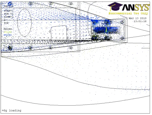
the grommet holes were drilled, an ANSYS stress vector plot was generated to show the stress
paths due to a +6g wing loading. Figure 2.4 shows the stress vector plot of the bottom left corner of the main bulkhead when viewed from the front.
Figure 2.4: Stress vector plot of main bulkhead
This plot shows that the magnitude of the stress in the bottom corners of the main bulkhead is negligible when compared to the failure stresses of the bulkhead material. This allows the
holes to be drilled without any detrimental effects to the structural integrity of the bulkhead.
The largest difference in the designed versus built aircraft is in the total weight. The Solid-Works model had Plank weighing 40 lbs while the built aircraft weighs 50.3 lbs. The weight
difference has two main causes: added components and structural weight. The constructed
aircraft components such as the wings and fuselage came out heavier than those in the Solid-Works model. Epoxy and paint were the main culprits for the added weight to the individual
components. The second main cause of the overall heavier weight was added components. The
Plank contains approximately 100 ft of servo wire and 14 ft of 12 ga motor wire. The total wire
weight is not insignificant when compared to the total weight of the aircraft.
2.3
Electrical System
The electrical system on board Plank is comprised of two subsystems: propulsion and avionics.
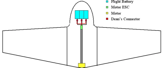
The propulsion power system is relatively simple in that its sole purpose is to supply the ESC (Electronic Speed Controller) and motor with power from the main flight batteries. Figure 2.5
shows the propulsion power system and its layout in the aircraft. The main flight batteries used
Figure 2.5: Propulsion power system
by Plank are three FlightPower 5000 mAh 10S lithium polymer batteries connected in parallel.
These feed into a Castle Creations 110 HV speed controller, which is bolted onto the bottom of the battery box extending into the flow coming through the cooling duct. The motor leads
from the speed controller run the length of the fuselage back to the AXI 5330/18 brushless
motor. The motor speed controller combination can handle at most 110 amps for no longer than 20 seconds and supply approximately 4000 Watts of power max. A measurement of the
continuous power for the static thrust case was made using a Wattmeter where the maximum
current was found to be around 65 amps, which corresponds to about 2400 Watts of power. The avionics subsystem provides power to all non-propulsion related electronics through
two 4500 mAh 6.0 Volt NiMH battery packs in parallel. These are located on both sides of
the battery box and feed into the receiver. Figure 2.6 shows a diagram of the avionics power system for the entire aircraft. The receiver powers nine JR DS8717 servos which are used to
actuate the control surfaces and for ground steering. Four servos are located in each wing and
Figure 2.6: Avionics power system
2.4
Brake System
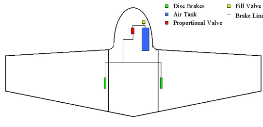
Plank was outfitted with a pneumatic braking system to decrease the stopping distance for
landings at Perkins field. The braking system used is manufactured by Robart and consists of a 43 in3 air tank feeding two pneumatic disc brakes located on the main gear, through a
proportional valve that is set to activate when a down elevator input is given. The air tank is charged to an initial pressure of 100 psi before flight. A leak test was performed on the brake
system and was shown to lose approximately 1 psi/hr. Figure 2.7 shows a layout of the braking
system.
Figure 2.7: Braking system
2.5
Flight Control Surfaces and Actuators
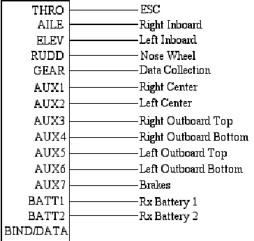
Plank contains a total of eight control surfaces with four on each wing. The inboard and center
control surfaces on each wing have been coupled together to function as elevons. This was done
function only as clamshell style drag rudders. The original design called for these surfaces to
provide elevator and aileron inputs as well, however, it was determined during the setup of the radio that this would require more mixers than the radio had available. The sizes and
deflections of each of the control surfaces can be found in the aircraft data sheet in Appendix
A. The final mapping for the control surfaces to the receiver along with all other servos is shown in Figure 2.8.
Figure 2.8: Servo mapping
2.6
Payload/Instrumentation
Plank was mainly designed around the momentum wheel stability augmentation system and
therefore, has a large amount of payload room. During the initial flights, the aircraft will be
flown without the momentum wheel or its supporting equipment. The payload on the initial flights will consist only of the Hazard IMU and EagleTree data logging system so that essential
aircraft parameters, such as airspeed and altitude, can be read in real time on the ground. Subsequent flights will be flown with dummy masses to ensure that Plank can handle the
additional loads before flying with the actual payload items. The payload items designed to
be carried by Plank include the momentum wheel, EagleTree, Hazard IMU, and the ASROV (Avionics System for Remotely Operated Vehicles) computer system.
One of the goals during the flight testing phase of Plank is to perform parameter
accel-erations and control surface positions. The Hazard IMU contains all of the necessary sensors
to gather the required data. Data is sampled at 50 Hz and stored on board in flash memory for download over USB after the flight. It is located in the nose of aircraft and is oriented such
that the accelerometers and gyroscopes are aligned with the principal axes of the aircraft. The
airspeed and altitude data is obtained from a pitot-static tube located just off the right side of the nose of the aircraft and extends forward approximately two feet. The control surface
posi-tions are determined indirectly from the PWM (Pulse Width Modulation) signal commanded
Chapter 3
Experiments/Results
3.1
Static Wing Load Test
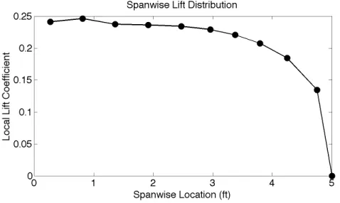
The purpose of the static wing load test was to show that the wings of Plank would be able to withstand the designed maximum safe loading of±6g’s. The load distribution on the wings was
determined from the spanwise lift distribution based on the AVL model of Plank. Figure 3.1
shows the lift distribution for Plank at the corner velocity of 87 ft/s in trimmed flight. The wing
Figure 3.1: Lift distribution across semi span
was divided into eight panels on which weight was placed to simulate the g loading. Figure 3.2 shows the panel distribution and Table 3.1 shows the width of each panel. Using the lift
distribution from Figure 3.1 and the panel layout from Table 3.1, the weight on each panel
for the test g loading was determined. Table 3.2 shows the applied weights at each location for each g load. To monitor the wing during the load test, a total of eight strain gages were
Figure 3.2: Panel layout for weight distribution
Table 3.1: Wing panel widths
Panel 1 2 3 4 5 6 7 8
Width (in) 6.67 6.66 6.68 4.98 5.09 4.97 6.03 5.98
Table 3.2: Weight distribution for simulated g loading (lbs)
g Load Panel
1 2 3 4 5 6 7 8 Total
bottom skin. Strain gage placement was based on the strain plots generated by ANSYS in
Figure 3.3 and Figure 3.4. The gages were placed in areas that had low stress gradients and
Figure 3.3: Strain plot for +6 g load, top skin
were free from stress concentrations [10]. Since the compressive strength of fiberglass is much lower than the tensile strength, the strain gages were used to monitor the compressive strain
on the wing instead of tensile strain. A conservative estimate for the compressive failure of the
wing skins of Plank was set at 18,000 psi. This was set based on data for the material properties of fiberglass from the database at http://www.matweb.com/. Figure 3.3 and Figure 3.4 show
that the maximum strain encountered in tension during the±6g load correlates to a stress value
of ≈11,600 psi. The maximum compressive strain encountered equates to ≈5900 psi. This is significantly lower than the 18,000 psi estimated failure and yields a safety factor of just over
three. The area of greatest stress and strain for both ±6g loads occurs where the wing joiner
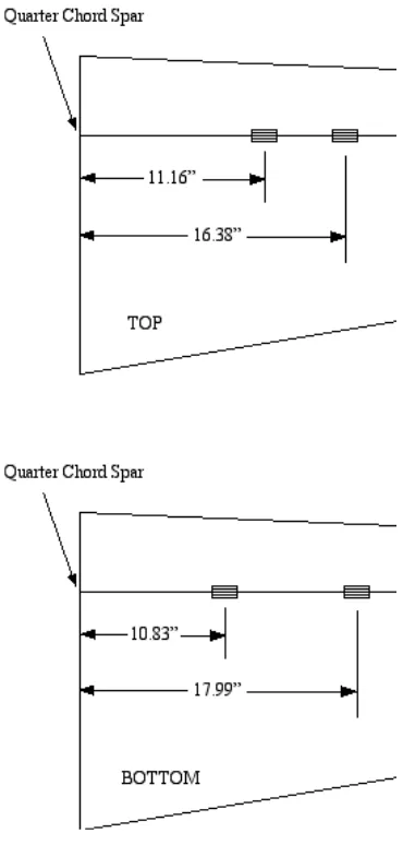
box ends at 6.25 inches from the root along the quarter chord spar and decreases towards the wing tip. For the +6g load in Figure 3.3, a lower strain gradient occurs in the area shown
between 705 and 1060 micro strain. Further analysis in this area indicated that the strain gage
was best placed directly above the spar at 11.16 inches from the root. Moving further outboard, another gage was placed at 16.38 inches. For the -6g load case in Figure 3.4, the same approach
was used and the strain gage locations were determined to be directly underneath the spar at
10.83 inches and the second at 18.00 inches. Figure 3.5 shows the locations where the strain gages were placed and Table 3.3 shows the numbering of the strain gages that was used in post
Figure 3.4: Strain plot for -6 g load, bottom skin
Table 3.3: Strain gage numbering
Strain Gage Location
1 Right Wing Top Inboard 2 Right Wing Top Outboard 3 Right Wing Bottom Inboard 4 Right Wing Bottom Outboard 5 Left Wing Top Inboard
Table 3.4: Predicted readings for strain gages during positive g loading (micro strain)
+g Loading Gage 1 & 5 Gage 2 & 6 Gage 3 & 7 Gage 4 & 8
1 -147 -95 314 274
2 -294 -190 627 549
3 -441 -265 941 823
4 -588 -379 1250 1100
5 -735 -474 1570 1370
6 -882 -569 1880 1650
Table 3.5: Predicted readings for strain gages during negative g loading (micro strain)
-g Loading Gage 1 & 5 Gage 2 & 6 Gage 3 & 7 Gage 4 & 8
1 289 190 -143 -83
2 559 479 -286 -167
3 868 768 -429 -249
4 1117 957 -572 -332
5 1412 1180 -715 -416
6 1675 1436 -858 -500
During the wing load test the strain gage readings were monitored to ensure the wing behaved as expected and that the maximum strain values were not exceeded. The expected
strain readings given by ANSYS for each of the strain gage locations can be found in Table 3.4
and Table 3.5.
3.1.1 Equipment 1. Plank UAV
2. Plank bottom and top fuselage molds
3. 242 lbs of lead shot
4. Strain gage kit
5. Eight strain gages
7. Strain gage reading equipment
8. Ruler
9. Non-slip drawer liner
10. Soldering equipment
3.1.2 Procedure
The areas where the strain gages were bonded were prepared using 400 grit sand paper and surface cleaner. The strain gages were then bonded to the locations specified in Figure 3.5 using
the bonding procedures provided by the manufacturer. Wire was soldered to the strain gages
and a strain relief added to prevent the gages from being torn off during handling. The fuselage molds were placed on the ground facing each other, which allowed Plank to be easily moved
from one mold half to the other, and prevented weights from falling long distances and injuring
personnel during testing. Using a sharpie, the panel layout was marked off on the non-slip liner and applied to the wing. The strain gage wires were connected to the computer interface
and calibrated according to the software’s procedure. Using a ruler, the distance between the
ground and each wing tip was recorded as the initial zero position. The 1g load case was applied by placing the appropriate amount of weight on each wing panel. The weight was placed from
the root outwards on both wings at once. This procedure was used whenever weight was added to the wing. Weight was removed in the opposite manner. Once the strain readings on the
computer leveled out, the wing tip deflections were measured and the next load case applied.
During the wing load test, all those involved were instructed to listen for any creaks coming form the wings so that catastrophic failure could be prevented.
3.1.3 Results
The wings for Plank were successfully able to withstand the ±6g load without failure or per-manent deformation. It was noted during the test that the wing tip deflections exceeded their
predicted values and the gap between the wing and fuselage joint expanded during loading.
These observations correlate well with the behaviors visible in the reduced data. Figure 3.6 through 3.9 shows the strain as a function of g loading for each loading case and wing.
The ANSYS predicted strain values did not match with the actual strain values recorded.
For each loading case, the strain gages in compression matched more closely with the predicted values than the strain gages in tension. This discrepancy has two main causes: the estimation
of the modulus of elasticity and the constraints at the wing root. The modulus of elasticity was
Figure 3.6: Strain vs negative g loading for left wing
Figure 3.7: Strain vs negative g loading for right wing
Figure 3.9: Strain vs positive g loading for right wing
in ANSYS. The second cause for the discrepancy in the data is believed to have contributed
more to the difference then the estimation of the modulus of elasticity. The ANSYS model has
the spar joiner box fixed to the spar and main bulkhead, while inside Plank the joiner box has 10 bolts that mount the box to the bulkhead. During the wing load test, it was evident that this
joiner box was rotating, which caused the wing fuselage gap on the tension side to increase in
size and on the compression side to decrease. Before the wing load test was conducted, a piece of masking tape was placed underneath the wing joiner box to show any movement of the joiner
box. A post test inspection of the aircraft revealed that the joiner boxes had displaced the tape
indicating rotation. This rotation increased as the loading increased on the wing, causing the gap between the wing and fuselage to increase in size, which ultimately led to greater than
expected wing tip deflection as shown in Figure 3.10 and Figure 3.11. The joiner box rotation
Figure 3.11: Wing tip deflection under positive g loading
was also evident in the residual wing tip deflection shown in Figure 3.12 and Figure 3.13.
Figure 3.12: Residual wing tip deflection after negative g loading
As stated earlier, the joiner box rotation caused the wing fuselage gap on the compression side to close, causing the skins to touch and provide a load path. This matched closely with
the constraints set up in ANSYS and therefore, matched the recorded data relatively well as
seen in Figure 3.6 through 3.9. On the tension side of the wing, the gap removed the load path which caused the skin to exhibit lower strain since it was no longer constrained in the spanwise
direction.
The continuous loading and unloading of the wings through flight testing will eventually cause the joiner box to widen the bolt holes in the main bulkhead. To fully constrain the joiner
Figure 3.13: Residual wing tip deflection after positive g loading
Table 3.6: CG location vs aircraft configuration
Aircraft Configuration CG Location (in)*
Wing and Half Tail (0.75ft) 5.59 - need new value for CMARC Wing and Full Tail (1.5ft) 5.99
*Measured from the leading edge of the wing/fuselage joint
3.2
Center of Gravity/Moments of Inertia
The center of gravity (CG) and moment of inertia test was conducted to set the CG of the
aircraft at the required location and to determine the moments of inertia about the aircraft’s
body axis for use in stability and control and performance calculations.
The CG of Plank was determined through a method that required the aircraft to be
sus-pended from a beam using a single pivot point. This followed that a vertical line dropped from
the point of suspension would intersect the CG of the aircraft. Suspending the aircraft at two different angles yielded the vertical and longitudinal CG locations [6]. The longitudinal CG
of Plank was predetermined based on stability requirements and has a set location. The CG
locations for the full and half tail configurations can be found in Table 3.6.
These CG locations provided a 10% static margin for each configuration. When the aircraft
was balanced about the required CG location, the fuselage hung level with the ground. This simplified the determination of the vertical CG since the vertical CG in this case lay directly
below the longitudinal CG location. Suspending the aircraft from a second point created a
Figure 3.14: Vertical CG Geometry
Table 3.7: Values of Dfor each configuration
Aircraft Configuration Est. Vertical CG (in)* Value ofD(in)**
Wing and Half Tail (0.75ft) -0.96 2.18 Wing and Full Tail (1.5ft) -0.96 2.18 *Measured from the leading edge of the wing/fuselage joint
**Measured from the required longitudinal CG location for each configuration
the aircraft is suspended at is θ. If θ is small, than 90−θ will be large and any errors in the
measurement ofθwill cause a large shift in the vertical CG. To minimize errors,θshould be as
large as practically possible. Using the distance D and the angle θ, the distance between the hole and the vertical CG was determined using the following equation
x=Dtan(90−θ) (3.1)
Equation 3.1 contains two unknown variables: x and D. The value for Dwas estimated using
the SolidWorks model of Plank. The SolidWorks model was configured to mirror each aircraft
configuration and give an estimate of the location of the vertical CG. Table 3.7 contains the estimated vertical CG locations and the values of D for each configuration that should allow
the plane to hang at a 30◦ angle.
holes marked.
Figure 3.15: CG/MOI plates for Plank
The moments of inertia of Plank were determined through a method that swings the aircraft
like a pendulum and uses the oscillation data, apparatus geometry, and aircraft geometry to
back out the moments of inertia about thex,y, andzaxes. To measure the moment of inertia of a single axis, the aircraft was suspended so the axis of rotation was parallel with or coincident
to the axis that the moment of inertia was obtained for [6]. The swinging rig added to the total
moment of inertia of the aircraft so it must be subtracted out from each axis. Also the aircraft was not being oscillated about its own axes and therefore the moment of inertia was transferred
to it using the parallel axis theorem. Whenever an oscillation was induced on the aircraft, it was kept as small as practical. The equations used to calculate the moments of inertia of the
aircraft are based on small angle approximations and therefore the magnitude of the oscillations
was kept small so as not to violate the small angle approximation.
Since the aircraft was suspended by the CG/MOI plates, the total moment of inertia was
greater than that with the plates removed. However, it was shown that the moments of inertia
of the plates were negligible when compared to the total moments of inertia of the aircraft. The moments of inertia of the CG/MOI plates about the CG of the aircraft were calculated using
the parallel axis theorem where
Ic=Icm+mr2 (3.2)
In equation 3.2Icis the moment of inertia about an axisc,Icm is the moment of inertia of the plate about its centroid, m is the mass, and r is the perpendicular distance between the two axes. The moments of inertia of the plate about its centroid, without cutouts, are given by the
equations
Ix=
m(b2+c2)
Table 3.8: Estimated moments of inertia of Plank and CG/MOI plates
Configuration Moment of Inertia
Plank (slug−f t2)
CG/MOI Plates (slug−f t2)
% of Total
Wing and Half Tail (0.75ft)
Ix 4.124 0.032 0.26
Iy 3.309 0.005 0.16
Iz 7.127 0.035 0.15
Wing and Full Tail (1.5ft)
Ix 4.124 0.60
Iy 3.608 0.49
Iz 7.426 0.48
Iy =
m(a2+b2)
12 (3.4)
Iz =
m(a2+c2)
12 (3.5)
where
• a= the length of the plate along the x axis
• b= the length along the zaxis
• c= the length along the y axis.
Using equations 3.2 through 3.5 the moments of inertia of the plates were determined and
can be found in Table 3.8 along with the estimated moments of inertia of Plank about its CG for each configuration. The CG/MOI plates were shown to contribute less than 1% to the total
moments of inertia of the aircraft and were therefore considered to be negligible.
The moments of inertia about all three axes cannot be obtained through the use of a single pendulum. Two types of pendulums were required, a compound pendulum to measure the
moments of inertia about thex andy axes, and a bifilar pendulum to measure the moments of
inertia about thezaxis [6]. Since the CG/MOI plates were found to be negligible, the equations used to calculate the moments of inertia about the x,y, and z axes were modified to exclude
the terms that dealt with the swinging rig alone. The equation used to calculate the moment
of inertia about the xand y axis was
Ic=
W T2L
4π2 −
W L2
where
• Ic =Ix orIy depending on the orientation of the aircraft
• W = weight of the aircraft
• T = period of aircraft
• L= distance from axis of rotation to CG of the aircraft
For the bifilar pendulum, the equation used to calculate the moment of inertia about the z
axis was
Iz =
W T2A2
16π2L (3.7)
whereLis the length of the vertical suspension lines andAis the distance between the vertical
lines.
When using the compound pendulum, the length of the ropes suspending the aircraft were
kept as short as possible so that the aircrafts moment of inertia about the measuring axis would be a large percent of the total moment of inertia. For the bifilar pendulum, the vertical
ropes suspending the compound pendulum were equal to or greater in length than the distance
between them for the same reason [6].
3.2.1 Equipment
The equipment used to determine the center of gravity and moments of inertia of Plank consisted
of the following items.
1. Plank
2. Two CG/MOI plates installed on Plank
3. Two stands
4. Rectangular aluminum suspension beam
5. Rope
6. Two stopwatches
7. Inclinometer
8. Aluminum tube
The stands were setup to support the steel beam from which the aircraft was suspended.
The distance between the stands varied depending on the aircraft configuration being tested, but were kept as close together as possible to minimize beam flexing. For the CG test the rope
was suspended from the beam at a single point and both ends attached to the CG/MOI plates
on Planks wings. Figure 3.16 shows the set up used to measure the CG.
Figure 3.16: Plank in CG configuration
For the moment of inertia tests about the xand y axes, the compound pendulum was used
where the aircraft was suspended from the beam by two points with the ropes attached at both ends of the CG/MOI plates. Figure 3.17 and Figure 3.18 show the setup that was used for
measuring the moments of inertia about thex and y axis respectively. Measuring the moment
of inertia about the z axis required the use of the bifilar pendulum. The setup used for this test is shown in Figure 3.19.
3.2.2 Procedure
Before any testing was conducted, the aircraft weight was obtained, as it was necessary for all
subsequent calculations. The CG/MOI plates were balanced prior to installation so that they did not affect the CG of the aircraft. The CG setting was completed before moment of inertia
testing, as it was required in the calculations for the moments of inertia. The test rig was setup according to Figure 3.16 with the vertical tails located 1.5 ft behind the trailing edge of the
wing and the aircraft suspended from the point on the CG/MOI plates that corresponded to
Figure 3.17: Plank in the configuration for measuringIx
Table 3.9: Vertical CG of Plank
Configuration θ (deg) D(in) VCG (in)*
Full Tail 31.1 2.18 3.61 Half Tail 30.9 2.18 3.64
*Measured from the longitudinal CG hole on the CG/MOI plate
as a guide, the internal payload was shifted until the top of the CG/MOI plates were level with the ground. Additional mass was required to set the longitudinal CG at the required location.
Once the longitudinal CG had been set, the rope attached to the CG/MOI plates was moved to the hole with the appropriate VCG label. The inclinometer was used to determine the angle of
suspension and through equation 3.1, the vertical CG was found. This procedure was repeated
for the tail located 0.75 ft behind the trailing edge of the wing.
The moment of inertia about the x axis was determined first using the setup as shown
in Figure 3.17 with the tail located 1.5 ft behind the trailing edge of the wing. The aircraft
was rotated to approximately 15◦ along the axis of rotation and released. Two observes used stopwatches to determine the time of ten oscillations. The strings were lengthened by two inches
and the process was repeated. This procedure was repeated for the half tail configuration. The
same procedure was used to determine the moment of inertia about they axis, using the setup as shown in Figure 3.18.
The moment of inertia about thezaxis required the pendulum to be modified and setup in
the bifilar configuration according to Figure 3.19. Again the aircraft was rotated approximately 15◦ about the z axis and released. The oscillation data and length of rope were recorded and the procedure repeated for the half tail configuration.
3.2.3 Results
The center of gravity of Plank for each configuration was setup using the CG information from
Table 3.6. Lead weights were placed in the nose of the aircraft until the inclinometer read 0.0◦. The vertical CG was then determined through the specified method with the results found in Table 3.9. The data gathered from the moments of inertia testing was processed in an excel
spreadsheet with the average moment of inertia for each axis given in Table 3.10. The
Solid-Works estimated moments of inertia were less than the measured moments of inertia for every axis and configuration. As mentioned in section 2.2, the SolidWorks model did not contain any
wire, mounting shelves, mounting hardware, or brake lines. The addition of these components
Table 3.10: Estimated and measured moments of inertia
Configuration Axis SolidWorks Estimated Moments of Inertia (slugf t2)
Measured Moments of Inertia (slugf t2)
Half Tail x 4.124 5.608
y 3.309 3.924
z 7.127 7.505
Full Tail x 4.124 5.412
y 3.608 3.814
z 7.426 8.329
as evident by the difference in designed vs measured in Table 3.10. These updated moments of inertia have been incorporated into the performance calculations and the stability and control
code to provide more accurate results.
3.3
Drop Test
The purpose of the drop test is to ensure that Plank can withstand the vertical velocities
associated with a hard landing. The landing gear was tested to a vertical velocity of 10 ft/s,
which is a requirement outlined by the Joint Services Specifications Guide 2009 for aircraft landing on solid ground [8]. The landing gear was tested individually so the experimental
parameters could be closely controlled and to reduce the overall weight used in the experiment.
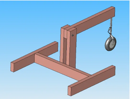
The apparatus utilized a lever design that allowed the gear to impact the ground in a controlled and repeatable manner. Figure 3.20 shows a diagram of apparatus. Since the lever rotates about
a pivot point, the tangential velocity at impact must be 10 ft/s. The angle that the lever arm must be rotated to can be determined through the equations
Vf2=Vi2+ 2g∆h (3.8)
θ=sin−1(∆h
r ) (3.9)
For a lever arm that is 2 ft in length, it must be rotated to an angle of 51.0◦ to attain the required impact velocity. For this test the landing gear was loaded with a reduced weight to simulate wing lift during landing. The testing weight was determined so that the impact energy
Figure 3.20: Landing gear testing apparatus
[7]. The equation used to determined the reduced testing weight was
WT r =WT e VV2
2g + (1 +KL)d V2
V
2g +d
(3.10)
where
• WT r = reduced weight that the aircraft will be tested at
• WT e = weight of the equivalent air-borne impact
• VV = vertical velocity
• g = acceleration of gravity
• KL = lift factor (L/WT e)
• d= mass travel from time of ground contact
The lift factor used to determine the reduced drop weight was 0.5, which yields a reduced
dropping weight of 51.1 lbs for a 52.5 lb aircraft. The value of d used in equation 3.10 is the compression stroke of the Robart 682 strut, which is 1.06 inches. The weight distribution
on the landing gear determined how much energy each strut had to absorb and varied with
Table 3.11: Landing gear weight distribution
CG = (need value) Distance from CG (in) Supporting Weight (lbs) % of Total Weight
Nose Gear 21.59 6.52 12.8
Main Gear 3.16 44.56 87.2
*Measured from leading edge of wing/fuselage joint
farthest aft CG, and therefore had the highest percentage of weight on the main gears. In this configuration the weight on the landing gear was found through the equations
WT r=Wn+Wm (3.11)
0 =Wnxn−Wmxm (3.12)
where
• Wn = weight on the nose gear
• Wm = weight on the main gear
• xn = distance from the CG to the nose gear
• xm = distance from the CG to the main gear
Table 3.11 contains the calculated weight distribution and values used in equations 3.11 and 3.12. For this test each main gear was loaded with 22.28 lbs. The goal of this drop test was
to have each strut reach maximum stroke when impacted at 10 ft/s. Since the energy of the drop must be absorbed in a short stroke, the strut requires a high spring constant and high
damping value. The springs provided with the Robart struts were stated to be adequate for
planes up to 50 lbs. However, upon installation it was noticed that the springs were not stiff enough to prevent partial strut compression under the aircraft’s weight. Sorbothane was used
to increase the overall spring constant of the landing gear and provide damping. The process for
determining the amount of Sorbothane necessary to provide adequate spring force and damping was trial and error. To minimize damage to the aircraft during this process, the testing rig was
used to tune the landing gear springs before dropping the actual aircraft. A measuring device
placed on the landing gear strut allowed the compression stroke distance to be measured using a high-speed camera. The measuring device consisted of black and white rectangles 0.25 inches
Figure 3.21: Measurement of strut deflection
3.3.1 Equipment
The apparatus used to conduct the drop test consisted of the following items:
• Two Stands
• Rectangular aluminum suspension beam
• CG/MOI Plates
• Plank
• Rope
• High-speed camera and necessary equipment
• Lights
• Ruler
• Pulley
• Drop test rig
• Weights
• Scale
3.3.2 Procedure
The landing gear was mounted to the test rig and setup with the proper amount of weight
using the weights and scale. The high-speed camera and necessary lighting were placed so that
the bottom half of the strut was visible when the gear was resting on the ground. The testing area was cleared and the drop arm raised to the required angle using the inclinometer. The
high-speed camera was set to record and the drop arm released. The landing gear was
visu-ally inspected for damage after each drop. The high-speed video footage was then analyzed to determine the strut compression during the fall and to verify impact velocity. If the struts
bot-tomed out early, the landing gear was disassembled and Sorbothane added. This was repeated
until the landing gear behaved as desired. Once the landing gear had been tuned, they were reinstalled on Plank along with the CG/MOI plates. The high-speed camera was repositioned
so that all struts were visible while the aircraft was on the ground. The drop procedure was repeated with the aircraft suspended at a 5◦ nose up angle to simulate a landing flare. The aircraft was dropped four times starting at 25% total drop height and increased by 25% each
time until dropped from 18.5 inches. In addition to inspecting all components of the landing gear and mounts, the internal aircraft structures, payloads, and wing joiners were also inspected
after each drop.
3.3.3 Results
The testing and tuning of the individual landing gear as well as the full aircraft drop were completed successfully. Each gear was tested individually at a 10 ft/s drop velocity with a
reduced weight to compensate for wing lift during landing. The only modification made to the
main landing gear was the addition of Sorbothane. One strip of Sorbothane 0.5 x 0.25 x 10 inches was inserted in to the center of the spring. The original pre-compression was left in the
spring. This modification was made to both main landing gear and each behaved as desired
during drop testing, compressing the strut 75% of the total distance. Figure 3.22a shows the main gear at maximum compression during the individual drop test. The nose gear required
more modification than the mains to behave as desired. The spring was shortened by 2.5 inches and a strip of Sorbothane, with dimensions 0.5 x 0.25 x 7.5 inches, was placed in the center
of the spring. Also, the pre-compression was reduced from 2 inches to 1 inch. The drop test
showed the nose gear compressed 90% of the total stroke distance. Figure 3.22b shows the nose gear at maximum compression.
With each landing gear tuned, they were re-installed on Plank, aircraft weight set for the
correct reduced dropping weight, and CG set. The aft most tail configuration was the only configuration that was drop tested since it produced the greatest moment on the boom fuselage
(a) Main landing gear at maxi-mum compression
(b) Nose gear at maximum com-pression
drop, the aircraft was suspended by rope and the rope cut to release the aircraft since any
pulley system would cause the stands holding the suspension beam to tip over. The cutting of the string proved to be unsafe, since personnel had to stand near the aircraft, and required time
to tie a new string after each drop. To remedy the problem, the trigger mechanism used on
the standard NCSU launcher was installed vertically on the suspension beam which allowed for the aircraft to be easily and quickly repositioned after a drop and allowed the person initiating
the drop to remain clear of the aircraft. Four drops were conducted with the main gear height
being 25, 50, 75, and 100% of the drop height. During the first drop at 4.63 inches (25%), the front hatch was not properly secured and the hardpoint located at the rear of the hatch came
off. This was the only damage noted during this drop. The second drop at 9.25 inches (50%)
showed no damage to the aircraft. During the third drop from 13.9 inches (75%), the magnetic hatches from underneath each wing came off. The wing hatches were left off for the final drop.
The final drop from 18.5 inches showed no physical damage to the aircraft. However, the bolts
holding the landing gear mounts to the fuselage rib showed evidence of movement. The washers used on all of these bolts were originally centered on the bolts, but after the drop each bolt had
moved to the top of the washer and scratch marks on the washers indicate upward movement
of the bolts. The rib that the landing gear mount was attached to was inspected for damage from the traveling bolts but none was found.
3.4
Motor Mount Test
The purpose of this test was to ensure that the motor bulkhead that the propulsion system for
Plank is mounted to, can withstand the maximum expected flight loads. This test addressed
one of the catastrophic failure modes outlined by SLAT (System Level Airworthiness Tool) that could occur with the propulsion system. SLAT is a systems engineering framework designed to
help determine requirements for fixed wing UAS flights over populated regions [2]. A further
discussion of SLAT and overall system safety can be found in Chapter 6.
As previously discussed, the propulsion system for Plank is comprised of an AXI 5330/18
electric brushless motor turning a 17x8 four bladed propeller. Based on previously completed
wind tunnel tests, the motor propeller combination is estimated to yield a maximum thrust of 16 lbs and 2 ft-lbs of torque [1]. During the wind tunnel tests the motor was never run up to
100% throttle due to vibration limitations, therefore, the motor bulkhead was tested to 150% of
the maximum expected loads. This ensured that the bulkhead could withstand the estimated maximum loading and any variations due to error.
The bulkhead testing was conducted with a setup that used stand off mounts to which the motor thrust and torque were applied. The simulated motor torque was applied through a
furthest hole from the center, which corresponded to a moment arm of 9 inches, and required
a 4 lb weight to achieve 150% of the maximum expected torque load.
Figure 3.23: Setup used to apply torque load
The thrust setup was more difficult as it required the force to be applied along the aircrafts
thrust line. This was accomplished with a moment arm to which weights were applied to
simulate the thrust force. Figure 3.24 shows a diagram of the setup where W is a hanging weight and F is the force applied by the hanging weight. Based on the setup, the moment
applied byW is
MW =LW cos(45◦) (3.13)
and the moment seen byF is
MF =LF sin(45◦) (3.14)
Setting the moments equal shows that
MW =MF
LW cos(45◦) =LF sin(45◦) (3.15)
W =F
A 24 lb weight was required to achieve 150% of the estimated maximum thrust load. The
force was applied using the setup shown in Figure 3.25. The front portion of the test rig (bottom
Figure 3.24: Diagram of thrust setup
3.4.1 Equipment
The equipment used to conduct the motor bulkhead testing consisted of the following items:
• Plank
• Motor simulator
• Torque bar
• Weights
• Thrust rig
• Inclinometer
3.4.2 Procedure
Testing was conducted in two phases, torque testing and thrust testing. The AXI brushless
motor was removed from Plank and the motor simulator and torque bar installed on to the motor bulkhead as seen in Figure 3.23. The 4 lb weight was attached to the last hole on the
left side of the torque bar. The weight was removed and the bulkhead inspected for damage.
The weight was then attached to the last hole on the right side of the torque bar. Again the bulkhead was inspected upon weight removal. The torque bar was then removed and replaced
with the thrust rig. Using the inclinometer, the arm was placed at a 45◦ angle when resting on the motor simulator with the 24 lb weight applied. The weight was removed and the bulkhead inspected for damage.
3.4.3 Results
The motor mount was successfully able to withstand 150% of the estimated maximum thrust and torque loads. No cracking was heard during the testing and a post test inspection showed
no signs of deformation or damage.
3.5
Control Surface Calibration
The purpose of the control surface calibration was to set the deflection angles for each control
surface of Plank and determine the PWM signal associated with each deflection. The required deflections for each control surface can be found in Table 3.12. The control surface deflections
were set using a laser and a mirror mounted to the control surface. The laser beam was reflected
Table 3.12: Control surface deflections
Control Surface Deflection Range for Low Rates
(deg)
Deflection Range for Standard
Rates (deg)
Deflection Range for High Rates
(deg)
Inboard Elevon ±15 ±20 ±25
Center Elevon ±15 ±20 ±25
Top Drag Rudder 0 to -20 0 to -30 0 to -40 Bottom Drag Rudder 0 to +20 0 to +30 0 to +40
surface deflection. Figure 3.26 shows the geometry of the setup. Based on the geometry of the
Figure 3.26: Mirror laster geometry
setup, the angle that the deflected laser beam creates with the horizontal is twice that of the
deflection of the control surface. Since the beam was reflected onto a horizontal surface, the deflection of the control surface in degrees was determined using the equation
D= tan
−1(H L)
The second portion of this experiment dealt with the PWM signal from the receiver. This
signal was recorded in order to generate a calibration curve so that a PWM signal from the receiver can be mapped to a control surface deflection angle.
3.5.1 Measurement Error
Large portions of measurement error associated with the laser-mirror setup are due to the
dis-tances used in the setup. As the distance between the mirror and wall increases, the horizontal distance seen on the wall during deflection also increases. This provides greater accuracy for
each degree of deflection. The distance between the wall and mirror was the most difficult distance to measure accurately and therefore, was subject to the greatest amount of error. The
apparatus setup used a distance of 10 ft between the mirror and wall. Assuming that this
distance was measured to±0.5 inches, the measured angle fell within±0.06◦ of the true value. This was found by adding or subtracting 0.5 inches to the variableL in equation 3.16 and
cal-culating the value forH. This value was then converted back to a deflection angle assuming no
error in the measurement between the wall and the mirror. The error bounds of the deflection angle change with the angle and range from±0.02 to±0.06◦.
3.5.2 Equipment
The equipment used to conduct the control surface calibration consisted of the following items:
• Left and Right wings of Plank
• Laser
• Mirror
• Tape
• Marker
• Wall
• Transmitter
• Receiver
• Receiver battery
• Tape measure
Figure 3.27: Control surface calibration setup
The setup that was used to conduct the calibration is shown in Figure 3.27. The wing was
setup so that the mirror was mounted as close the hinge line as possible without binding and
with the hinge line being vertical. The laser was placed so the beam reflected horizontally when there was zero deflection on the control surface.
3.5.3 Procedure
Testing was conducted in two phases: setting of deflection angles and calibration through PWM
capture. In phase one, the equipment was setup according to Figure 3.27. The servos were connected to the receiver and then both transmitter and receiver powered up. The laser was
setup so the beam reflected horizontally onto the wall. Using the tape measure, the distance
from the wall to the mirror was measured and adjusted as necessary. Using equation 3.16, the horizontal distances on the wall that correspond to the desired deflection angles for high
rates were marked out. The surface was deflected until the laser beam reached the specified horizontal distance. If adjustments were needed to the servo travel, large adjustments were
made by changing the linkage geometry, while small adjustments were made by using the end
point adjustment feature in the transmitter. This was repeated for all control surfaces on each wing. For the low and standard rates, the dual rates function was utilized in the transmitter.
For standard rates the dual rates function was adjusted to±80% and±60% for low rates.
The data logger was connected to the elevator, aileron, and the appropriate auxiliary channel
for the drag rudder of the wing being tested. Using equation 3.16, 2.5◦ increments were marked out on the wall up to the maximum deflection angle seen in high rates. All control surfaces were
centered and data logger set to record. The elevator was moved up 2.5◦ and held there for five seconds. This process was repeated in 2.5◦ increments up to the maximum deflection angle for the elevator. The above process was repeated for all control surfaces in both directions of travel
where applicable. The data logger was then stopped and data retrieved using a computer.
3.5.4 Results
The control surface deflection angles for each rate were setup successfully and the PWM signal
for each deflection captured. The dual rates for each surface were set up on their respective
switches on the transmitter with the switch ”0” position being high rates, ”1” position mid rates, and ”2” position low rates. The PWM signal was captured in high rates to span the
full range of each control surface. Plots of the PWM signal versus deflection angle for each
control surface can be found in Figure 3.28a through 3.28f. These plots will be used to analyze post flight data on control surface movement. The Hazard IMU logs the PWM signals from
the servos, which can be converted to a deflection angle using the calibration plots. A Gauss interpolation will be used for PWM values that fall between the recorded data points.
3.6
Taxi Testing
To ensure that the aircraft’s ground handling characteristics are satisfactory, a low speed and
high speed taxi test were conducted. The taxi tests took place at Harnett County Regional
Airport (KHRJ) because the large open paved areas decreased the risk of damage to the aircraft due to various possible failures. The low speed taxi test was conducted first and tested the
aircraft’s tracking and turning radius. This was all completed on the tarmac and taxiway. The
high speed taxi test was conducted on the runway and tested the aircraft’s ground handling at speeds less than Vstall and for use in comparison with the take-off code and performance analysis.
3.6.1 Equipment • Plank
• Flight and avionics batteries for Plank
• Transmitter
(a) Left inboard elevon calibration (b) Left center elevon calibration
(c) Right inboard elevon calibration (d) Right center elevon calibration
(e) Left drag rudder calibration (f) Right drag rudder calibration
• Brake pump
• EagleTree
• Hazard IMU
3.6.2 Procedure
The procedure for the taxi test was done in two parts, one for low speed and one for high speed. For the low speed taxi test the aircraft was assembled on the tarmac according to the
standard operating procedures (SOP). The brakes were charged to 100 psi and the aircraft
transmitter switched into ”ground mode.” The aircraft was then given a push by hand and the brakes engaged by applying down elevator. This was performed several times at various speeds
to ensure the brakes were functioning properly and were not causing the wheels to lock up.
Tracking was tested next by placing the aircraft over the taxiway center line and ensuring all personnel clear of the plane of the propeller. The throttle was advanced until the aircraft
began to roll down the taxiway. Tracking was adjusted using the subtrim menu in transmitter
until the aircraft was able to track the centerline to the pilots satisfaction.
The turning radius for the aircraft was determined for each of the rates (high,standard,low)
by positioning the aircraft along the centerline of the taxiway, giving full rudder input, and
taxing until facing 180◦from its original position as seen in Figure 3.29. The tape measure was then used to measure the distance from where the aircraft started to where it stopped. The
test was conducted for each rate and the measured distance X recorded.
Once the tracking and brakes were adjusted based on the low speed taxi test, the aircraft was moved on to the runway for the high speed taxi test. It was decided that during the
taxi test the airspeed of Plank would be kept below 85% of the stall speed (31 mph) so that
rotation would not be achieved. The aircraft was placed on the runway center line and all personnel cleared from the runway. The throttle was advanced to full and the aircraft allowed
to accelerate. Airspeeds given by EagleTree were continually read allowed for the pilot. The velocity at which the throttle was brought back to zero was at the pilots discretion as the ground
handling at higher speeds was unknown. Tracking was adjusted until considered satisfactory
by the pilot at which point the final airspeed of each run was increased until just under the maximum allowable airspeed for the high speed taxi test.
3.6.3 Results
The low speed taxi test revealed that the brakes functioned well and did not need adjustment;
Figure 3.29: Turning radius test
the dual rates menu. This allowed the steering/tracking to be more easily controlled during taxi at high speeds. The turning radius for each rate was found using the method described
by Figure 3.29. Since the recorded distance X is the diameter of the semicircle, the distance was divided by two to obtain the turning radius which has been recorded for each rate in Table
3.13.
For the high speed taxi test, a total of seven runs were completed with the data given in Table 3.14. The acceleration data provided by the Hazard IMU was used to calculate the distance
the aircraft traveled during acceleration and the total time of acceleration. The duration of
Table 3.13: Turning radius
Rate Turning Radius (ft)
Low 21.50
Standard 7.00