Improvement of the Topology Optimization of Internally Ribbed Structure

(1)

Improvement of the Topology Optimization of Internally Ribbed Structure

Ryszard Kutylowski

Institute of Civil Engineering (I-14), Wroclaw University of Technology, Wroclaw, Poland

ABSTRACT

To make as safety as possible the nuclear power plants structures is the goal of the designers work. We realize that the structure is more safe when it is more stiff and what is equivalent it is less compliant, which means in case we try to find the most stiffer structure we should make the structure less compliant. From the other hand sometimes it is better when we make the structure less stiffer, but we are able to predict the behavior of the structure under the normally unexpected loading which can occurring during random failure (especially for example degraded core accident).

The main goal of this paper is to show the behavior of the structure when we change the stiffness of the structure by imposing more or less stiffer material into the sensitive structure design points. Using this procedure the structure becomes smart structure what is very needed in the safety considerations.

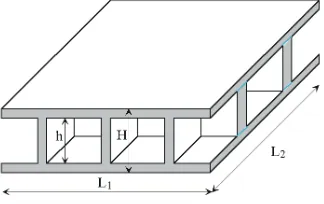
The strain energy is the equivalent of the mean compliance of the structure. Minimizing the mean compliance under the mass constraints we should solve the problem which means we are able to answer the question how to distribute the material within the design domain to obtain the most safe structure. The problem is solved in general, but it is illustrated using the internally ribbed structure (Fig. 1). This structure is very strong and it is useful to the most stressed structure elements. Additionally, using it and taking into account the hints proposed in this paper we can control the destruction process and we can avoid unexpected ruins of the structure.

INTRODUCTION

Presented problem is discussed from topology optimization point of view. Topology optimization answer the question of the topology of the structure (material distribution) within the design domain under the prescribed load and boundary conditions. This paper is generally based on SIMP method, but it was improved in[1], where the original, very fast topology optimization procedure was discussed from the strain energy point of view in aspect of the topology optimization steering parameters. The newest book summarized the latest achievements in the field of topology optimization was written by Bendsøe, Sigmund[2] in 2003. Because topology optimization is developing very rapidly in last decade, a lot of papers is publishing each year and they are showing new ways of the analysing and they are completing considered research field solutions and they are showing new applications in various field of activity.

The analysis when we change the material in chosen design point is presented in this paper. Follow this the designer may change the static scheme of the structure and may control the destruction process during the accident. The designer may choose the way of the destruction of the structure to make this process as safety as possible. In this case we are able to protect the most important parts of the structure, parts which cover the dispatch room or very important equipment or core for example. As a designers we know the risk dominant accidents and this is why we can predict or even decide how the structure can be have an accident. We should control the degradation process. To do that we should construct the structure in the proper way. In this paper the analysis of various structure models adequate to various possible static scheme (destruction models) will be done. This can answer the question how to construct the structure to be safe during unexpected destruction process. Additionally it is worth to mention, the topology of the structure will be optimal for each designed case. It will be indicated which cases are “less optimal”, but more safe. When the structure becomes less stiff, from the strain energy point of view it becomes less optimal, but what is more important we usually can control the behavior of this structure and we can predict the destructing process.

In[3] the problem of optimal placing ribs in the structure from Fig. 1 was discussed. Depends on the available amount of mass of the structure various ribs topology was obtained. The mass was made of one material.

Fig. 1. Internally ribbed plate

(2)

In this paper the previous solution is improved by imposing the stronger or weak material in the most stressed domains or in special chosen design points what can make the structure more safe. In the literature the topology optimization problems are considered for one material only what make not possible the discussion various destructing models of the structure.

This paper extend the topology optimization approach used to the internally ribbed structure into a new class of problem when the designer can model the destruction process. Theoretical formulation was properly extended and what is most important the procedures, which change considered simple structure to the smart structure were prepared. These procedures can be a part of the smart design process and they can be treated as a part of the “computer aids designer” system.

THEORY

In this research the variational approach is adopted to the situation when the designer wants to change the material in some design points. The mean compliance of the structure which is the objective function of the problem can be written as:

F( (x), ) C ( (x))eijekld ( hd m0)

l k j

i ₊

-=

_ò

W W W r l W r l

r (1)

where Cijkl is a

e

lasticity tensor, ris a density of material, rh is a density of homogenized material, l is a Lagrangre multiplier and m0 is an available mass. The constraints put on the mass of the structure is described by

( ) 1 0

0 = -= m m

H r_j j (2)

where m_j is a mass for j-th optimization step and it this case it is defined as

mj =mj_W_m +mj_Wv+mj_Ww_s (3)

where W_m is the domain with material, W_v is this part of the design domain from which the material was removed (void domain) and Ww_s is the domain with weaker or stronger material. Functional defined by Eq. (1) is formally

changing into

(

)

(

)

(

)

÷ ÷ ÷ ø ö ç ç ç è æ -+ ÷÷ ÷ ø ö çç ç è æ -+ + ÷÷ ÷ ø ö çç ç è æ -+ + + + + =

ò

s w s w v v m m v s w m m d x m d x m d x d e e x C d e e x C d e e x C x x x F d s w v v m m v m l k i m l k i v s w m l k i m l k i s w m m l k i m l k i s w v m _ _ _ _ _ _ _ _ _ _ ) ( ) ( ) ) ( ) ( ) ( ) ( ) , , ), ( ), ( ), ( ( W W W W W W W W W W g l W h l W r l W h W g W r l l l h g r 0 0 0 (4) m l k i s w

C _{_} is the elasticity tensor for weaker or stronger material, Ciklm and C_viklm are the elasticity tensors for the base

material with the density r and for void domain respectively. g(x) is the density and lw_s is theLagrange multiplier for weaker or stronger material. Finding out the stationary point of the above objective functional, we obtain the equations which describe our problem. Below the additional equations connected together with weaker or stronger material domain are shown. The other equations are similar.

(3)

(

)

(

)

s w s

w

m d

x F

e e x C

F

s w s

w

s w m l k i m l k i

s w

_ _

_ _ _

_ _

) (

, )

(

W W

W g l

l g

g g

0 0

ò

=

Þ = ¶

¶

= + ¶

¶ Þ = ¶ ¶

(5)

All these equations are the base for FEM algorithm.

The strain energy (PI) for the entire structure is a sum of the strain energy for each particular element (PiI):

_i _i,

n

i T i n

i I i

I _P _d _k _d

P

å

= =

1 1

(6)

where d_i is the nodal parameter vector and k_i is the element stiffness matrix. The relative strain energy value may be defined as:

I I i I i

P P

P = (7)

From the first line equation inserted in Eq. (5) and from similar to this equations after eliminating the Lagrange multiplier the density for i-th element during j-th optimization step may for example be expressed by

r P

r I

i i

j = (8)

which means the density for considered element is proportional to the strain energy accumulated in this element.

EXAMPLES

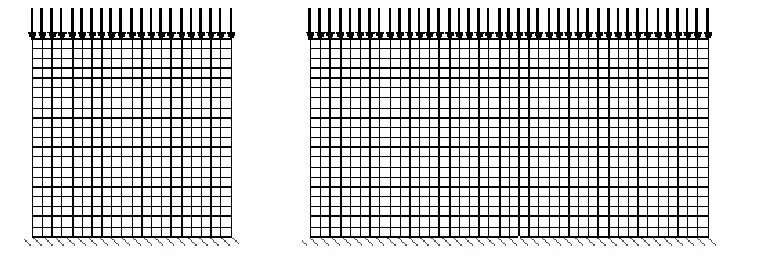
To be able to compare the solutions and to discuss the details concerning constructing the structure using proposed here ways of construction (e.g. making various static scheme) the same examples are taken into consideration as it was in[3], which means the internally ribbed plate is considered (Fig. 1). The problem is discussed for one direction (for the second orthogonal direction the solution is the same). This means we have to consider the two dimension problem. The FE mesh (20 x 20 and 20 x 40) is shown in the Fig. 2.

Fig. 2 FE mesh for considered examples

The material data and dimensions are given as dimensionless results, which means the qualitative analysis is presented here. The cross-section has the mass amounting to 30% of the total volume (a = 0.3). The available mass of the structure may be written as:

m0 = am(TE – AE – SWE ) + AE +SWE (9)

(4)

where TE is the total number of the elements, AE is the number of elements where mass is assumed as equal to one and

SWE is the number of elements where stronger or weaker material is imposed. Some examples which illustrate suitability of proposed method is presented below.

Similar to[3] the updating scheme of the Young’s modulus is a function of the material density of the element j

in every optimization step

å

= ÷÷ø

ö çç è æ

= 3

1 3 0

n h

j j

j E

E ( ) ( )

r r

r (10)

To compare the solutions the threshold functions are defined as

TF1=0.1ai, TF2=0.0125ai (11)

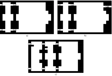
Fig. 3 Initial state a), previous topology b), present topology with “x” c)

In the Fig. 3a the initial state is shown. Initially the material was imposed in the top and bottom covers and additionally it was imposed as a core of four ribs. In this case we do not consider the mass in the elements marked by “x”. This is the example taken from[3] to compare with the present research. The 0/1 topology for the case shown in the Fig. 3a without “x” elements is presented in the Fig. 3b. There is no connections of two ribs with covers and the left rib has no exact vertical shape. When we add the mass into the elements marked by “x” the ribs becomes thinner and the left rib is exact vertical with only two inclusions (two material elements).

1.000 1.000 1.000 1.000 1.000 1.000 1.000 1.000 1.000 1.000 1.000 1.000 1.000 1.000 1.000 1.000 1.000 1.000 1.000 1.000

1.000 0.876 0.999 1.000 0.871 0.903 1.000

1.000 1.000 1.000 0.854 0.934 0.937

0.925 0.898 0.982 0.882 0.884 1.000 0.868 0.860 0.919 0.912

0.895 0.866 0.858 0.931 0.881 0.898 0.969 0.896 0.909 0.918

0.890 0.877 0.936 0.880 0.908 0.981 0.923 0.906 0.946

0.927 0.921 1.000 0.907 0.947 1.000 0.969 0.919 0.999

0.977 0.882 0.961 1.000 0.940 0.985 1.000 1.000 0.961 1.000

1.000 1.000 1.000 1.000

0.970 0.880 0.948 1.000 0.961 0.982 1.000 1.000 0.952 1.000

0.911 0.923 1.000 0.919 0.940 1.000 0.956 0.908 0.995

0.861 0.886 0.921 0.882 0.895 0.936 0.905 0.890 0.941

0.868 0.880 0.865 0.872 0.887 0.872 0.889 0.911

0.860 0.855 0.860 0.854 0.858 0.861 0.854 0.896 0.903

0.876 0.882 0.852 0.854 0.911 0.929

0.990 0.871 0.893 1.000

1.000 1.000 1.000 1.000 1.000 1.000 1.000 1.000 1.000 1.000 1.000 1.000 1.000 1.000 1.000 1.000 1.000 1.000 1.000 1.000

a)

1.000 1.000 1.000 1.000 1.000 1.000 1.000 1.000 1.000 1.000 1.000 1.000 1.000 1.000 1.000 1.000 1.000 1.000 1.000 1.000

1.000 0.919 1.000 1.000 0.914 0.948 1.000

X X X 0.979 0.982

0.972 0.943 1.000 0.927 0.929 1.000 0.912 0.905 0.964 0.957

0.943 0.912 0.904 0.983 0.930 0.946 1.000 0.944 0.954 0.964

0.940 0.922 0.986 0.928 0.955 1.000 0.971 0.951 0.992

0.975 0.964 1.000 0.954 0.993 1.000 1.000 0.964 1.000

1.000 0.927 1.000 1.000 0.986 1.000 1.000 1.000 1.000 1.000

1.000 1.000 1.000 1.000

1.000 0.926 0.993 1.000 1.000 1.000 1.000 1.000 0.997 1.000

0.957 0.968 1.000 0.964 0.986 1.000 1.000 0.953 1.000

0.907 0.932 0.967 0.928 0.941 0.982 0.951 0.935 0.986

0.914 0.926 0.911 0.919 0.934 0.919 0.934 0.957

0.906 0.906 0.908 0.942 0.949

0.922 0.928 0.956 0.974

1.000 0.917 0.938 1.000

1.000 1.000 1.000 1.000 1.000 1.000 1.000 1.000 1.000 1.000 1.000 1.000 1.000 1.000 1.000 1.000 1.000 1.000 1.000 1.000

b)

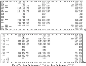
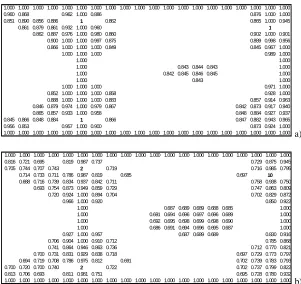
Fig. 4 Topology for imposing “1” a), topology for imposing “2” b)

(5)

How works the procedure we can notice analyzing Fig. 4 where the 11th step for both cases is shown (in the Fig. 3 we had 12th_{step). In the Fig 4a and 4b we have examples taken from the Fig 3a (with “x”). The values of the density in the Fig.}

4a are smaller in comparison to the Fig. 4b where in “x” elements two times stronger material was imposed than it was imposed in the case shown in the Fig. 4a. This means stronger material is a cause of the faster accumulating material and for example the right rib becomes more vertical (in this case we can say the optimization process is faster and gives “better” topology). It is clear imposing the stronger material we improve the topology. To continue our considerations let’s try to impose the additional material in symmetry manner in lower part of the ribs and let’s analyse the topology for the previous to 0/1 distribution step. When we add the same material or two times stronger the same as it was in the Fig. 4 is observed.

1.000 1.000 1.000 1.000 1.000 1.000 1.000 1.000 1.000 1.000 1.000 1.000 1.000 1.000 1.000 1.000 1.000 1.000 1.000 1.000

1.000 0.802 0.942 0.777 0.977 0.801 0.824 0.956

10 10 10 0.779 0.857 0.861

0.853 0.823 0.920 0.810 0.812 0.960 0.795 0.785 0.843 0.836

0.822 0.791 0.784 0.863 0.811 0.828 0.906 0.825 0.833 0.843

0.818 0.801 0.864 0.808 0.837 0.914 0.852 0.831 0.871

0.854 0.842 0.942 0.833 0.875 1.000 0.898 0.845 0.925

0.905 0.808 0.884 1.000 0.868 0.917 1.000 0.946 0.888 0.978

1.000 1.000 1.000 1.000

0.905 0.799 0.864 1.000 0.888 0.913 1.000 0.940 0.877 0.977

0.853 0.835 0.949 0.844 0.872 0.999 0.894 0.832 0.922

0.816 0.801 0.869 0.813 0.833 0.906 0.848 0.815 0.868

0.820 0.786 0.864 0.811 0.822 0.893 0.820 0.815 0.840

0.852 0.797 0.916 0.806 0.807 0.943 0.791 0.779 0.823 0.834

10 10 10 0.779 0.839 0.862

1.000 0.798 0.935 0.779 0.961 0.799 0.821 0.970

1.000 1.000 1.000 1.000 1.000 1.000 1.000 1.000 1.000 1.000 1.000 1.000 1.000 1.000 1.000 1.000 1.000 1.000 1.000 1.000

Fig. 5 Symmetry case topology for imposing “10”

In the Fig. 5 ten times strong material is applied and we can see that very strong material is rounded by weaker material. Why? Because this ten times stronger material is too strong and it is be able to care the large majority of the load. Additionally something like joints we can find in these places when we have imposed such strong material, what can be seen in the Fig. 6 when 0/1 distribution is presented.

Fig. 6 Topology for 0/1 ditribution

The structure becomes mechanism and this is why the strain energy is increasing in this case for imposing the stronger material. From the other hand such constructing the structure may be useful if we choose the place where we impose the stronger material and we will able to control the move (the displacements) of the structure. It is worth to notice the differences between the topology in the step just before 0/1 distribution for the case taken from Fig. 5 when in lower part instead imposing “10” we impose “1” only. Around stronger material (“10”) the density increases if we compare the numbers with the Fig. 5. The same is around the “1” material which is placed in the same elements as earlier “10” was imposed (Fig. 5). This means: when from the structure we remove very strong material (“10”), the structure start to homogenize all the material, especially it is clear around stronger material.

The structure with 3 ribs instead 4 is discussed below (the second rib going from right to left in the Fig. 3a was removed). The symmetry case is considered. In the Fig. 7 there is shown the optimization step just before 0/1 distribution when additionally very strong material was imposed not far away from right top corner. In this figure some material of density over 0.7 wanted to connect with the right rib, trying to create additional rib and connections between two left ribs are observed.

(6)

We should remember that initial distribution of material presented in the Fig. 3a is valid for all the examples as long as proper number of ribs is considered.

1.000 1.000 1.000 1.000 1.000 1.000 1.000 1.000 1.000 1.000 1.000 1.000 1.000 1.000 1.000 1.000 1.000 1.000 1.000 1.000

1.000 0.787 0.824 0.970 0.760 0.810 0.977 1.000

2 0.770 0.756 2 0.795 1.000 0.890

0.909 0.872 0.792 0.961 0.824 0.769 10

0.872 0.834 0.824 0.912 0.840 0.838 1.000 0.849

0.863 0.805 0.750 0.849 0.921 0.854 0.751 0.828 0.969 0.919

0.898 0.806 0.901 1.000 0.882 0.779 0.931 0.992

0.947 0.839 0.948 1.000 0.909 0.952 1.000

1.000 1.000 0.752 0.753 1.000

1.000 1.000 0.752 0.757 0.761 0.758 1.000

1.000 1.000 0.753 0.759 0.763 0.759 1.000

1.000 1.000 0.756 0.759 0.756 1.000

0.945 0.831 0.907 1.000 0.946 0.752 0.933 1.000

0.894 0.794 0.882 1.000 0.899 0.758 0.883 0.989

0.858 0.787 0.844 0.922 0.859 0.757 0.756 0.794 0.867 0.933

0.865 0.808 0.825 0.909 0.838 0.770 0.812 0.869 0.904

0.899 0.835 0.796 0.956 0.818 0.777 0.823 0.878 0.896

2 0.766 0.758 2 0.776 0.820 0.894 0.923

1.000 0.792 0.819 0.968 0.772 0.768 0.809 0.869 1.000

1.000 1.000 1.000 1.000 1.000 1.000 1.000 1.000 1.000 1.000 1.000 1.000 1.000 1.000 1.000 1.000 1.000 1.000 1.000 1.000

Fig. 7 Topology for three ribs

2 2

10

2 2

a) b)

2 2 2

c)

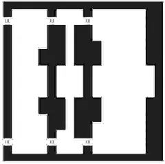
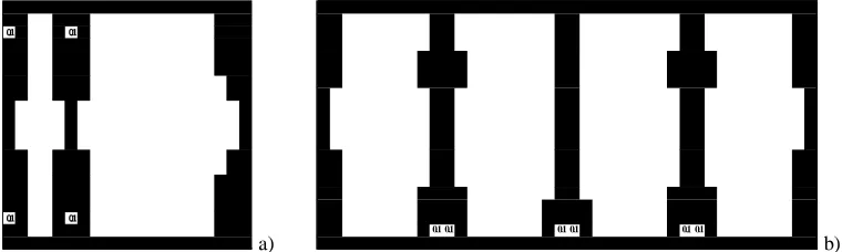
Fig. 8 Topology for three ribs a), topology for three ribs and additionally strong material b), topology for four ribs

Fig. 8a and Fig. 8b show the optimal topologies for three ribs, but in the case of Fig. 8b additionally very strong material was added. This is the black and white mode of the next step to presented in the Fig. 7, where the number mode was used. For making comparison in the Fig. 8c the solution for four ribs is shown. It can be noticed, that removing the rib is a cause of enlarging mainly the right rib and additionally the left rib too. Imposing very strong material in the right corner have changed a little the topology (from some elements in the top part the material was removed). This very strong material we can treat as joint and may be used for controlled destruction of the structure.

Next investigations deals with topology analysing during the decreasing number of ribs. As the first we will discuss the structure with two ribs and finally with one rib. Analysing Fig. 9 we can see how material wants to make the wide ribs to support both covers. Imposing stronger material we let the base material to be weaker in the neighbour of stronger material. Some material is left between two ribs as a core of the next rib, but it is not enough material to create

(7)

the rib. When we observe 0/1 distribution (Fig. 10) it is clear that to fast material was removed from the left-down corner in the left picture, which means the postprocessing sometimes is needed.

1.000 1.000 1.000 1.000 1.000 1.000 1.000 1.000 1.000 1.000 1.000 1.000 1.000 1.000 1.000 1.000 1.000 1.000 1.000 1.000

0.960 0.868 0.962 1.000 0.886 0.876 1.000 1.000

0.851 0.890 0.856 0.886 1 0.862 0.865 1.000 0.945

0.861 0.879 0.861 0.932 1.000 0.960 1

0.862 0.887 0.976 1.000 0.980 0.860 0.902 1.000 0.901 0.900 1.000 1.000 0.997 0.875 0.889 0.998 0.956 0.866 1.000 1.000 1.000 0.849 0.845 0.967 1.000

1.000 1.000 1.000 0.989 1.000

1.000 1.000

1.000 0.843 0.844 0.843 1.000

1.000 0.842 0.845 0.846 0.845 1.000

1.000 0.843 1.000

1.000 1.000 1.000 0.971 1.000

0.852 1.000 1.000 1.000 0.858 0.928 1.000

0.888 1.000 1.000 1.000 0.883 0.857 0.914 0.963 0.846 0.879 0.974 1.000 0.979 0.867 0.842 0.873 0.917 0.940 0.865 0.857 0.933 1.000 0.958 0.848 0.884 0.927 0.937

0.845 0.866 0.848 0.884 1 0.866 0.847 0.882 0.943 0.965

0.956 0.853 0.957 1.000 0.900 0.873 0.924 1.000

1.000 1.000 1.000 1.000 1.000 1.000 1.000 1.000 1.000 1.000 1.000 1.000 1.000 1.000 1.000 1.000 1.000 1.000 1.000 1.000 _a) 1.000 1.000 1.000 1.000 1.000 1.000 1.000 1.000 1.000 1.000 1.000 1.000 1.000 1.000 1.000 1.000 1.000 1.000 1.000 1.000

0.816 0.721 0.695 0.819 0.987 0.737 0.729 0.875 0.945

0.705 0.744 0.707 0.743 2 0.719 0.716 0.985 0.795

0.714 0.733 0.711 0.786 0.987 0.819 0.685 0.697 10

0.688 0.716 0.739 0.834 0.937 0.842 0.711 0.758 0.938 0.750 0.693 0.754 0.873 0.949 0.859 0.729 0.747 0.863 0.809

0.720 0.924 1.000 0.894 0.704 0.702 0.829 0.872

0.966 1.000 0.920 0.850 0.922

1.000 0.687 0.689 0.689 0.688 0.685 1.000

1.000 0.691 0.694 0.696 0.697 0.696 0.689 1.000 1.000 0.692 0.695 0.698 0.699 0.698 0.690 1.000 1.000 0.686 0.691 0.694 0.696 0.695 0.687 1.000 0.927 1.000 0.957 0.687 0.689 0.689 0.830 0.916

0.706 0.904 1.000 0.910 0.712 0.785 0.868

0.741 0.864 0.946 0.863 0.736 0.712 0.770 0.821

0.700 0.731 0.831 0.929 0.838 0.718 0.697 0.729 0.773 0.797 0.694 0.719 0.708 0.786 0.975 0.812 0.691 0.702 0.739 0.783 0.793

0.700 0.720 0.700 0.740 2 0.722 0.702 0.737 0.799 0.822

0.813 0.706 0.693 0.811 0.981 0.751 0.695 0.728 0.780 0.932 1.000 1.000 1.000 1.000 1.000 1.000 1.000 1.000 1.000 1.000 1.000 1.000 1.000 1.000 1.000 1.000 1.000 1.000 1.000 1.000_b)

Fig. 9 Topology for two ribs: with some additional points with “1” a), with “2” and “10”b),

1

2

10

2

Fig. 10 The same as in Fig. 9 example for the next step in black and white notation

As the next example the topologies for one rib is considered. Similar to the previous example, but with only right rib. Of course the strong material “10” is imposed, quite like in the previous examples. The strong material preserve the same shape as in the previous examples, but at a left side the rib is increasing (Fig. 9). For making the topology smoother TF2 was used for the case from Fig. 11b. The black and white topologies were obtained within 11th steps and

within 84th steps for the solutions in the Fig. 12 a and in the Fig. 12b respectively. It is clear TF1 is not able to produce

smooth topology and this is why TF2 is needed and the topology obtained using it is “more optimal” because the strain

energy is less than for the case when TF1 is used.

In presented in the Fig. 13 examples instead stronger the weaker material (ten times weaker) was imposed in marked places. The Fig. 13a is similar to the Fig. 8a. We can observe how changes topology. Instead making the joints the procedure let to surround the weaker material by the base material. Finally, the example for the mesh shown in the Fig. 2 on the right side is presented for imposing the weak material. It was a situation where before imposing weaker material there was no material in these regions and there was no connections among three ribs and lower cover.

(8)

1.0 1.0 1.0 1.0 1.0 1.0 1.0 1.0 1.0 1.0 1.0 1.0 1.0 1.0 1.0 1.0 1.0 1.0 1.0 1.0

0.8 0.7 0.6 0.6 0.8 0.8

0.7 0.7 0.7 0.6 0.9 0.7

0.7 0.7 0.7 0.7 0.6 10

0.7 0.7 0.7 0.6 0.6 0.7 0.8 0.7

0.7 0.7 0.7 0.7 0.6 0.6 0.7 0.8 0.7

0.7 0.7 0.7 0.7 0.7 0.6 0.6 0.6 0.7 0.8

0.6 0.7 0.7 0.7 0.7 0.7 0.6 0.6 0.6 0.7 0.8

0.6 0.7 0.7 0.7 0.7 0.7 0.6 0.6 0.6 0.6 1.0

0.6 0.7 0.7 0.7 0.7 0.7 0.7 0.6 0.6 0.6 0.6 1.0

0.6 0.7 0.7 0.7 0.7 0.7 0.7 0.6 0.6 0.6 1.0

0.6 0.7 0.7 0.7 0.7 0.7 0.6 0.6 0.6 0.7 0.8

0.6 0.7 0.7 0.7 0.7 0.6 0.6 0.6 0.7 0.8

0.6 0.7 0.7 0.7 0.7 0.6 0.6 0.7 0.7

0.7 0.7 0.7 0.7 0.6 0.6 0.6 0.7 0.7

0.6 0.7 0.7 0.7 0.6 0.6 0.7 0.7 0.7

0.7 0.7 0.7 0.6 0.6 0.7 0.7 0.7

0.8 0.7 0.6 0.6 0.7 0.8

1.0 1.0 1.0 1.0 1.0 1.0 1.0 1.0 1.0 1.0 1.0 1.0 1.0 1.0 1.0 1.0 1.0 1.0 1.0 1.0

1.0 0.9 0.9 0.9 1.0 1.0

0.9 0.9 0.9 1.0 0.9

0.9 0.9 0.9 0.9 10

0.9 0.9 0.9 0.9 0.9 1.0 0.9

0.9 0.9 0.9 0.9 0.9 0.9 1.0 0.9

0.9 0.9 0.9 0.9 0.9 0.9 0.9 1.0

0.9 0.9 0.9 0.9 0.9 0.9 1.0 1.0

0.9 0.9 0.9 0.9 0.9 0.9 1.0

0.9 0.9 0.9 0.9 0.9 0.9 0.9 1.0

0.9 0.9 0.9 0.9 0.9 0.9 1.0

0.9 0.9 0.9 0.9 0.9 0.9 0.9 1.0

0.9 0.9 0.9 0.9 0.9 0.9 1.0

0.9 0.9 0.9 0.9 0.9 0.9 0.9

0.9 0.9 0.9 0.9 0.9 0.9

1.0 0.9 0.9 0.9 0.9 1.0

1.0 1.0 1.0 1.0 1.0 1.0 1.0 1.0 1.0 1.0 1.0 1.0 1.0 1.0 1.0 1.0 1.0 1.0 1.0 1.0

a) b)

Fig. 11 Topology for one rib only for TF1 a) and for TF2 b)

10

Fig. 12 Black and white topology for one rib only for TF1 a) and for TF2 b)

0.1 0.1

a)

0.1 0.1 0.1 0.1 0.1 0.1 b)

Fig. 13 Black and white topology for imposing weaker material

CONCLUSION

Proposed procedure may be useful for the smart design process. Imposing stronger material the designer is able to have a structure with some kind of joints, which can help to control the destruction process and to change when it is needed the static scheme of the structure. Imposing weaker material in those places where there is a shortage of material (where during the optimization process there was no possible to give the material) the designer is able to fulfils the empty places automatically, because weaker material is rounded by normal material. Proposed procedure (which can be called the smart procedure) give us finally the optimal topology of the structure, even during the destruction process.

REFERENCES

1. Kutyłowski, R., “On nonunique solutions in topology optimization”, Structural and Multidisciplinary Optimization, Vol. 23, 2002, pp. 398-403

2. Bendsøe, M. P., Sigmund, O., Topology optimization, Theory, methods and applications, Springer Verlag, Berlin, Heidelberg, New York, 2003.

3. Kutyłowski, R., “Topology of Internal Ribbed Plates Cross Section”. Proc. of the SMiRT 15 Conference, pp. IV-153 – IV-160, Seoul, Korea, August 1999.