Changhai Ou
1, Xinping Zhou
2and Siew-Kei Lam
11 School of Computer Science and Engineering,
Nanyang Technological University, Singapore,[email protected],[email protected] 2 Beijing Unionpay Card Technology Co., Ltd, China,[email protected]
Abstract. Side-channel attacks and evaluations typically utilize leakage models to extract sensitive information from measurements of cryptographic implementations. Efforts to establish a true leakage model is still an active area of research since Kocher proposed Differential Power Analysis (DPA) in 1999. Leakage certification plays an important role in this aspect to address the following question: "how good is my leakage model?". However, existing leakage certification methods still need to tolerate assumption error and estimation error of unknown leakage models. There are many probability density distributions satisfying given moment constraints. As such, finding the most unbiased and most reasonable model still remains an unre-solved problem. In this paper, we address a more fundamental question: "what’s the true leakage model of a chip?". In particular, we propose Maximum Entropy Distribution (MED) to estimate the leakage model as MED is the most unbiased, objective and theoretically the most reasonable probability density distribution con-ditioned upon the available information. MED can theoretically use information on arbitrary higher-order moments to infinitely approximate the true leakage model. It well compensates the theory vacancy of model profiling and evaluation. Experimen-tal results demonstrate the superiority of our proposed method for approximating the leakage model using MED estimation.
Keywords: information theory·maximum entropy·maximum entropy distribution
·leakage model·leakage certification·side channel attack
1
Introduction
Side-channel attacks, which aim to extract secret information that are unintentionally leaked in a cryptographic implementation, have been regarded as one of the most
impor-tant threats against the security of embedded devices [RSV+11]. Power attacks, the most
classic one of this family, can be divided into two categories: profiled attacks and
non-profiled attacks. Non-non-profiled attacks such as Differential Power Analysis (DPA) [KJJ99],
classify measurements (i.e. power traces) according to the intermediate values, and then calculate the differences. The correct key corresponds to the most obvious differential value (i.e. peak). The advantage of non-profiled attacks is that the attacker does not require prior knowledge of the leakage model.
Standard profiled attacks include Template Attacks (TA) [CRR02,RO04] and
stochas-tic models [SLP05] as stated in [SKS09]. They include two stages: leakage profiling and
exploiting. The attacker needs to profile a leakage model before exploiting the leakage to recover the key. The true leakage of the cryptographic hardware is unknown and difficult to derive, and normal distribution is often used as the hypothetical model. Actually, the true leakage model may not well follow it. Hypothetical models such as Hamming weight [BCO04], Hamming distance [PSDQ05] and Switch [Pee13], can also be used to
improve the efficiency. Exploring a true leakage model continues to be an active area of research.
In this paper, we aim to investigate the most unbiased, most reasonable and realistic
leakage model, in order to address the question: "what’s the true leakage model of a
chip?". Existing works in side-channel attacks and evaluations (e.g. leakage detections
and assessments) have also attempted to propose such a model, but without thorough study and suitable answers. In the following section, we will discuss these existing works along with leakage certification methods, before describing the main contributions of our work.
1.1
Related Works
Side channel attacks. A good leakage model has a significant impact on the effectiveness
of side channel attacks. Many recent works have been undertaken to accurately profile the leakage model. However, most of them only considered first- and second-order moments (i.e. mean and variance) when profiling probability density distribution. This typically
happens in Template Attack [RO04], which takes advantage of an off-line learning phase
in order to estimate the leakage model. Since the true leakage model is unknown, the profiling methods are typically based on some assumptions on the leakage distribution
(e.g. Gaussian noise) as in [DSV14], which is not representative of the true leakage.
Flament et. al. discussed probability density function estimation for side-channel attacks
in [FSJL+10]. They compared parametric estimation and histogram estimation, but did
not consider information on higher-order moments.
Side channel evaluations. For attackers, the accuracy of the leakage model affects
the effectiveness of the attack. For evaluators, the accuracy of leakage model affects the
re-liability of the evaluations (e.g. Success Rate (SR) and Guessing Entropy (GE) [SMY09]).
Since model errors provide evaluators with a false security level. Leakage detections, which relate to the concrete security level of an implementation given a model, are very important tools for side-channel evaluation. Unlike the above-mentioned side-channel at-tacks that are based on an assumption model, leakage detection tests such as Welch’s
t-test [DCE16,Rep16,BPG18], Normalized Inter-Class Variance (NICV) [BDGN14],
cor-relationρ-test [DS16] andχ2test [MRSS18], use a bounded moment model [JS17]. They
try to quantify the security of an implementation, of which the model reflects the leakage of target device. Leakage detection and assessment have been performed before
cryp-tographic algorithms are implemented on devices in [Rep16] and [CGD18]. These tests
aim to detect the presence of leakage, without regards to whether the leakage can be exploited. Leakage assessments seek a standard approach that enables a fast, reliable and
robust evaluation of the side-channel vulnerability of the given devices [SM15]. They can
be regarded as an extension of leakage detection, which also require a bounded moment model rather than a true leakage distribution model. The above-mentioned works usually
consider moments that are less than 4th order. Higher-order moments (larger than 4)
leakage detection and assessments (e.g. [JS17, MW15, RGV17] and [SM15]) are seldom
studied.
Leakage certifications. The effectiveness of both side-channel attacks and
evalua-tions rely heavily on the true leakage model. However, this model is usually unknown. The following question underpins all the efforts that range from assuming a good leakage model (e.g. Hamming weight model and Hamming distance model) to profiling a good leakage model (e.g. normal distribution model and higher-order moments model used
in higher-order attacks [Mor12, MS16]): How good is the leakage model? The answer
to this question can be traced back to the complete evaluation framework proposed by
Standaert et al. in [SMY09]. The authors used Mutual Information (MI) to quantify the
Information (PI) to estimate the MI biased by side-channel adversary’s model [RSV+11]. In this case, the accuracy of the model determines the closeness of PI and MI. To
bet-ter answer the question above, Durvaux et al. in [DSV14] proposed leakage certification,
which attempted to solve the fundamental problem that all evaluations were potentially biased by both assumption and estimation errors. They also tried to quantify the leakage of a chip and certify that the amount of information extracted was close to the maximum value that would be obtained with a perfect model. This work was further improved in [DSP16].
1.2
Our Contributions
Existing works on side-channel attacks and evaluations have incessantly pursued a true leakage model. While existing leakage certification methods can provide a reasonable leakage model, they do not alleviate the attacker or evaluator from having to deal with model assumption error and estimation error. Moreover, the probability density distribu-tion model under higher-order moments has not been discussed in existing works. Finally, even though there are numerous probability density distributions satisfying given moment constraints, achieving the most unbiased, most reasonable and least hypothetical leakage model still remains an unresolved problem.
To address the shortcomings of existing work on leakage certification, we propose Maximum Entropy Distribution (MED) to estimate the true leakage model of a chip. MED is the most unbiased, random, uniform and theoretically the most reasonable probability density distribution conditioned upon the available information. Here MED presents the probability density function assigned by using principle of maximum entropy. MED can theoretically use information on arbitrary higher-order moments to infinitely approximate the true distribution of leakage, rather than assume a leakage model. To the best of our knowledge, this is the first work that considers information on higher-order moments when estimating probability density distribution. Experimental results demonstrate the superiority of our proposed method for approximating the leakage model using maximum entropy distribution estimation.
1.3
Organization
The rest of the paper is organized as follows. Information entropy, maximum entropy and leakage certification are introduced in Section 2. In Section 3, MED, including its esti-mation, parameter determination and fitting performance between estimated Probability Density Function (PDF) model and true leakage, is given. Then, we use Newton-Raphson nonlinear programming optimization method to fit MED with true distribution in Section 4. The specific algorithm and the optimal choice of histogram bins are also given in this section. Experiments are performed on simulated traces and measurements of
AT-Mega644P micro-controller provided in [DSP16] in Sections 5 and 6 to demonstrate the
efficiency of our MED. Finally, we conclude the paper in Section 7.
2
Preliminaries
2.1
Information Entropy
Information entropy is a very important concept in information theory. Let X be a
discrete random variable consisting of n observations of x = (x1, x2, . . . , xn), and the
(or uncertainty) as
H(x) =−
n X
i=1
pilnpi (1)
in [Sha48], which was also denoted as self-information. Here 0≤pi ≤1, and ln denotes
the logarithmic function. IfXis a continuous random variable, then the Shannon entropy
is
H(x) =−
Z b
a
f(x)lnf(x)dx. (2)
Here [a, b] is the integral interval, andf(x) is the probability density function. Information
entropy is widely used in side-channel analysis such as Mutual Information Analysis (MIA) [GBTP08]. Self information of measurements can be used to quantify the leakage model of a chip.
2.2
Maximum Entropy Principle
Information theory provides a constructive criterion for setting up probability distribu-tions on the basis of partial knowledge and leads to a type of statistical inference which
is called the maximum entropy estimate [Jay57]. Maximum entropy estimation is the
most unbiased or most uniform probability distribution conditioned upon the available
information [SGUK08]. Maximum entropy here means maximizing information entropy
in Eq. 1or Eq. 2.
There is an implicit constraint in Eq. 1 where
n X
i=1
pi= 1. (3)
The direct problem is to determinepconditioned upon Eq. 3. As detailed by
Munirath-nam et al. in [SKR00], maximum entropy solved this problem by the maximization of
Shannon entropy (uncertainty measure) of probabilities given in Eq. 1. By considering
La-grange multipliers, in order to maximize the entropy, the probabilitiesp= (p1, p2, . . . , pn)
should satisfy
ϕ(p1, p2, . . . , pn) =−
n X
i=1
pilnpi+λ
n X
i=1
pi−1
!
. (4)
The purpose of this paper is to profile the true leakage model from the observed samples. So, we use observer to represent side-channel attackers and evaluators. By differentiating
ϕwith respect topi, the observer gets
∂ϕ
∂pi
=−(lnpi+ 1) +λ= 0. (5)
That is, (lnpi+ 1) =λ, we deduce thatpi=eλ−1. When combined with Eq. 3, we obtain
Pn
i=1eλ−1= 1. So,
λ=ln
1
n
+ 1. (6)
Finally, we obtainpi=n1. That is to say, if we don’t make any further assumptions onpi,
2.3
Leakage Certification
Side-channel attacks and evaluations require a perfect model to extract all information from the leakage measurements. However, the leakage model is never perfect with errors arising from assumption and estimation. Durvaux et al. proposed the pioneering leakage
certification in [DSV14] and improved it in [DSP16]. Leakage certification aims to bound
and reduce the assumption and estimation errors, thus providing a good enough leakage model for attacks and evaluations.
Assumption error. Since the true leakage model of devices is unknown, the observer
has to establish an assumption leakage model before he performs attacks or evaluations. For example, Gaussian model including mean and variance are used in Template Attack
[RO04], and Hamming weight model in CPA [BCO04]. These models include subjective
assumptions and can easily lead to assumption error. A good model should reflect the basic information of the leakage, but it is not the real leakage model of the chip. The goodness of fit of these two models can be quantified by hypothesis testing.
Estimation error. The estimation error is the difference between the estimated
pa-rameters and true papa-rameters of the leakage model. The main cause of this error is that the number of measurements is insufficient, which makes the probability density distribu-tion estimadistribu-tion deviate from the true distribudistribu-tion. Typical estimadistribu-tion error is shown in Fig. 1, where two models estimated from samples deviate from the true distribution. It can be observed that Model 1 deviates further from the true leakage model than Model 2. Estimation error can be made arbitrarily small through more measurements and using
cross validation techniques [DSP16].
-40 -30 -20 -10 0 10 20 30 40 power consumption
0 0.02 0.04 0.06 0.08 0.1 0.12
probability density
sample distribution biased Model 1 biased Model 2
Figure 1: Estimation errors in leakage model profiling.
Cross-validation. For each plaintext z, the observer randomly acquires samples
and estimates the dth order mean ˆµd using cross validation. Suppose that k-fold cross
validation is used andnmeasurements are acquired. Measurements are divided intok
non-overlapping folds of approximately the same size as introduced in [DSP16]. The observer
then selects thejth(1≤j≤k) fold as the validation set and otherk−1 folds as profiling
set. The observer then randomly generates samples from the estimated leakage model.
Each repetition generates adthorder moment estimate ˜md,(j)
z . Thedthorder mean ˜µd of
real samples is processed in the same way. Thus,
ˆ
µd
z= ˆEj
ˆ md,(j)
z
,σˆd z=
r
ˆ
varj
ˆ md,z(j)
,
˜ µdz= ˜Ej
˜ md,z(j)
,σ˜dz= r
˜
varj
˜ md,z(j)
.
(7)
is performed as:
∆d
z=
ˆ
µd
z−µ˜dz q
(ˆσd z)
2
+(˜σd z)
2 k
. (8)
Let CDFt denote the Cumulative Distribution Function (CDF) in t-test, df denote the
number of freedom degrees (see Section 4.1 in [DSP16]). The probability of observed
difference coming from the effects of estimation is:
p= 2× 1−CDFt
∆dz, df
. (9)
The probabilityponly indicates that the difference between true samples and simulated
samples has statistical significance. It doesn’t reflect how large the difference is. The
largerpis, the smaller the probability of estimation error. Leakage certification test uses
information on higher-order moments to profile bounded moment leakage model [JS17],
rather than making assumptions on the leakage distribution.
3
Maximum Entropy Distribution Estimation
A perfect leakage model can accurately reflect the leakage of devices and improve the effectiveness of side-channel attacks and security evaluations. However, such perfect mod-els are generally unknown. Density estimation techniques, such as Maximum Entropy
Distribution (MED) [XM10], have to be used to approximate the leakage distribution.
3.1
Maximum Entropy Distribution
Suppose that geometrical moments are used, the maximum entropy of the random variable
Xcan be obtained by maximizing Shannon’s entropy (see Eq. 1) subject to the constraints:
Z
xif(x)dx=µi, i= 0, . . . , N (10)
whereµi is the expectation value calculated from samples (e.g. µ0= 1). N denotes that
the firstN + 1 moment constraints (µ0, µ1, . . . , µN) are used in our side-channel attacks
or evaluations. This can be expressed as the Lagrangian:
L=−
Z
f(x)lnf(x)dx+ (λ0+ 1)
Z
f(x)dx−1
+
m X
i=1 λi
Z
xif(x)dx−µi
.
(11)
Here, λ = (λ0, λ1, . . . , λm) are unknown Lagrange multipliers, and ln denotes natural
logarithm. The setting of coefficient (λ0+ 1) is to facilitate the solution ofλ. Maximum
entropy usually occurs at the extreme point of function λ. By differentiating L with
respect to f(x), we have
∂L
∂f(x) =−
Z
[lnf(x) + 1]dx+ (λ0+ 1)
Z
dx+
m X
i=1 λi
Z
xidx. (12)
We set ∂L
∂f(x)= 0 and obtain
−[lnf(x) + 1] + (λ0+ 1) +
m X
i=1
By transposition, we further get
lnf(x) =λ0+
m X
i=1
λixi. (14)
Finally, we derive the maximum entropy probability density function (MED) as
f(x) =exp λ0+
m X
i=1 λixi
!
. (15)
Maximum entropy accommodates information on higher-order moments and therefore facilitates a higher quality probability density function model. The observer does not make any assumptions on the leakage model except the moment information from the
samples, which also shows the objectivity and rationality off(x).
3.2
Parameter Determination
We have derived the maximum entropy probability density function in Section3.1. We
can get the corresponding expression after solving the Lagrange Multipliers inf(x). Since
Z
f(x)dx=
Z
exp λ0+
m X
i=1 λixi
!
dx= 1, (16)
by multiplying both sides of the equality bye−λ0, we obtain
e−λ0 =
Z
exp
m X
i=1 λixi
!
dx. (17)
The first unknown Lagrange multiplier can be expressed as:
λ0=−ln
Z
exp
m X
i=1 λixi
!
dx. (18)
By differentiatingλ0with respect to λi (see Eq. 17), we can also get
∂λ0
∂λi
=
Z
xiexp
m X
i=1 λixi
!
dx. (19)
This means, ∂λ0
∂λi =µi. Since
R
exp Pmi=1λixidx= 1, the Lagrange multipliers can be
defined by the sum of residuals:
ri= 1−
R
xiexp Pm
i=1λixi
dx
µiRexp(Pmi=1λixi)dx
(20)
fori= 1,2, . . . , m. The minimum residual can be expressed as:
min R=
m X
i=1
ri. (21)
Suppose that ǫ is the permissible error of the observer. If R < ǫ, then R converges, he
accepts the corresponding Lagrange multipliers λ = (λ0, λ1, . . . , λm) and recovers the
probability density function f(x). The problem of Shannon entropy maximization is a
3.3
Fitting Performance Metrics
Maximum entropy is a monotonic decreasing function, which means that the observer obtains smaller maximum entropy when the algorithm iterates. The probability density
function MED is obtained after R < ǫ. This will be followed by testing whether the
profiled model can accurately reflect the true leakage of device (i.e. test of goodness of fit).
According to the report "Guide to Expression of Uncertainty in Measurement (GUM)"
(see [IO95]), standard uncertainty of the result of measurement corresponding to maximum
entropy is expressed as a standard deviation. By performing maximum entropy estimation on the observations, the expectation and deviation are
ˆ
µ=
Z
xfˆ(x)dx (22)
and
ˆ
σ=
Z
[x−xˆ(x)]2fˆ(x)dx. (23)
Iff(x) approximates the true distribution, ˆµ→µ1and ˆσ→µ2.
Actually, to test whether this model is consistent with the real leakage model, the
leakage certification test of Durvaux et al. (see [DSP16] and [DSV14]) can be employed.
This work performed hypothesis tests on samples generated from the estimated leakage model and real samples to determine if the model can be accepted based on the test
results. Other tests such as Chi-squareχ2[MRSS18] and Root Mean Square Error (RMSE)
[SUK06], can also be used to test maximum entropy probability density distribution. In principle, the more moments are used, the more accurate the model is, and the smaller the error.
In our paper, we combine GUM’s test and Welch’s t-test introduced by Durvaux et al. in [DSV14] to detect estimation error. Specifically, referring to the leakage certification
test of Durvaux et al., we divide the collected measurements intok-folds of approximately
the same size. Each iteration selects a new validation fold and uses otherk−1 folds as
training set. We first find the interval of training set and calculate ˆµand ˆσin GUM’s test.
We then randomly generate samples of the same size as the validation set from this model.
Referring to Eq. 8 and Eq. 9, we carry out Welch’s t-test to quantify the probability of
the difference caused by the estimation error.
4
Nonlinear Programming Optimization
The minimum residual given by Eq. 21 can be solved using nonlinear programming
optimization, which minimizes residual by calculating the least squares of error. If ri is
a linear function for all i, R can be solved by linear least square method. R here is a
non-linear function that can be solved using nonlinear least square method. This is based on the basic principle of using a series of linear least squares to solve nonlinear least square problems.
4.1
Newton-Raphson Method
By combining Eq. 10and Eq. 15, theithorder moment can be expressed as:
Gi(λ) =
Z
xiexp λ0+
m X
i=1 λixi
!
dx=µi (24)
if Eq. 10 is regarded as a function ofλ= (λ0, λ1, . . . , λm). According to [ZH88,MD92],
and higher-order moments
µ′i =Gi(λ)
∼
=Gi λ0+ λ−λ0
T
[gradGi(λ)]λ=λ0
(25)
and solving them iteratively. Here the symbol ’T’ indicates vector or matrix transposition
and symbol ’grad’ indicates gradient function. If the first five moments are taken into
consideration, thenm= 4. Mean, variance, skewness and kurtosis [MS16] are often used
in side-channel attacks. However, very a few papers discussed very higher-order moments
(e.g. [JS17]). Obviously, for nonlinear functions likeR, the observer can solve them using
higher-order Taylor expansions, of whichµ′i is closer toµi.
The work in [MD92] defined two vectors
δ=λ−λ0 (26)
and
v=hµ′0−G0 λ0
, . . . , µ′N−GN λ0
i
T
. (27)
Here the superscript 0 ofλ0represents the number of iterations. The authors then defined
a matrixG by
G=
gnk
=
∂Gn(λ)
∂λk
(λ−λ0)
. (28)
Gis a Hankel matrix, of which
gnk=
Z
xnxkexp
m X
i=1 λixi
!
dx
=
Z
xn+kexp
m X
i=1 λixi
!
dx
=gn+k.
(29)
This meansgnk=gkn. This also means that in order to calculate the first five moments
(m= 4) off(x), we have to calculate G0, . . . ,G8. Solving Eq. 21is equivalent to solving
the linear system of equations:
Gδ=v. (30)
The above is the first iteration ofλ0. The observer obtains the errorδ0ofλ0in probability
density function f(x). Then λ0 is replaced by λ1 = λ0+δ0 and the next iteration is
executed. The iteration continues until δ becomes appropriately small (i.e. R < ǫ). In
principle, the smaller theǫ, the betterf(x) fits the true leakage distribution.
4.2
Algorithm Implementation
We have described the principle of nonlinear programming optimized MED estimation in the previous sub-section. Here we provide the detailed algorithm in Algorithm 1. In our
algorithm, the samples and accuracy serve as inputs, λand maximum entropyM axEnt
are the outputs. There are no other parameters to set, which indicates that our algo-rithm is very simple and does not need to handle the complex parameter optimization
problem. The algorithm first estimates the optimal number of bins hn using function
BinsEstimation(as detailed in Section 4.3). Then, it estimates the probability density
Algorithm 1:Nonlinear programming optimized MED estimate.
Input: samplesxandǫ
Output: estimated parametersλandM axEnt
1 the number of binshn=BinsEstimation(x) ;
2 estimate PDF (p,x) =Histogram(x, hn) ;
3 calculate momentsG1, . . . , GN usingpandx ;
4 λ0=max(x)−min(x) ;
5 while1 do
6 calculatev ;
7 solveGδ=v ;
8 updateλ=λ+δ;
9 updatef(x) andR;
10 if R < ǫthen
11 M axEnt=−Phn
j=1f(xj)lnf(xj);
12 break;
13 end
14 updateG1, . . . , GN usingf(x) andx;
15 end
The outputs of function Histogram include the probability density distribution p and
the mid-points of all binsx.
The purpose of Algorithm 1 is to fit p and f(x) and find the parameters in λ that
satisfies the fitness condition. It is worth noting that our algorithm does not need to set
λ. We only initialize λ0 =max(x)−min(x) as suggested in [MD92]. All λ-s will be
adjusted in the following repetitions. Our algorithm initializes momentsG1, . . . , GN using
pandx. It then calculatesv, solvesGδ=v and updatesλ=λ+δ. It then updatesf(x)
using λ. λand Rwill gradually stabilize after a number of iterations. In this case,f(x)
approximates the distributionp, and the measurement uncertainty in Eq. 22and Eq. 23
approaches the mean and variance of true samples.
For Newton-Raphson method, one of the conditions for iterative convergence is that
G is a non-singular matrix. IfG is singular, then nonlinear programming optimizations
such as damped least square (i.e. Levenberg-Marquardt) method, can also be taken into consideration. Unlike Newton-Raphson method, Levenberg-Marquardt method needs to set several parameters. To optimize these parameters, we need to consider the specific samples and model, which is not easy. Moreover, the algorithm may return a local optimal solution during iteration. In order to find the global optimal solution, Algorithm 1 can be
combined with Simulated Annealing (SA) [GG84] or Genetic Algorithm (GA) [XM10].
4.3
Optimal Bin Width in Histogram
Probability density estimation is a widely-used method for estimating the distribution model of samples. It can be broadly classified to parametric estimation and non-parametric estimation. Parametric estimation is utilized If we have already known what kind of prob-ability density distribution the observed samples follow and only need to determine its parameters. The most commonly used parametric estimation methods are Maximum Likelihood Estimation (MLE) and Bayesian estimation. If we do not know the true distri-bution of the observed samples, we can only use the non-parametric estimation method to estimate its probability density distribution model. The non-parametric estimation
meth-ods mainly include histogram estimation and Kernel Density Estimation (KDE) [Ven10].
density distribution in this paper.
Letκ denote the number of bins in histogram, and x denote the mid-points of bins.
The mid-pointxj of each interval (1≤j≤κ) is often selected as representative value of
this bin [SKR00]. To derive the probability density distribution, the observer needs to
calculate the frequency of each bin. Suppose that he obtains the frequency distribution
ofxas (f1, f2, . . . , fκ) (see [SKR00]). In this case, the expectation value of theith order
moment of samples can be expressed as:
µi=E xi
∼
= 1
κ
κ X
j=1
fjxij. (31)
In order to avoid overflow, the domain of x can also be transformed into interval [0,1]
using equationx′ = (x−xmin)/(xmax−xmin). Herexminandxmaxdenote the minimum
and maximum values of x.
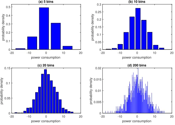
It is difficult to determine the optimal bin width when constructing a histogram. To
illustrate this, we simulate the normal distributionN 0,52
and randomly generate 1000 measurements from this model. The probability density distributions when the number of bins is set to 5, 10, 20 and 200 are shown in Fig. 2. As can be observed, it will be unreasonable to set the number of bins to 5 and 200, as this will lead to the number of bins being either too small or too large. As a result, profiling will lose a lot of information of the distribution. On the other hand, determining whether 10 bins or 20 bins are reasonable
is not straightforward. The authors in [Wan97] suggested that the bin width should be
chosen so that the histogram displays the essential structure of the data, without giving too much credence to the data set at hand.
(a) 5 bins
-20 -10 0 10 20
power consumption
0 0.1 0.2 0.3 0.4 0.5
probability density
(b) 10 bins
-20 -10 0 10 20
power consumption
0 0.05 0.1 0.15 0.2 0.25 0.3
probability density
(c) 20 bins
-20 -10 0 10 20
power consumption
0 0.05 0.1 0.15
probability density
(d) 200 bins
-20 -10 0 10 20
power consumption
0 0.005 0.01 0.015 0.02
probability density
Figure 2: Probability density distribution under different numbers of bins.
considered.
The authors in [Sco79] indicated that the formula for determining the optimal
his-togram bin width should asymptotically minimize the integrated mean squared error. They proposed the following to determine the bin width:
hn=
3.49s
3
√n , (32)
where s was an estimate of the standard deviation and n was the sample size. In
side-channel attacks, we often assume that the leakage follows Gaussian distribution. However, this assumption may be incorrect, or at least inaccurate, since the true leakage model is
unknown. Although Eq. 32 is established on the basis of Gaussian density, fortunately,
it can be also used for non-Gaussian data. Thanks to Scott’s solution, the problem of estimating the bin width in our side-channel attacks can be resolved.
5
Simulated Experiments
5.1
Leakage Function
Our first experiment is performed on simulated measurements. Let HW(·) denote the
Hamming weight function, SBOX(·) denote the SubBytes operation of AES-128, zi
de-note theithplaintext byte andk∗ denote the encryption key byte. The leakage function
is defined as:
li=HW(SBOX(zi⊕k∗)) +θ, (33)
where⊕denotes the XOR operation,li denotes the corresponding leakage sample andθ
denotes the noise component [MOP07] that follows normal distributionN 0,102
.
5.2
Information on Higher-order Moments
Maximum entropy decreases with increase in moment constraints. Since each moment contains information, the uncertainty of the model is reduced if a new moment is added. However, this conclusion is not always established when measurements are limited (as
shown in Table.1). Here 800 measurements are used,ǫis set to 10−8 andC
i denotes the
ithorder moment. The maximum entropy under the constraint of natural moment (C0) is
about 14.6171 and changes to 14.6460 after adding the first-order moment constraint. This means that the maximum uncertainty of distribution varies by 0.0289 after adding the first-order moment. The second-order moment makes the maximum uncertainty decrease
the most followed by the first-order moment. M axEntchanges very little after reaching
9.8123. In this case, the fitting performance also gradually approaches the optimum.
Table 1: Maximum entropy under different constraint sets.
Constraint sets M axEnt
{N} 14.6171
{N,C1} 14.6460
{N,C1,C2} 9.4689
{N,C1,C2,C3} 9.8123
{N,C1,C2,C3,C4} 9.8123
{N,C1,C2,C3,C4,C5} 9.8123
Since we only initializeλ0in our MED, the fitting performance off(x) and true leakage
distribution is not good at the initial iterations. As the number of iterations increases,
the variables inλare constantly updated,f(x) also converges to the true distribution (as
shown in Fig. 3(1)). Finally, the required accuracy is achieved after 10 iterations. The information entropy on different moments is different, as with the fitting
-25 -20 -15 -10 -5 0 5 10 15 20 25
power consumption
0 5 10 15 20 25
probability density
(a) MED under different iterations
iter=1 iter=2 iter=3 iter=4 iter=5 iter=6 iter=7 iter=8 iter=9 iter=10
(b) Fitting performance under different moments
-25 -20 -15 -10 -5 0 5 10 15 20 25
power consumption
0 0.05 0.1 0.15 0.2
probability density
sample distribution leakage function MaxEnt2 MaxEnt3 MaxEnt4 MaxEnt5
Figure 3: MED under different iterations and fitting performance under different mo-ments.
the moments with orders higher than 3. Let MaxEnt2 denotes a set of moments including
{N,C1,C2}, and MaxEnt3 denotes a set of moments including {N,C1,C2,C3}. Similar
notations apply for MaxEnt4 and MaxEnt5. It can be observed from the experimental results in Fig. 3(2) that the higher the orders use, the better the fitting performance
of f(x) and the true distribution. When considering MaxEnt2 and MaxEnt3, f(x) still
deviates from the true distribution of the leakage, and the two have a good fit in MaxEnt4.
The fitting performance in MaxEnt5 is better andf(x) almost passes through the middle
of all bins. On one hand, this indicates that to fit the real leakage distribution, we need to combine the information on all six moments in MaxEnt5. On the other hand, this indi-cates that the information on higher-order moments are limited. It is obvious that there
is still a deviation between the estimated modelf(x) and the true leakage model. This is
mainly due to the small number of samples we use and the large deviation between the sample distribution and real leakage distribution in our experiment. In order to better fit
the real leakage distribution, we can further reduceǫ or consider higher-order moments,
or even use more measurements.
5.3
Fitting Performance
The evaluator can encrypt any number of plaintexts and collect their leakage to profile sufficiently accurate PDF model. Compared to evaluator, the number of measurements obtained by the attacker is limited, so it is important to make full use of the information on them. The number of measurements is also the most important factor in our MED estimation. So, estimating the most reasonable, most unbiased leakage model from the limited model is a very important issue that they needs to be taken into consideration. Here we also compare fitting performance of our MED estimation under different numbers of measurements. The experimental results corresponding to Hamming weight 0 are shown
in Fig. 4, Fig. 5 and Table2.
(a) MED4
-30 -25 -20 -15 -10 -5 0 5 10 15 20 power consmuption 0 0.05 0.1 0.15 0.2 0.25 0.3 probability density iter=9 iter=10 iter=11 iter=12 iter=13 iter=14 (b) MED5
-30 -25 -20 -15 -10 -5 0 5 10 15 20 power consmuption 0 0.05 0.1 0.15 0.2 0.25 0.3 0.35 0.4 probability density iter=9 iter=10 iter=11 iter=11 iter=12 iter=13 iter=14 (c) MED6
-30 -25 -20 -15 -10 -5 0 5 10 15 20 power consmuption 0 0.05 0.1 0.15 0.2 0.25 0.3 probability density iter=9 iter=10 iter=11 iter=12 iter=13 iter=14 iter=15 iter=16 (d) MED7
-30 -25 -20 -15 -10 -5 0 5 10 15 20 power consmuption 0 0.05 0.1 0.15 0.2 0.25 0.3 probability density iter=9 iter=10 iter=11 iter=12 iter=13 iter=14 iter=15 iter=16
Figure 4: MED under different iterations using 200 simulated measurements.
moments, we simulate 200 power traces and fit the corresponding distribution with its
first 5 ∼8 moments (the corresponding Maximum Entropy Distribution is expressed as
MED4∼MED7). The experimental results are shown in Fig. 4. Since we only
initial-ize λ0, f(x) deviates from the true distribution at the initial iterations. So, the MED
corresponding to iterations less than 8 is not given. f(x) appears to exhibit a complex
dis-tribution under different moments. It gradually fits to the real disdis-tribution as the number of iterations increases. However, the fitting performance under different moments is very different, MED6 and MED7 fit better than MED4 and MED5. Moreover, the number of iterations is closely related to the complexity of distribution of samples. The more complex this is, the more iterations are required to achieve a better fitness.
(a) MED4
-30 -20 -10 0 10 20
power consmuption 0 0.05 0.1 0.15 0.2 0.25 probability density iter=7 iter=8 iter=9 iter=10 iter=11 (b) MED5
-30 -20 -10 0 10 20
power consmuption 0 0.05 0.1 0.15 0.2 0.25 probability density iter=7 iter=8 iter=9 iter=10 iter=11 (c) MED6
-30 -20 -10 0 10 20
power consmuption 0 0.05 0.1 0.15 0.2 0.25 0.3 probability density iter=7 iter=8 iter=9 iter=10 iter=11 (d) MED7
-30 -20 -10 0 10 20
power consmuption 0 0.05 0.1 0.15 0.2 0.25 0.3 probability density iter=7 iter=8 iter=9 iter=10 iter=11 iter=12 iter=13
Figure 5: MED under different iterations using 500 simulated measurements.
measure-ments, the maximum entropy decreases gradually. The leakage model becomes simpler and more definite, and the fitting performance between MED and the true leakage func-tion becomes better (see Fig. 5). This indicates that the higher-order moments make full use of information on measurements. MED6 and MED7 better reflect the true distribu-tion than MED4 and MED5, and pass through the middle of most of bins. The GUM test
in Table2 also illustrates this. Moreover, the distribution of samples reflects the leakage
function better and is more conducive to the fitness of f(x). As such, the number of
iterations in Algorithm 1 also decreases.
Table 2: Parameters under different numbers of measurements.
measurements iteration MaxEnt GUM
ˆ
µ σˆ
200 14 12.1936 4.4432 10.7905
400 13 9.5870 5.3772 9.3680
800 12 8.8991 4.9424 9.8951
1600 11 7.7859 4.9751 9.9917
3200 9 6.5737 5.1266 9.9241
6400 9 5.8106 4.8918 10.1207
It is noteworthy that both f(x) and true leakage function do not successfully pass
through the middle of all the bins. This would have been unrealistic especially when there
are many bins which are not well distributed. This is not a concern as f(x) has already
approximated the true leakage model. Although the true leakage model of cryptographic
devices is unknown. It is therefore not necessary to make f(x) pass through the middle
of all bins, as long as the fitness requirements in leakage certification test is met.
mean
250 500 750 1000 0
50
100
150
200
255
gaussian templates
variance
250 500 750 1000 0
50
100
150
200
255
skewness
250 500 750 1000 0
50
100
150
200
255
kurtosis
250 500 750 1000 0
50
100
150
200
255
1
0.5
0
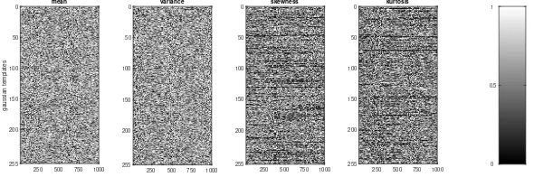
Figure 6: Leakage certification tests on simulated measurements.
We use the MATLAB source code provided by Durvaux et. al. in [dur] to perform
our leakage certification test. Specifically, we randomly generate 1000 samples from the
leakage model given in Eq. 33for each possible intermediate value and train 256 leakage
models independently. Each leakage model can be expressed as N µ,ˆ σˆ2
, the first six moments and cross validation are used. Samples with same size of validation set are randomly generated from this model. We then perform leakage certification test on them,
of which the experimental results are shown in Fig. 6. Thep-values output by our different
6
Experiments on ATMega644P Microcontroller
6.1
Measurement Setup
Our second experiment is performed on the measurements provided by Durvaux et al.
in their leakage certification code [dur]. These measurements are leaked from an AES
Furious algorithm implemented on an 8-bit Ateml AVR (ATMega644P) microcontroller.
Let z and k denote the target input plaintext byte and subkey, and y = z⊕k. For
each possible value ofy, 1000 encryptions and measurements are collected. Then, leakage
certification tests are performed on them.
6.2
Low Discretization of Leakage Samples
Compared with real leakage, measurements sampled from simulated leakage model are more random. They also have higher discretization and better satisfy the given distri-bution. Moreover, we know the specific leakage function (i.e. real leakage model) in simulation experiments. In order to compare the fitting performance between MED and real model, we can simply compare MED with leakage function. However, the real leakage model of cryptographic devices is unknown and can only be measured by other methods such as hypothesis tests.
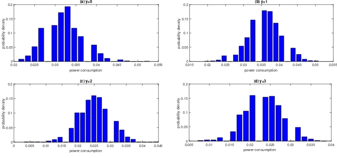
It is worth noting that the leakage samples of ATMega644P microcontroller provided
by Durvaux et al. in [dur] is with low discretization. We have tested a lot ofy-s under
all 1000 measurements and give the probability density functions corresponding to y =
0, . . . ,3 in Fig. 7. The probability density values close to the middle of distribution are 0,
but some others close to the edges are significantly high. We also carry out experiments on AT89S52 micro-controller and obtain similar conclusions. The randomness of leakage model reflected by these low discrete samples is also reduced. There could be three reasons for this phenomenon: (1) the leakage of the device is not normally distributed, (2) the size of measurements is too small, and (3) the measurement limitations of the oscilloscope.
(a) y=0
0.02 0.025 0.03 0.035 0.04 0.045 0.05 0.055 power consumption
0 0.05 0.1 0.15 0.2
probability density
(b) y=1
0.015 0.02 0.025 0.03 0.035 0.04 0.045 0.05 0.055 power consumption
0 0.05 0.1 0.15 0.2
probability density
(c) y=2
0 0.005 0.01 0.015 0.02 0.025 0.03 0.035 0.04 0.045 power consumption
0 0.05 0.1 0.15 0.2
probability density
(d) y=3
0.005 0.01 0.015 0.02 0.025 0.03 0.035 0.04 power consumption
0 0.05 0.1 0.15 0.2
probability density
Figure 7: Low data discretization of leakage from ATMega644P micro-controller.
The matrix G is close to singularity if we use Newton-Raphson method to fit MED
and true leakage distribution under the condition that the leakage samples are with low
discretization. We change the accuracy ǫ in our iteration to 10−6. It is worth noting
that, although we reduce the accuracy in our iteration in Table 3 (y=1), the number of
iterations increase compared to Table2. The algorithm needs to iterate about 16 times.
also show the experimental results of GUM tests in Table3, which indicates that the mean of these samples is about 0.0249 and the variance is about 0.0050.
Table 3: Parameters under different numbers of measurements.
measurements iteration MaxEnt GUM
ˆ
µ σˆ
200 15 5.7612 0.0247 0.0050
400 16 5.2089 0.0249 0.0051
600 16 4.6202 0.0257 0.0049
800 17 4.4929 0.0249 0.0052
1000 16 4.2925 0.0249 0.0050
6.3
Fitting Performance
We use the first six moments to analyse the measurements corresponding toy= 1. The
number of bins in histogram varies with the size of measurements used according to Eq.
32. Considering the first 200 and the first 300 measurements, hn is 9 and 11
respec-tively. Unlike Fig. 7, the new divisions do not exhibit the complex phenomenon that the probability density is almost 0 in the middle and high on both two sides, which is also amenable to MED fitness. However, the histogram shows another complex distribution
whenn = 200: the probability density is low in the middle and high on both two sides.
Obviously, normal distribution considering skewness and kurtosis is not enough to fit this distribution. To solve this, the observer can increase or decrease the number of bins, or
improve the algorithm so thatf(x) can still fit the complex distribution.
(a) MED4
0.025 0.03 0.035 0.04 0.045 0.05 power consmuption
0 0.05 0.1 0.15 0.2 0.25 0.3
probability density
iter=6 iter=7 iter=8 iter=9 iter=10 iter=11 iter=12 iter=13 iter=14
(b) MED5
0.025 0.03 0.035 0.04 0.045 0.05 power consmuption
0 0.05 0.1 0.15 0.2 0.25 0.3
probability density
iter=6 iter=7 iter=8 iter=9 iter=10 iter=11 iter=12 iter=13 iter=14 iter=15
Figure 8: MED4 and MED5 under different iterations.
Fortunately, one advantage of our MED is that it can theoretically fit complex
dis-tributions by making full use of information on arbitrary higher-order moments. f(x)
gradually fits the sample distribution in iterations under first five and six moments (see MED4 and MED5 in Fig. 8). Specifically, the irregular probability density distribution
of samples has been found after 11 iterations in our MED. f(x) shows the same
charac-teristics as the probability density distribution of samples in the twelfth iteration: low in
the middle, high on the left and low on the right. Although the errorǫ reduces, MED-s
almost coincide in the 13th, 14th and 15th iterations. It is very difficult to distinguish
them in Fig. 8(2). f(x) passes through the middle of most of bins, which shows very
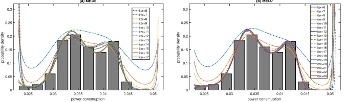
and MED5, the fitting curves of MED6 and MED7 are more complex and curved, which implies that the fitting performance is much better.
The number of iterations of MED6 and MED7 is also higher than that of MED4 and MED5 under the same accuracy. Moreover, the higher order moments fit better than the lower order moments under the same number of iterations. We also obtain similar
conclusions in Section 5.3. λin Fig. 9 and Fig. 10 changes slightly as the iteration reaches
a certain point. Maximum entropy distributions f(x) also change very little, and they
eventually overlap in the last a few iterations.
(a) MED6
0.025 0.03 0.035 0.04 0.045 0.05 power consmuption 0 0.05 0.1 0.15 0.2 0.25 0.3 probability density iter=6 iter=7 iter=8 iter=9 iter=10 iter=11 iter=12 iter=13 iter=14 iter=15 iter=16 iter=17 (b) MED7
0.025 0.03 0.035 0.04 0.045 0.05 power consmuption 0 0.05 0.1 0.15 0.2 0.25 0.3 probability density iter=6 iter=7 iter=8 iter=9 iter=10 iter=11 iter=12 iter=13 iter=14 iter=15 iter=16 iter=17 iter=18 iter=19 iter=20 iter=21 iter=22 iter=23
Figure 9: MED6 and MED7 under different iterations.
It is noteworthy that the observer is likely to obtain differentf(x) when using varying
numbers of measurements, or different measurement sets of the sample size. However,
f(x) can well reflect the true distribution of current measurements. MED represents
the most unbiased, most objective and most reasonable distribution estimation of the observed measurements. When the number of power traces increases, the observer gets
a better sample distribution and a decreasing maximum entropy (as shown in Table 3).
We also test our MED under more measurements. For example, the MED of first 300
measurements corresponding to y = 1, of which the probability follows a distribution
with left side up but the right side sloping down smoothly. Therefore,f(x) first ascends
at both ends and finally the left-end ascends to fit the high probability density while the
right-end gradually descends to fit the low probability density on the right. Finally,f(x)
fits well to the true distribution of measurements. Similar conclusions and fitting process can also be obtained from Fig. 4, Fig. 5, Fig. 8 and Fig. 9.
mean
250 500 750 1000 0 50 100 150 200 255 gaussian templates variance
250 500 750 1000 0 50 100 150 200 255 skewness
250 500 750 1000 0 50 100 150 200 255 kurtosis
250 500 750 1000 0 50 100 150 200 255 1 0.5 0
Figure 10: Leakage certification of leakage from ATMega644P Microcontroller.
Fig. 8 and Fig. 9 fully embody the super fitness ability of our MED. We use the first six moments (MED5) in our leakage certification test and obtain very good fitting performance in our leakage certification tests (as shown in Fig. 10). However, due to the pre-mentioned low data dispersion of the leakage of ATMega644P microcontroller, many
MED models cannot fit the distribution of measurements on the modelN µ,ˆ ˆσ2
the leakage certification tests (see horizontal blank lines in Fig. 10). Moreover, pvalue in Welch’s t-test is in function of the number of measurements used for certification as
stated by Durvaux et al. in [DSP16]. This also indicates that the information on the first
six moments (MED5) is insufficient to ensure thatf(x) accurately fits the distribution of
measurements. Therefore, in order to fit the distribution, we need to take information on higher-order moments into consideration. For example, the first seven or eight moments (MED6 and MED7) in Fig. 9, or even using the information on moments with orders larger than 7. We also carry out leakage certification tests on MED4, of which the results
show thatpvalues on MED5 look ’whiter’. This also shows that the fitting performance
of the higher-order moments is better.
7
Conclusion and Future Works
The accuracy of a leakage model plays a very important role in side-channel attacks and evaluations. In this paper, we aim to determine the true leakage model of a chip. To achieve this, we performed Maximum Entropy Distribution (MED) estimation on higher-order moments of measurements to approximate the true leakage model of devices rather than assume a leakage model. Then, non-linear programming is used to solve the Lagrange multipliers. The MED is the most unbiased, objective and reasonable probability density distribution estimation that is built on known moment information. It does not include the profiler’s subjective knowledge of the model. MED can well approximate the true distribution of the leakage of devices, thus reducing the model assumption error and estimation error. It can also well approximate the complex distribution (e.g. non-gaussian distribution). Both theoretical analysis and experimental results verify the feasibility of our proposed MED.
MED can theoretically use information on arbitrary higher-order moments to infinitely approximate the true distribution of leakage. In this case, more moments mean more information. However, more moments also necessitate more computation. In our future work, we will explore methods to accurately measure the amount of information on each moment and make MED choose the right moments for each iteration. We also plan to improve our MED to make it converge faster, thereby reducing the number of iterations and computation time.
References
[BCO04] Eric Brier, Christophe Clavier, and Francis Olivier. Correlation power analysis
with a leakage model. In Cryptographic Hardware and Embedded Systems
-CHES 2004: 6th International Workshop Cambridge, MA, USA, August
11-13, 2004. Proceedings, pages 16–29, 2004.
[BDGN14] Shivam Bhasin, Jean-Luc Danger, Sylvain Guilley, and Zakaria Najm. Side-channel leakage and trace compression using normalized inter-class variance.
InHASP 2014, Hardware and Architectural Support for Security and Privacy,
Minneapolis, MN, USA, June 15, 2014, pages 7:1–7:9, 2014.
[BPG18] Florian Bache, Christina Plump, and Tim Güneysu. Confident leakage
assess-ment - A side-channel evaluation framework based on confidence intervals. In 2018 Design, Automation & Test in Europe Conference & Exhibition, DATE
2018, Dresden, Germany, March 19-23, 2018, pages 1117–1122, 2018.
[CGD18] Yann Le Corre, Johann Großschädl, and Daniel Dinu. Micro-architectural
cortex-m3 processors. InConstructive Side-Channel Analysis and Secure De-sign - 9th International Workshop, COSADE 2018, Singapore, April 23-24,
2018, Proceedings, pages 82–98, 2018.
[CRR02] Suresh Chari, Josyula R. Rao, and Pankaj Rohatgi. Template attacks. In
Cryptographic Hardware and Embedded Systems - CHES 2002, 4th Interna-tional Workshop, Redwood Shores, CA, USA, August 13-15, 2002, Revised
Papers, pages 13–28, 2002.
[DCE16] A. Adam Ding, Cong Chen, and Thomas Eisenbarth. Simpler, faster, and more
robust t-test based leakage detection. InConstructive Side-Channel Analysis
and Secure Design - 7th International Workshop, COSADE 2016, Graz,
Aus-tria, April 14-15, 2016, Revised Selected Papers, pages 163–183, 2016.
[DS16] François Durvaux and François-Xavier Standaert. From improved leakage
detection to the detection of points of interests in leakage traces. InAdvances
in Cryptology - EUROCRYPT 2016 - 35th Annual International Conference on the Theory and Applications of Cryptographic Techniques, Vienna, Austria,
May 8-12, 2016, Proceedings, Part I, pages 240–262, 2016.
[DSP16] François Durvaux, François-Xavier Standaert, and Santos Merino Del Pozo.
Towards easy leakage certification. InCryptographic Hardware and Embedded
Systems - CHES 2016 - 18th International Conference, Santa Barbara, CA,
USA, August 17-19, 2016, Proceedings, pages 40–60, 2016.
[DSV14] François Durvaux, François-Xavier Standaert, and Nicolas Veyrat-Charvillon.
How to certify the leakage of a chip? In Advances in Cryptology -
EURO-CRYPT 2014 - 33rd Annual International Conference on the Theory and Ap-plications of Cryptographic Techniques, Copenhagen, Denmark, May 11-15,
2014. Proceedings, pages 459–476, 2014.
[dur] http://perso.uclouvain.be/fstandae/PUBLIS/171.zip.
[FSJL+10] Flament Florent, Guilley Sylvain, Danger Jean-Luc, Elaabid M, Maghrebi
Houssem, and Sauvage Laurent. About probability density function estimation
for side channel analysis. InConstructive Side-Channel Analysis and Secure
Design - 1st International Workshop, COSADE 2010, 2010, pages 15–23, 2010.
[GBTP08] Benedikt Gierlichs, Lejla Batina, Pim Tuyls, and Bart Preneel. Mutual
infor-mation analysis. InCryptographic Hardware and Embedded Systems - CHES
2008, 10th International Workshop, Washington, D.C., USA, August 10-13,
2008. Proceedings, pages 426–442, 2008.
[GG84] Stuart Geman and Donald Geman. Stochastic relaxation, gibbs distributions,
and the bayesian restoration of images. IEEE Trans. Pattern Anal. Mach.
Intell., 6(6):721–741, 1984.
[IO95] IEC ISO and BIPM OIML. Guide to the expression of uncertainty in
mea-surement. Geneva, Switzerland, 1995.
[Jay57] Edwin T Jaynes. Information theory and statistical mechanics.Physical review,
106(4):620, 1957.
[JS17] Anthony Journault and François-Xavier Standaert. Very high order masking:
Efficient implementation and security evaluation. InCryptographic Hardware
and Embedded Systems - CHES 2017 - 19th International Conference, Taipei,
[KJJ99] Paul C. Kocher, Joshua Jaffe, and Benjamin Jun. Differential power
analy-sis. In Advances in Cryptology - CRYPTO ’99, 19th Annual International
Cryptology Conference, Santa Barbara, California, USA, August 15-19, 1999,
Proceedings, pages 388–397, 1999.
[MD92] Ali Mohammad-Djafari. A matlab program to calculate the maximum entropy
distributions. In Maximum Entropy and Bayesian Methods, pages 221–233.
Springer, 1992.
[MOP07] Stefan Mangard, Elisabeth Oswald, and Thomas Popp.Power analysis attacks
- revealing the secrets of smart cards. Springer, 2007.
[Mor12] Amir Moradi. Statistical tools flavor side-channel collision attacks. In
Ad-vances in Cryptology - EUROCRYPT 2012 - 31st Annual International Con-ference on the Theory and Applications of Cryptographic Techniques,
Cam-bridge, UK, April 15-19, 2012. Proceedings, pages 428–445, 2012.
[MRSS18] Amir Moradi, Bastian Richter, Tobias Schneider, and François-Xavier
Stan-daert. Leakage detection with the χ2-test. In Cryptographic Hardware and
Embedded Systems - CHES 2018 - 20th International Conference, Taipei,
Tai-wan, September 25-28, 2018, Proceedings, pages 209–237, 2018.
[MS16] Amir Moradi and François-Xavier Standaert. Moments-correlating DPA. In
Proceedings of the ACM Workshop on Theory of Implementation Security,
TIS@CCS 2016 Vienna, Austria, October, 2016, pages 5–15, 2016.
[MW15] Amir Moradi and Alexander Wild. Assessment of hiding the higher-order
leakages in hardware - what are the achievements versus overheads? In
Cryptographic Hardware and Embedded Systems - CHES 2015 - 17th
Inter-national Workshop, Saint-Malo, France, September 13-16, 2015, Proceedings,
pages 453–474, 2015.
[Pee13] Eric Peeters. Advanced DPA Theory and Practice. Springer New York, 2013.
[PSDQ05] Eric Peeters, François-Xavier Standaert, Nicolas Donckers, and Jean-Jacques Quisquater. Improved higher-order side-channel attacks with FPGA
experi-ments. InCryptographic Hardware and Embedded Systems - CHES 2005, 7th
International Workshop, Edinburgh, UK, August 29 - September 1, 2005,
Pro-ceedings, pages 309–323, 2005.
[Rep16] Oscar Reparaz. Detecting flawed masking schemes with leakage detection
tests. InFast Software Encryption - 23rd International Conference, FSE 2016,
Bochum, Germany, March 20-23, 2016, Revised Selected Papers, pages 204–
222, 2016.
[RGV17] Oscar Reparaz, Benedikt Gierlichs, and Ingrid Verbauwhede. Fast leakage
assessment. InCryptographic Hardware and Embedded Systems - CHES 2017
- 19th International Conference, Taipei, Taiwan, September 25-28, 2017,
Pro-ceedings, pages 387–399, 2017.
[RO04] Christian Rechberger and Elisabeth Oswald. Practical template attacks. In
Information Security Applications, 5th International Workshop, WISA 2004,
Jeju Island, Korea, August 23-25, 2004, Revised Selected Papers, pages 440–
[RSV+11] Mathieu Renauld, François-Xavier Standaert, Nicolas Veyrat-Charvillon, Dina Kamel, and Denis Flandre. A formal study of power variability issues and
side-channel attacks for nanoscale devices. In Advances in Cryptology -
EU-ROCRYPT 2011 - 30th Annual International Conference on the Theory and Applications of Cryptographic Techniques, Tallinn, Estonia, May 15-19, 2011.
Proceedings, pages 109–128, 2011.
[Sco79] David W Scott. On optimal and data-based histograms. Biometrika,
66(3):605–610, 1979.
[SGUK08] Aladdin Shamilov, Cigdem Giriftinoglu, Ilhan Usta, and Yeliz Mert Kantar.
A new concept of relative suitability of moment function sets. Applied
Mathe-matics and Computation, 206(2):521–529, 2008.
[Sha48] Shannon. The mathematical theory of communication. Bell System Technical
Journal, 27, 1948.
[SKR00] Munirathnam Srikanth, H. K. Kesavan, and P. H. Roe. Probability density
function estimation using the minmax measure. IEEE Trans. Systems, Man,
and Cybernetics, Part C, 30(1):77–83, 2000.
[SKS09] François-Xavier Standaert, François Koeune, and Werner Schindler. How to
compare profiled side-channel attacks? In Applied Cryptography and
Net-work Security, 7th International Conference, ACNS 2009, Paris-Rocquencourt,
France, June 2-5, 2009. Proceedings, pages 485–498, 2009.
[SLP05] Werner Schindler, Kerstin Lemke, and Christof Paar. A stochastic model
for differential side channel cryptanalysis. In Cryptographic Hardware and
Embedded Systems - CHES 2005, 7th International Workshop, Edinburgh, UK,
August 29 - September 1, 2005, Proceedings, pages 30–46, 2005.
[SM15] Tobias Schneider and Amir Moradi. Leakage assessment methodology - A
clear roadmap for side-channel evaluations. In Cryptographic Hardware and
Embedded Systems - CHES 2015 - 17th International Workshop, Saint-Malo,
France, September 13-16, 2015, Proceedings, pages 495–513, 2015.
[SMY09] François-Xavier Standaert, Tal Malkin, and Moti Yung. A unified framework
for the analysis of side-channel key recovery attacks. InAdvances in Cryptology
- EUROCRYPT 2009, 28th Annual International Conference on the Theory and Applications of Cryptographic Techniques, Cologne, Germany, April
26-30, 2009. Proceedings, pages 443–461, 2009.
[SUK06] Aladdin Shamilov, Ilhan Usta, and Yeliz Mert Kantar. Performance of
max-imum entropy probability density in the case of data which are not well
dis-tributed. InProceedings of the 6th WSEAS International Conference on
Sim-ulation, Modelling and Optimization, Lisbon, Portugal, September 22 - 24,
2006, Proceedings, pages 361–364, 2006.
[Ven10] Alexandre Venelli. Efficient entropy estimation for mutual information
anal-ysis using b-splines. InInformation Security Theory and Practices. Security
and Privacy of Pervasive Systems and Smart Devices, 4th IFIP WG 11.2 In-ternational Workshop, WISTP 2010, Passau, Germany, April 12-14, 2010.
Proceedings, pages 17–30, 2010.
[Wan97] MP Wand. Data-based choice of histogram bin width. The American
[XM10] Fang Xinghua and Song Mingshun. Estimation of maximum-entropy distri-bution based on genetic algorithms in evaluation of the measurement
uncer-tainty. InIntelligent Systems (GCIS), 2010 Second WRI Global Congress on,
volume 1, pages 292–297. IEEE, 2010.
[ZH88] Arnold Zellner and Richard A Highfield. Calculation of maximum entropy
distributions and approximation of marginalposterior distributions. Journal