Enabling Query-driven Analytics via Extreme Scale In-situ Processing.

(1)

ABSTRACT

LAKSHMINARASIMHAN, SRIRAM. Enabling Query-driven Analytics via Extreme Scale In-situ Processing. (Under the direction of Nagiza F. Samatova.)

Efficient analytics of scientific data from extreme-scale simulations is quickly becoming a top-notch priority. Scientific simulations that are driven by local space-time relation-ships are largely performed with the purpose of discovering or explaining non-local and large-scale space-time relationships through interactive, query-driven, what-if data ex-ploration. The data generation process of typical simulations proceed from one time step to the next and requires the context of only two time steps, while storing data for only one time step on the disk. In contrast, data analytics often requires the full context of the available data, not just a single time step. Thus, the fundamental differences in data context and heterogeneity of access patterns demand analytics-driven data management solutions.

One promising approach for achieving these ends is in-situ processing, i.e., process-ing simulation output while the output still resides in applications’ memory. However, enabling in-situ data-analytics at extreme-scale requires a number of algorithmic chal-lenges to overcome. First, coupling analysis with simulation execution requires techniques that are non-intrusive to the simulation, while being computationally efficient and hav-ing the ability to operate in-core. This constraint renders many current state-of-the-art analytics techniques inapplicable in an in-situ context. Second, data-intensive analy-sis routines, which are predominantly query-driven, are bottlenecked on access to slow storage devices. Thus, to sustain reduced response times over extreme scale data, ana-lytics routines must breakaway from the existing practice of creating large pre-computed indexes that trade storage for computational efficiency. Third, before the simulation out-put leaves the comout-pute cluster, data must first be made analysis-ready, by aggregating across spatial/temporal resolutions. This however, needs to happen in-network, under network-bandwidth and memory constrained scenarios. Arguably, a transformative shift is necessary, making data analytics and data reduction first class citizens of the data management design and information processing.

(2)

compres-sion routine in In-situ Sort-And-B-spline Error-bounded Lossy Abatement (ISABELA) of scientific data that is unlike existing lossless compression techniques, which are hardly suitable for scientific data due to its inherently entropic nature. With ISABELA, we

apply a preconditioner to seemingly random and noisy data along spatial resolution to achieve an accurate fitting model that achieves a≥0.99 correlation with the original data while providing compression rates of ≈ 85% and introducing only a negligible overhead on simulations in terms of runtime.

To support analytics-driven efficient query processing, we build a parallel query pro-cessing engine, called ISABELA-QA. ISABELA-QA takes an orthogonal approach

when compared with the traditional indexing of raw data, by binning and generating a value-based index over _ISABELA-compressed data that results in an order of magni-tude reduction in index storage. The memory light-weight index enables a query execu-tion model that offers more than a 10-fold speed-up in per-core processing along with a multi-fold reduction in energy consumption. By turning an IO-bound problem into a compute-bound problem, we achieve a design that is inherently scalable on multi-node, multi-core, and GPU configurations.

And finally, we propose DIRAQ, a parallel in-situ, in-network data indexing and

reorganization technique that enables the transformation of simulation output into a query-efficient form, with negligible runtime overhead to the simulation run. DIRAQ

(3)

Enabling Query-driven Analytics via Extreme Scale In-situ Processing

by

Sriram Lakshminarasimhan

A dissertation submitted to the Graduate Faculty of North Carolina State University

in partial fulfillment of the requirements for the Degree of

Doctor of Philosophy

Computer Science

Raleigh, North Carolina

2013

APPROVED BY:

Xiaosong Ma Frank Mueller

Kemafor Ogan Nagiza F. Samatova

(4)

DEDICATION

In loving memory of my father, S. Lakshminarasimhan, and grandfather, G. N.

(5)

BIOGRAPHY

(6)

ACKNOWLEDGEMENTS

The successful completion of this dissertation would not have been possible without the goodwill and guidance of several people.

First and foremost, I am indebted to my advisor Nagiza Samatova for taking me under her wing and guiding me throughout my thesis study. It was her encouragement in the first place that made me convert to the Ph.D. program. Her confidence in me has on several occasions been overwhelming, but it has directly contributed to my growth as a person. Her research productivity, determination and drive have never ceased to amaze me and these characteristics have been a constant source of motivation for me to improve my own work ethic. Even with all my efforts, the primary accelerators for the timely and successful completion of this dissertation have been Nagiza’s open-door policy and round-the-clock reachability. I could go on, but keeping it short, I feel truly blessed to have an advisor like her, and, not surprisingly, her insight and guidance have extended well beyond my academic life.

I am very thankful to my committee members: Professors Xiaosong Ma, Frank Mueller and Kemafor Ogan, for their valuable support, guidance and constructive comments that have helped improve this thesis. I am grateful to Douglas Reeves for admitting me into the Ph.D. program with funding. I had the privilege to learn a great deal and derive inspiration from several professors in the department, particularly Rada Chirkova and George Rouskas.

I have learned a lot from collaborating with several experts in the field of high-performance computing: Scott Klasky, Norbert Podhorszki and Qing Liu from Oak Ridge National Laboratory and Rob Ross, Venkat Vishwanath and Rob Latham from Argonne National Laboratory. I am especially thankful to them for providing me access to lead-ership class computing resources and the necessary software infrastructure for me to work with. The summer I spent at Argonne, with Venkat Vishwanath, Mark Hereld and Michael Papka, was particularly productive, and I am grateful to them for providing such an excellent research environment. Additionally, I would like to thank Stephane Ethier, Sueng-Hoe Ku, C.S. Chang, Hemanth Kolla and Jackie Chen for providing me access to, and helping me understand the simulation datasets I have used throughout my thesis.

(7)

critique my papers and offer corrections that markedly improved the presentation of the papers. I am thankful to David (Drew) Boyuka for the work on DIRAQ. I have enjoyed innumerable long discussions with him on a wide variety of topics, which have almost always ended up being enlightening for me. Eric Schendel deserves a special mention for being the go-to guy in our group on addressing any questions regarding code optimization. I am grateful to Isha Arkatkar, Zhenhuan Gong, Xiaocheng Zou and Saurabh Pendse for assistance on various papers.

I am under immense obligation to Kanchana Padmanabhan – my confidante, counsel and closest friend for the past 4 years. Her positive attitude and patience have been a source of inspiration for me. And special thanks to her for sitting through multiple dry-runs of almost all my presentations and offering constructive criticisms and suggestions that helped me polish them. I would like to thank my friends Naga, Sairam and TC for flying in for my defense. In addition to them, I would like to thank Mohit, Ramprasad, Sandeep, Suresh, Vasanth, and Vignesh for their constant support and encouragement.

Finally, none of this would have been even remotely possible if it were not for the patience and support of my family members. My mother Chandralekha, sister Vidya and brother-in-law S.K. Rangaswamy have been pillars of strength and their sacrifices have made my Ph.D. study realizable. I would also like to express my gratitude to my relatives Ravi and Jayashree for providing me with the financial assistance that helped me get started with my graduate studies.

(8)

LIST OF TABLES

Table 2.1 Summary of GTS output data by different categories. . . 16 Table 2.2 Performance of examplar lossless and lossy data compression

meth-ods. . . 17 Table 2.3 Impact of ∆–encoding onCR for Potential (Density). . . 29 Table 2.4 ISABELAvs. Wavelets for fixed CR = 81% andW0 = 1,024. . . 30 Table 2.5 XGC data analysis showing the correlation between radial zones on

original data . . . 33 Table 2.6 Impact of error quantization on correlation between radial zones on

ISABELA-compressed data, and the difference with the correlation

over original data. . . 33 Table 2.7 Mis-classification rate for 100-iteration k-means on the Flash and

GTS datasets. Sample size is 4096 2-D points. represents the bounded error per data point. . . 35 Table 2.8 S3D Global maxima of absolute relative errors with the original

data, for mean and standard deviation across 50 timesteps for 20 million points. For mean of velocities u, v, w, we consider values >3m/s, and for standard deviation σ >1m/s. For temperature we consider values withσ >5 Kelvin (the peak variance in the domain is about 3.8E+ 05K2_{). . . .} ₃₆

(11)

LIST OF FIGURES

Figure 1.1 The scientific method cycle of today’s extreme-scale simulation ap-plications. . . 2 Figure 1.2 Components of this thesis. . . 10

Figure 2.1 A slice of GTS Potential: (A) original; (B) sorted; (C) decoded after B–splines fitting to original; and (D) decoded after B–splines fitting to sorted. . . 18 Figure 2.2 A cubic B-spline fitting with m = 6 control points, k = 10 knots,

and with 3 piecewise cubic segments. . . 20 Figure 2.3 Illustration of ∆–encoding of the index across temporal resolution. 24 Figure 2.4 Workflow of _ISABELA compression engine from data generation

toin-situ compression to storage. . . 25 Figure 2.5 Accuracy (ρ): (a) Per window correlation for Wavelets,B−splines,

and _ISABELA with fixed CR = 81% for GTS Density. (b) Per window correlation for GTS linear and non-linear stage Potential decompressed by ISABELA. . . 26

Figure 2.6 Sensitivity ofN RM SE values for_ISABELA-compressed GTS Po-tential data across 100 windows over varying window sizes. The compression rate is fixed atCR= 81.44% . . . 27 Figure 2.7 Compression ratio (CR) performance: (a) For various per point

relative error thresholds (τ) in GTS Potential during linear and non-linear stages of the simulation. (b) For various timesteps with τ = 1% at each point (for GTS Potential:t1 = 1,000, ∆t = 1,500; for Velocity in Flash:t1 = 3,000, ∆t= 3,500. . . 28 Figure 2.8 Compression ratio (CR) performance with per-window constraint

ρ >0.99, and N RM SE <0.01: (a) On each window, with varying number of coefficients, in Flash velx (b) Overall storage cost over 400 windows across various petascale simulation datasets. . . 31 Figure 2.9 Comparison of intensity plots of the normalized temperature values

in XGC data, across temporal and poloidal dimensions for original (left) and ISABELA (middle) decompressed data. The absolute

difference between the derived values, on an order of magnitude lower scale, are shown in the figure on the right. . . 32 Figure 2.10 Plot of derived turbulence intensity values over 620 timesteps across

different radial zones in XGC simulation. . . 34

(12)

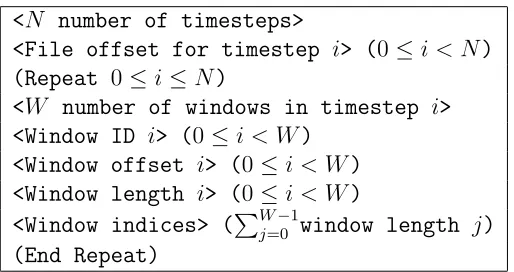
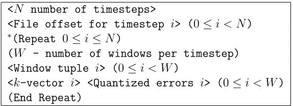
Figure 3.2 Bin-based index file format for spatial regions. . . 46 Figure 3.3 Bin-based index file formats for quantized errors. Each window

tu-ple contains the window ID, the window offset, the number of val-ues within the window in the bin, and the offset in memory of the uncompressed k-vector.∗Each section is compressed using the standard compression library zlib. . . 47 Figure 3.4 Comparison of the accuracy for GTS Potenital data for FastBit,

between quantized and raw values with level of binning. Significant relative error >1%, is relative error () of a quantized value with respect to its original value. . . 51 Figure 3.5 Precision of query results obtained onISABELA-compressed 3.2GB

GTS potential data. . . 52 Figure 3.6 Comparison of end-to-end query response times over varying

selec-tivity on data of size 1 TB. . . 53 Figure 3.7 Comparison of end-to-end region-centric query response times over

varying selectivity on data of size 32 GB. . . 54 Figure 3.8 Performance of computational components ofISABELA-QAquery

processing over varying selectivity. . . 55 Figure 3.9 Comparison of overall compute and I/O costs over varying selectivity. 56 Figure 3.10 A comparison between serial, CPU-parallelized, and GPU-parallelized

B-spline regeneration. 8 OpenMP threads were used in this particu-lar plot, corresponding to two quad core Intel Xeon X5355 processors. 57 Figure 3.11 Speedup of queries requesting spatial regions only and optionally

variables. 16 OpenMP threads are used, on four quad-core proces-sors on a single node. . . 58 Figure 3.12 Components of distributed query processing over larger (10%)

se-lectivity sizes of the 32 GB GTS data. . . 59

Figure 4.1 Overview of the DIRAQ indexing methodology, with lightweight encoding1,2_{, scalable index aggregation}8,9 _{and resource-aware} dy-namic aggregator selection 6. . . 66 Figure 4.2 An overview of how raw floating-point data is encoded by_DIRAQ

for compact storage and query-optimized access. CII stands for compressed inverted index. . . 70 Figure 4.3 A logical view of group index aggregation and writing. . . 72 Figure 4.4 Steps for building a group index layout on the leader core (shown

for a group size of 2, generalizable for more cores). . . 74 Figure 4.5 Accuracy of the performance model prediction on Group Layout,

(13)

Figure 4.6 Comparison of response times of DIRAQ compressed (CII) and un-compressed (II) indexes with FastQuery, over various aggregation sizes, on queries of fixed-selectivities. . . 82 Figure 4.7 Resulting index sizes (as a % of raw data) on varying amount of

data aggregated per-core with FastQuery (FQ) and DIRAQ (CII) indexing techniques. . . 83 Figure 4.8 Strong scaling on the effective end-to-end throughput (original data

size / end-to-end encoding time) on 3 FLASH simulation datasets indexing a total of 2 GB, on Intrepid. PFPP (POSIX file-per-process) and MPI-IO (two-phase collective) perform raw data writes with no overhead of indexing. . . 84 Figure 4.9 Weak scaling on the effective throughput (original data size /

end-to-end indexing time) for 3 FLASH simulation datasets indexing 1 MB on each core on Intrepid. PFPP, MPI-IO performs raw data writes with no overhead of indexing. . . 85 Figure 4.10 Cumulative time spent on each stage of DIRAQ for 4 datasets from

FLASH simulation on Intrepid, with each process indexing 1 MB of data using an uncompressed index (II), and a compressed inverted index (CII). . . 86 Figure 4.11 Comparison of different aggregation strategies (number of compute

(14)

Chapter 1 Introduction

Scientific simulations in the past decade have utilized the exponential growth in com-putational capabilities, effectively scaling to hundreds and thousands of processes. As a result, these simulations can now simulate physical phenomena at unprecedented level of detail, scale and can generate upto several hundreds of terabytes of data during a sin-gle simulation run. However, with increasing amounts and complexity of data produced, post-processing analysis is becoming increasingly challenging, and without a proportion-ate increase in I/O bandwidth, this problem is expected to get exacerbproportion-ated.

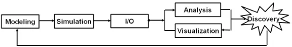
Analysis and visualization of large-scale simulation data sets place unique I/O re-quirements owing to fundamental differences in data context and access patterns among the simulation and exploratory data analytics steps (see Figure 1.1). The data generation process of space-time simulation proceeds in a local manner, from one time step to the next, and requires the context of only two time steps, while storing data for only one time step at a time on the disk. In contrast, data analysis and visualization steps often require thefull context of the available data, not just a single time step. In fact, simulations that are driven by local space-time relationships are largely performed with the purpose of discovering or explainingglobal and large-scale space-time relationships through analysis and visualization [28].

(15)

Figure 1.1: The scientific method cycle of today’s extreme-scale simulation applications.

the analysis and visualization software rely on high-performance I/O much more heav-ily than simulations in order to provide scientists with an interactive environment for the full context data exploration. However, it is a well-known phenomenon that I/O ac-cess rates have not kept pace with high-performance computing performance as a whole. For this reason, new paradigms are needed to support the unique needs of analysis and visualization for extreme-scale simulation applications, especially in the full context.

Typically, exploratory accesses over scientific datasets are made in the form of queries that involve constraints on one or more variable values. For example, a commonly used query over S3D combustion simulation [34] datasets involves identifying all regions in space at a particular timestep where 100 < uvel < 120 and constructing a probability density function or a histogram of the values satisfying the points of interest. Based on the analysis of the above output, a new query may be formulated, where either the query ranges or the variables themselves are updated. And, as this process is repeated iteratively, constant access on the entire raw output over slow devices quickly becomes inefficient.

Rather than performing a full scan of the data for each incoming query, utilizing an efficient indexing scheme can help accelerate query response times by several orders of magnitude. Indexing techniques such as bitmap indexes [6, 71] and B-Trees [18] have shown to extremely effective in a large number of scenarios involving databases and also with scientific applications [52, 74]. However, at current rates of data generation that are seen with extreme-scale simulations, the storage overhead of these indexing techniques can be more than 200% of the data being indexed. While indexes are traditionally de-signed to trade storage for computational efficiency, application scientists’ operate under environments that are constrained on both limited I/O storage and access bandwidth1_. Hence, generally, application scientists are not interested in solutions that result inmore

1_{The IBM BG/P cluster “Intrepid” at Argonne National Laboratory that is equipped with 163,840}

(16)

data [60] and, in contrast, reducing data and its movement has become a top priority at exascale.

1.1 Evolving Data Analysis Pipeline

The scientific data analyses have been evolving from a pure post-processing regime to one with a hybrid mixture of simulation-time and post-simulation form of analysis. Two main factors have influenced this change in the analysis pipeline. First, simulation-time anal-ysis elimates the need for writing the data to storage and reading it back for processing by storing the data to be analyzedin memory of analysis or compute nodes. In contrast, post-processing (processing the output after simulation completion) has become an in-creasingly tedious process, where extensive movement of terabytes and petabytes of data to and/or from storage nodes is necessary and highly expensive. Second, simulation-time processing not only allows immediate insight into the ouput, but also provides a frame-work that can equip scientists with the ability to explore data at real-time. The vision of such a framework involves feeding results of analyses back into the running simula-tions and eventually steering them [47]. [It is noted that not all analysis routines can be performed concurrently with the running simulation.] Despite an increase in the number of compute resources, the available memory is insufficient to aggregate and analyze data across a large number of timesteps. Large-scale time-series analyses will still need to be deferred till post-simulation in order to perform out-of-core processing. However, several forms of data exploration and a large class of analysis routines can take advantage of the improved compute capabilities on leadership class machines, making simulation-time analysis a reality [47, 78, 65].

(17)

DataStager [4], GLEAN [66], or PreData [80] to move the simulation output away to a set of nodes designated for data analysis. As simulations continue with their computation without much delay (provided data processing and I/O times are kept up with the rates of data generation), these staging nodes typically have to perform processing with several orders-of-magnitude less compute power and memory bandwidth. Additionally, not all simulations can easily optimize their codes to employ extra staging resources.

Even though simulation-time analysis involves almost no I/O access, query-driven exploration would still benefit from having the simulation output in a form that is read-efficient across different levels of the memory hierarchy. To perform such transformations without impacting the simulation run-time, placing the processing routines such as in-dexing, data reduction directly onto the compute nodes, i.e., using in-situ processing, can be a viable approach. There is a clear need to have the data “analysis-ready” by the time it leaves the compute cluster, and preparing the data for analysis post-simulation only delays the “time-to-analysis.”

1.1.1 In-situ

Processing for Query-driven Analytics

The primary goal ofin-situ processing is to reorganize and transform the data to make it more efficient for both real-time and post-simulation time query processing. However, the ideal data layout in memory for simulation computation does not usually translate into an efficient layout on disk for data-intensive analytics. To effectively scale across a large number of processes during computation, simulation scientists employ different levels of domain and data decomposition. The most common decomposition involves dividing the simulation into spatial regions and mapping them to processes. And within each process, arrays of variable values are further sub-divided in memory to optimize for cache and memory accesses. Storing the data as-is from each process may be efficient for writes, but the non-contiguous accessses during reads incur a large number of seeks, thereby resulting in a significant degradation in performance.

(18)

harnessed, and admits in-memory indexing, eliminating a round-trip to disk.

Designing scalable,in-situ algorithms is a challenging task and majority of the current state-of-the-art data management solutions are inapplicable in an in-situ or an extreme-scale context because of the following reasons:

1. Increase in compute capabilities largely translates to more processors and cores-per-procesor while memory-per-core and processor speeds remain at the same level. Processing data along with simulation execution mandates memory-lightweight and parallelizable solutions, while existing solutions are better suited for the post-processing phase.

2. Even as I/O bandwidth lags behind compute power by several orders of magnitude, existing solutions accelerate query-driven analysis by generating pre-computed in-dexes that can be significantly larger than the original data. As analysis operations remain highly data-intensive and require efficient out-of-core processing to scale, frequent seeks and large reads over slow storage devices result in increased response times.

3. Before the simulation output leaves the compute cluster, the data must first be made analysis-ready, by aggregating and indexing across spatial, and possibly tem-poral contexts. Such aggregation schemes must be resource-aware in order to meet network-bandwidth and memory constraints. However, with auxillary indexes that expand the data, efficientin-network aggregation and I/O in such scenarios become challenging.

The current state-of-the-art techniques are opposed to one of the central goals of in-situ computation: to minimally disturb application run time.Arguably, a transformative shift is then necessary, making data analytics and data reduction the first class citizens

of the data management design and information processing. In this thesis, we propose

(19)

1.2 Challenges with Storage-Efficient Scientific Data

Analytics

An efficient data management scheme that enables exploratory analytics, driven by in-dexing and compression, requires careful design of underlying structures for ensuring scalability. In that regard, we review some of state-of-the-art techniques in the literature that specifically relate to scientific data compresion and indexing and we identify their applicabilityin-situ.

1.2.1 Compression

Using compression to reduce the amount of data accessed from storage can be an effective strategy to address the I/O bottleneck during visualization and analysis. While there are numerous approaches for performing data reduction, we focus primarily on the following techniques that are currently in use with scientific datasets: sampling, lossless compression and lossy compression.

Random sampling is arguably the simplest of all reduction methods. It provides a viable solution for reducing the data size, while preserving some statistical properties of the data (e.g., mean, standard deviation, or density function). However, it is hardly practical for a number of reasons. On the one hand, random data sampling requires random I/O disk access that easily becomes prohibitively expensive for large-scale data sets; in fact, full sequential data scan could provide a faster, yet not practical, solution. On the other hand, features that are of interest to scientists, such as unusual, extreme or rare events, will be likely missed if only a random data sample is being used.

(20)

datasets are written once and read many times, and hence requires larger compression ratios and fast decompression for exploratory querying.

Lossy compression techniques using Discrete Cosine Transform [5], Discrete Wavelet Transform [21], or B-splines [10] discard information content for significantly higher com-pression ratios compared to lossless comcom-pression techniques. While these techniques have been proven in the field of signal processing, they offer poor approximation accuracy on many of the scientific datasets used in this thesis, as these datasets do not emanate from signal sources. This loss in accuracy could lead to interesting phenomena being missed during the analysis phase. Thus, solutions that guarantee error-bounds on every point in the approximated data become necessary to improve quality of exploratory query results, without sacrificing encoding throughput or compression ratios.

1.2.2 Indexing

Much of the pioneering work in scientific data indexing comes from the database com-munity even as traditional relational databases are not suitable for scientific datasets for a number of reasons (support for arrays, column based representation for analysis, cost, scalability etc.) [60]. However, one specific form of indexing used in databases, bitmap in-dexes, introduced in 1985 [62], have shown great promise and wide applicability. Bitmap indexes were designed to target read- or append-only attributes (variables), which aligns with the write-once read-only characteristic of most scientific simulation datasets. These bitmap indexes originally employed no compression and were shown to be effective for low cardinality attributes, i.e., the number of unique values in the variable is only a few. However, with the addition of compression, they were shown to be optimal even for high cardinality attributes [71] and have been effective in accelerating analytical processing on scientific datasets in several cases [74, 50, 52, 70].

To reduce the storage requirements of bitmap indexes on scientific datasets, past studies have focused on three main strategies: binning, encoding, and compression [63].

(21)

binning based on precision, queries can be answered approximately and quickly by using just the index. The bitmap vector for a bin for a variable consisting of N elements is then a 0/1N-bit vector, with a 1 in the corresponding element position whose value satisfies the bin condition or 0, otherwise.

• Encoding defines the relationship between bins. Each bin can represent a unique value or a non-overlapping range of values such astemp= 10.0 (equality-encoding), or an overlapping interval of values such as 5.0≤temp <10.0 (interval-encoding), or a cumulative range of values like temp ≤10.0 (range-encoding). Both interval-encoding and range-interval-encoding are ideally suited for range queries over floating-point data in terms of computational overhead, but equality encoding tends to take the lowest space requirement amongst the three and offers a good balance between space usage and query performance.

• Compression is applied on each bitmap vector by identifying runs, which are con-secutive sequences of 0’s or 1’s, and replacing the runs with a run count and a bit value. The state-of-the-art compression with bitmap indexes, the word-aligned hybrid compression (WAH) [71], takes advantage of the fact that memory accesses happen in units of words and aligns literals (sequences containing both 0’s and 1’s) and fills (compressed long runs) to word boundaries. This reduces inefficient memory accesses when operating over compressed bitmaps, and WAH is extremely efficient in performing logical operations directly in the compressed space without having to decode the bitmaps. However, enforcing this alignment improves CPU processing times during querying, increases the storage costs of bitmap indexes and hence poses a challenge in severely I/O bottlenecked environments.

(22)

analysis the query ranges and workload cannot possibly be knowna priori. A few other techniques such as data reorganization to eliminate seeks during candidate checks have also shown promise [75], but they again incur increased storage requirements.

Even with all the above improvements, the storage and encoding overhead of bitmaps makes them inapplicable as an in-situ indexing technique.

1.3 Hypothesis

Based on the challenges explained above, the central hypothesis of this thesis can be stated as follows:

Storage-efficient indexing solutions are essential for scalable indexing and query

pro-cessing for large-scale scientific simulations running on high-performance computing

en-vironments. And, utilizing in-situ processing capabilities for data compression and

cre-ation of storage-lightweight indexes can significantly reduce both the time-to-analysis and

response times for query-driven analytics.

1.4 Proposed Approaches

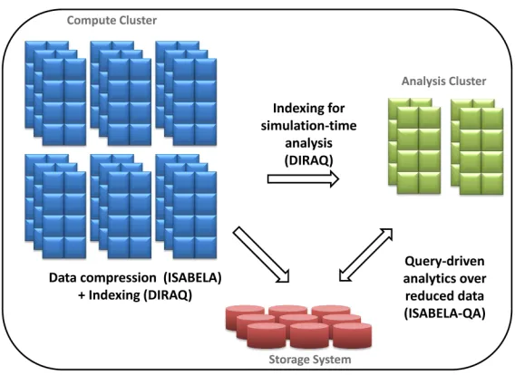
This thesis contributes new approaches that cover the complementary areas of (a)in-situ lossy data compression, (b) query-driven analytics over lossy-compressed data, and (c) parallel indexing using in-situ processing. The main components of this thesis (Figure 1.2) and the summary of their approaches and results are described below.

1.4.1 ISABELA for Effective

In-situ

Compression of Scientific

Data

We first introduce an effective lossy compression method named_ISABELA(In-situ Sort-And-B-spline Error-bounded Lossy Abatement) of scientific data [54]. The intuition be-hind ISABELA stems from the following three observations. First, while being almost

(23)

Figure 1.2: Components of this thesis.

to, their goodness of fit with significantly fewer coefficients to store. Finally, the mono-tonicity property of the sorted data gets preserved in most of its positions with respect to adjacent time steps in many instances. Hence, this property of monotonic inheritance across temporal resolution offers yet another venue for improvement of the overall data compression ratio.

While intuitively simple, ISABELA has addressed a number of technical challenges

imposed by end-user requirements. One of the most important factors for the user’s adop-tion of any lossy data reducadop-tion technology is the assurance that the user-acceptable error-bounds are respected. Since curve fitting accuracy is often data-dependent, ISABELA

must be robust in its approximation. While curve fitting operations are traditionally time consuming, performing the compressionin-situ mandates _ISABELAto be fast. Finally, while data sorting—as a pre-conditioner for data reduction—is “a blessing,” it is “a curse” at the same time; reordering the data requires keeping track of the new position indices to associate the decoded data with its original ordering. While management of spline coefficients could be viewed as a light-weight task, the heavy-weight index management forcesISABELAto make some non-trivial decisions between the data compression rates

and the data accuracy.

(24)

Not only does it consistently outperforms Wavelet transform technique, but also delivers better performance, in terms of both compression ratio and accuracy. By capturing the relative per point errors and applying error quantization,ISABELA provides over 75%

compression on data from XGC, GTS and FLASH simulation applications, while ensuring 99% accuracy on almost all values. Furthermore, several analytical operations such as correlation and query-driven processing benefit from quick approximate solutions that can be obtained by operating overISABELA-compressed data. The storage-efficient solution

over error-bounded compressed data leads to accurate results on analytical operations over XGC and GTS simulation data sets (> 99% correlation at per-point relative error = 0.1%) when compared with the original data. The ISABELA-compressed data and

its parallel storage framework are thus ideally suited for scientific data analytics and visualization routines.

This work is published in part at the 17th _{International European Conference on} Parallel and Distributed Computing (Euro-PAR 2011) [54] as a distinguished paper and the full version is published in the Journal of Computation and Concurrency: Practice and Experience [42].

1.4.2 QA: Query-driven Analytics over

ISABELA-compressed Data

We propose a parallel query processing engine, called ISABELA-QA that is designed

and optimized forknowledge priors driven analytical processing of spatio-temporal, mul-tivariate scientific data that is initially compressed,in-situby ourISABELA technology.

WithISABELA-QA, the total data storage requirement is less than 30% of the original

data, which is the eight-fold less than what the existing state-of-the-art data management technologies that require storing both the original data and the index, such as FastBit could offer. Since ISABELA-QA operates on the metadata generated by our

com-pression technology, its underlying indexing technology for efficient query processing is light-weight; namely it requires less than 3% of the original data, unlike existing database indexing approaches that require over 200% of the original data. Moreover, ISABELA-QA is specifically optimized to retrieve the actual values rather than spatial regions

(25)

offer-ing a light-weight memory and disk storage footprint solution with parallel, scalable, multi-node, multi-core, and GPU-based query processing.

This work has been published in the Conference on High Performance Computing Networking, Storage and Analysis (SuperComputing) in 2011 [41].

1.4.3 DIRAQ: Scalable Data Encoding for Analytical Query

Processing

With ISABELA and ISABELA-QA, we created an inherently lossy compression tech-nique. Based on the lessons learnt, we proposed DIRAQ [40], a parallel, scalable, in-situ index building algorithm, which creates losslessly compressed data with an inbuilt precision-based index for approximate query processing. DIRAQ aggregates group-level indexes across large spatial contexts without significantly impacting the simulation per-formance. It proceeds by first dividing the processes in the simulation into processor set (pset) groups based on network topology, and then applies in-situ indexing on each local process. The encoding technique converts raw floating-point data into a compressed rep-resentation, which incorporates a compressed inverted index to enable optimized range-query access, while also exhibiting a total storage footprint less than that of the original data. Once the indexes are built, the layout of the group-level “defragmented” index layout is created at the group-leader by communicating and merging local index layouts. A load-balanced data transfer mechanism takes place using in-network Remote Memory Access (RMA) operations, to move the index to writer nodes, which then writes the aggregated index to disk. Additionally, we introduced a new approach for aggregator selection that incorporates data-, topology- and memory-awareness to enable smarter aggregation strategies at run-time.

Our proposed method showed promising results on 9 datasets from the FLASH as-trophysics simulation [7] and 4 datasets from S3D combustion simulation [34]. Our en-coding reduced the overall storage footprint versus the raw data by a factor of 1.1 - 1.8x, and versus indexes created using FastQuery [17] (parallel version of FastBit) by 3 - 6x. Our scalable reorganization and aggregation method combined with our encoding allows up to 6x to-disk throughput improvement compared to MPI-IO on the raw data. Fi-nally, query performance on our defragmented indexes was improved by up to 10x versus FastBit-generated bitmap indexes.

(26)

Interna-tional Symposium on High-Performance and Distributed Computing Conference (HPDC

(27)

Chapter 2 ISABELA for Effective In-situ

Compression of Scientific Data

2.1 Introduction

Spatio-temporal data produced by large-scale scientific simulations easily reaches ter-abytes per run. Such data volume poses an I/O bottleneck—both while writing the data into the storage system during simulation and while reading the data back during analysis and visualization. To alleviate this bottleneck, scientists have to resort to subsampling, such as capturing the data every sth timestep. This process leads to an inherently lossy data reduction.

In-situ data processing—or processing the data in-tandem with the simulation by utilizing either the same compute nodes or the staging nodes—is emerging as a promis-ing approach to address the I/O bottleneck [46]. To complement existpromis-ing approaches, we introduce an effective method for In-situ Sort-And-B-spline Error-bounded Lossy Abatement (ISABELA) of scientific data [54]. ISABELA is particularly designed for

compressing spatio-temporal scientific data that is characterized as being inherently noisy and random-like, and thus commonly believed to be incompressible [68]. In fact, the ma-jority of the lossless compression techniques [11, 51, 56] are not only computationally intensive and therefore hardly suitable for in-situ processing, but also are only unable to reduce such data by around 10-25% of its original size (see Section 2.3).

(28)

exhibits a very strong signal-to-noise ratio due to its monotonic and smooth behavior in its sorted form. Second, prior work done in curve fitting [29, 69] has shown that mono-tone curve fitting, such as monomono-tone B-splines, can offer some attractive features for data reduction including, but not limited to, their goodness of fit with significantly fewer co-efficients to store. Finally, the monotonicity property of the sorted data gets preserved in most of its positions with respect to adjacent time steps in many instances. Hence, this property of monotonic inheritance across temporal resolution offers yet another venue for improvement of the overall data compression ratio.

While intuitively simple, ISABELA has addressed a number of technical challenges

imposed by end-user requirements. One of the most important factors for the user’s adop-tion of any lossy data reducadop-tion technology is the assurance that the user-acceptable error-bounds are respected. Since curve fitting accuracy is often data-dependent, _ISABELA must be robust in its approximation. While curve fitting operations are traditionally time consuming, performing the compressionin-situ mandates ISABELAto be fast. Finally,

while data sorting—as a pre-conditioner for data reduction—is “a blessing,” it is “a curse” at the same time; reordering the data requires keeping track of the new position indices to associate the decoded data with its original ordering. While management of spline coefficients could be viewed as a light-weight task, the heavy-weight index management forcesISABELAto make some non-trivial decisions between the data compression rates

and the data accuracy.

2.2 A Motivating Example

Much of the work forin-situ data reduction in this study stems from particle simulation codes, specifically Gyrokinetic Tokamak Simulation (GTS) [67] and XGC1 [53] which re-spectively simulate micro-turbulence of magnetically confined fusion plasmas of toroidal devices in cores and edges of fusion reactors. Production runs of these simulation appli-cations typically consume hundreds of thousands of cores on petaflop systems, such as NCCS/ORNL Jaguar [9], utilizing the ADIOS library [45] for performing I/O intensive operations.

(29)

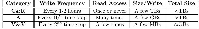
(3) diagnostics data used, for example, for code validation and verification (V&V) (see Table 2.1).

Table 2.1: Summary of GTS output data by different categories.

Category Write Frequency Read Access Size/Write Total Size

C&R Every 1-2 hours Once or never A few TBs ≈TBs

A Every 10th time step Many times A few GBs ≈TBs

V&V Every 2nd _{time step} _{A few times} _{A few MBs} _≈GBs

Unlike C&R data that requires lossless compression, analysis (A) data is inherently lossy, and as such, it can tolerate some error-bounded loss in its accuracy. What is more important is that it is the analysis data that is being accessed many times by different scientists using various analysis and visualization tools or Matlab physics analysis codes. Therefore, aggressive data compression that could enable interactive analytical data ex-ploration is of paramount concern, and is therefore the main focus of _ISABELA. For illustrative purposes, in the rest of the paper we will use linearized 64-bit double precision floating point arrays. The temporal snapshots consist of series of 172,111 values organized one-dimensionally of both Potential and Density fluctuations from GTS analysis data, a series of 4,096 values organized three-dimensionally from Flash astrophysics data, and a series of 124,701 turbulence intensity values organized one-dimensionally from XGC1 analysis data.

2.3 Problem Statement

(30)

sci-entific data often exhibits a large degree of fluctuations in values across even directly adjacent locations in the array. These fluctuations renderlossy multi-resolution compres-sion approaches like Wavelets [24] ineffective.

The compression ratio CRM(D) of a compression method M for data D of size |D| reduced to size |DM| is defined by Equation 2.1:

CRM(D) =

|D| − |DM|

|D| ×100%. (2.1)

The accuracy of lossy encoding techniques is measured using Pearson’s correlation coef-ficient (ρ) and Normalized Root Mean Square Error between anN−dimensional original data vector D= (d0, d1, . . . , dN−1) and decompressed data vectorD0 = (d00, d01, . . . , d0N−1) defined by Equations 2.2, and 2.3:

ρ(D) = covariance(D, D

0₎

std dev(D)std dev(D0₎ =

1 N

PN−1

i=0 (di −D)(d¯

0

i−D¯0) r

1 N

PN−1

i=0 (di−D)¯ 2

r 1 N

PN−1 i=0 (d

0 i−D¯0)

2

, (2.2)

where ¯D=

PN−1 i=0 di

N , and ¯D

0 ₌

PN−1 i=0 d

0 i N

N RM SEM(D) =

RM SEM(D, D0)

Range(D) =

q PN−1

i=0 (di−d0i) 2

max(D)−min(D) (2.3) Capturing both NRMSE andρprovides not only the extent of error but also measures the degree to which the original and approximated data are linearly related. Thus, achiev-ing N RM SEM(D) ∼ 0, ρ(D) ∼ 1 and CR ∼ 100% would indicate ideal performance.

Table 2.2: Performance of examplar lossless and lossy data compression methods.

Metric FPC LZMA ZIP BZ2 ISABELA Wavelets B–splines

Lossless? Yes Yes Yes Yes No No No

CRM (%) 3.12 2.72 1.13 1.11 81.44* 22.51* 0*

TC (sec.) 0.58 7.01 1.03 3.96 0.93 0.62 0.78

TD (sec.) 0.56 1.38 0.49 1.18 1.05 0.58 0.82

CRM= compression ratio of methodM,TC= compression time,TD= decompression time.

∗_CR_{achieved by lossy models for 0.99 correlation and 0.01 NRMSE fixed accuracy. All runs are performed on an Intel}

(31)

2.4 Theory & Methodology

Existing multi-resolution compression methods often work well on image data or time-varying signal data. For scientific data-intensive simulations, however, data compression across the temporal resolution requires data for many timesteps be buffered in memory, which is, obviously, not a viable option. Applying lossy compression techniques on this data across thespatial resolution requires a significant tradeoff between the compression ratio and the accuracy. Hence, to extract the best results out of the existing approxima-tion techniques, a transformaapproxima-tion of this data layout becomes necessary.

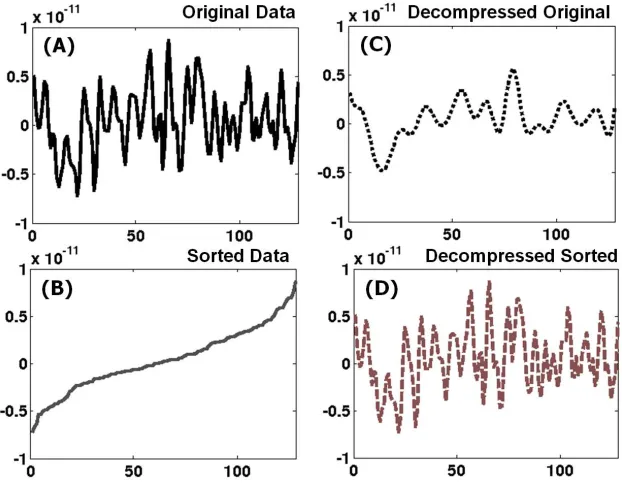
Figure 2.1: A slice of GTS Potential: (A) original; (B) sorted; (C) decoded after B– splines fitting to original; and (D) decoded after B–splines fitting to sorted.

2.4.1 Sorting-based Data Transformation

(32)

curve can provide a model that is more accurate than one on unordered and randomly distributed data. Figure 2.1 illustrates the significant contrast in how closely (D) or poorly (C) the decompressed data approximates the original data when the B−splines curve fitting [10] operates on sorted versus unsorted data, respectively.

2.4.2 Background: Cubic

B−

splines Fitting

Sorting the data in an increasing order provides a sequence of values whose rate of change is guaranteed to be the slowest. Although this sequence resembles a smooth curve, performing curve fitting using non-linear polynomial interpolation becomes difficult for complex shape curves. Computing interpolation constants for higher-order polynomials in order to fit these complex curves is computationally intensive for in-situ processing.

A more effective technique is spline curve fitting. Aspline curve is a sequence of curve segments joined together viaknots that produce a single continuous curve. Each piece of the curve segment is then defined via a lower-order polynomial function. Using several lower-order polynomial functions to fit smaller regions of the curve tends to perform highly efficiently when compared to using a higher-order polynomial function to fit the entire curve.

A B-spline curve is a sequence of piecewise parametric curves. A cubic B-spline is composed of polynomial functions of degree d = 3, which have faster interpolation time and produce “smooth” curves (i.e., second-order differentiable) at the knot locations. Knot locations are points in the parameter space that describe the start and end of a curve segment.

As an example, consider the cubicB-spline curve in Figure 2.2 with six control points, P1, . . . , P6, and ten knots, u1, . . . , u10, u1 =· · · =u4 = 0 andu7 =. . . =u10 = 1.0. The knot points are the end-points of the piecewise curve segments, S1, S2, and S3, given by S1 =sd1s2, S2 =sd2s3, and S3 =sd3s4, each defined in its parameter space, u ∈[0,1]. The control points P define the shape of the curve.

(33)

u₁= u₂= u₃= u₄= 0 u₅ u₆ u₇= u₈= u₉= u₁₀= 1 P₁

P₂ P₃

P₄

P₅

P₆

s₁

s₂

s₃

s₄

Figure 2.2: A cubic B-spline fitting with m = 6 control points, k = 10 knots, and with 3 piecewise cubic segments.

basis functions Bi,j(u) via Equation 2.4:

S(u) = m X

i=1

Bi,d(u)Pi,where (2.4)

Bi,0(u) =  



1, if ui ≤u < ui+1 0, otherwise

Bi,j(u) =

u−ui ui+j−ui

Bi,j−1(u) +

ui+j+1−u ui+j+1−ui+1

Bi+1,j−1(u), (2.5)

(34)

2.4.3 Maximizing Compression Ratio via Window Splitting

In this section, we look at approaches for maximizing the compression ratio, while main-taining an accurate approximation model. Let us assume that the original data D is a vector of size N, namely D = (d0, d1, . . . , dN−1). This way, we can associate a value di with each index valuei∈I ={0,1, . . . , N −1}. Let us also assume that each vector ele-ment, di ∈R, is stored as a 64-bit double-precision value. Therefore, storing the original

data requires |D|=N ×64 bits.

Assuming that D is a discrete approximation of some curve, its B−splines inter-polation DB requires storing only B−splines constants—the knot vector and the basis coefficients—in order to reconstruct the curve. Let C denote the number of such 64-bit double-precision constants. Then, storing the compressed data after B-splines curve fitting requires |DB|=C×64 bits.

The random-like nature ofD(see Figure 2.1, (A)) requiresC ∼N to provide accurate lossy compression, and hence, leads to a poor compression rate (see Table 2.2, last col-umn). However, due to the nature of scientific datasets, applyingB-splines interpolation after sorting D requires only a few constants, C =O(1) << N, in order to provide high decompression accuracy (see Figure 2.1, (D)).

While significantly reducing the number of B−splines constants C, sorting D will reorder the vector elements via some permutation π of its indices, namely I →π Iπ = {i1, i2, . . . , iN}, such that dij ≤dij+1,∀ij ∈ Iπ. As a result, we need to keep track of the

new index Iπ so that we could associate the decompressed sorted vector Dπ back to the original vector D by using its correct index I. Since each index value ij requires log2N bits, the total storage requirement for Iπ is |Iπ|=N×log2N bits. Therefore, the vector length N is the only factor that determines the storage requirements for the index Iπ.

One way to optimize the overall compression ratio, CR_ISABELA, is to first split the entire vector D into fixed-sized windows of size W0 (rounding up the size of the tail window for the simplicity of analysis), or D=S

Dk_,_Di_∩_Dj ₌_∅, _Ik₌_{(k₋_1)W 0,(k− 1)W0 + 1, . . . , kW0−1}, i, j, k ∈ 1, NW, i 6= j, and NW =

l N W0

m

. Then, the B−splines interpolation is applied to each windowDk _separately.

(35)

de-fined by Equation 2.6:

|D_ISABELA|= NW X

k=1

(|D_Bk|+|I_πk|), (2.6)

=NW ×(C×64 +W0×log2W0)

Substituting Equation 2.6 into Equation 2.1 and simplifying the resulting equation, we obtain the following compression ratio for _ISABELA defined by Equation 2.7:

CR_ISABELA(D) = (1−log2(W0)

64 −

C W0

)×100% (2.7)

From Equation 2.7, we can analytically deduce the trade-off between the window size W0 and the number ofB−splines constantsC that give the best compression ratio. For example, for W0 > 65,536, the size of the index alone would consume more than 25% of the original data. By fixing W0 = 1024, we balance the computational cost of sorting windows and the storage cost for recording the index and the fitting coefficients, which results in an overall compression rate of 81.4% per time step. And empirically, we found that C = 30 and W0 = 1024 allows ISABELA to achieve both > 0.99 correlation and

< 0.05 NRMSE between the original and decompressed GTS data, thus balancing for both accuracy and storage.

2.4.4 Error Quantization for Guaranteed Point-by-point

Accu-racy

The above sorting-based curve fitting model ensures accurate approximation only on aper window basis and not on aper point basis. As a result, in certain locations, theB−splines estimated data deviates from the actual by a margin exceeding a defined tolerance. For ex-ample, almost 95% of the approximated GTS Potential values average a 2% relative error, where the percentage of the relative error () at each indexibetweenD= (d0, d1, ..., dN−1) and DISABELA = (d00, d

0

1, ..., d

0

N−1) is defined as i = di−d0i

di ×100%. While the number of such location points is reasonably low due to accurate fitting achieved by B−splines on monotonic data, ISABELA guarantees that a user-specified point-by-point error is

respected by utilizing an error quantization strategy.

(36)

the data with high accuracy. Quantization of these errors into 32-bit integers results in a large degree of repetition, where majority of the values lie between [-2, 2]. These integer values lend themselves to high compression rates (75%−90%) with standard lossless compression libraries. These compressed relative errors are stored along with the index during encoding. Upon decoding, applying these relative errors ensures decompressed values to be within a user-defined threshold τ for per point relative error.

Parallel Compression

Fixing the window size, and the number of coefficients in a window keeps the compres-sion design embarassingly parallel where each window can be compressed independently. However, with the inclusion of error quantization, the size of the encoded errors and hence the size of the compressed window, no longer remains a constant. To write the compressed data into a contiguous location each thread must know a priori as to where to start writing theB−spline coefficients, index mapping and the encoded errors. This in-curs communication overhead when parallelizing the operation on a per-window level. To overcome the delay due to communication, each thread is assigned the task of compress-ing a fixed number of windows and writcompress-ing the compressed data includcompress-ing the encoded errors to a local memory space. This data is then written out to disk or passed to I/O libraries by iterating through the local memory of each thread. The number of available threads is usually limited when compared to the number of windows of data; therefore, iterating on a per-thread level incurs less overhead than moving the data around for con-tiguous I/O. In fact, placing compression routines on nodes which produce data has been shown to be effective in reducing the time taken to move data onto the disk [57]. Given that ISABELA achieves a higher degree of data reduction than the ISOBAR [56] lossless compression technique proposed by Schendel et al., further improvements in writing time can be expected.

(37)

Figure 2.3: Illustration of ∆–encoding of the index across temporal resolution.

Suppose that at timestept0, we first build the indexIπ(t0) consisting of no redundant values, which is essentially, incompressible. Hence, this index is stored as is. However, at the next timestep t0+ 1, the difference in index values ∆I+1 =Iπ(t0+ 1)−Iπ(t0) is small (see Figure 2.3) due to monotonicity of the original data values Dn_{and, hence, the} sorted values across adjacent timesteps.

Thus, instead of storing the index values at each timestep, we store the index values at t0, denoted as the reference index, along with the compressed pairwise index differences ∆I+1 between adjacent timesteps. But, in order to recover the data at time t0 +δt, we must read in both the reference index Iπ(t0) and all the first-order differences ∆I+1 between adjacent timesteps in the time window (t0, t0+δt). Therefore, the higher value of δt will adversely affect reading time. To address this problem, we instead store and compress a higher-order difference, ∆I+j =Iπ(t0+j)−Iπ(t0), where j ∈(1, δt), for the growing value ofδtuntil the size of the compressed index crosses a user-defined threshold. Once the threshold is crossed, the index for the current timestep is stored as is, and is considered as the new reference index.

2.4.6 ISABELA Data Workflow

Figure 2.4 depicts the overall data workflow behind the ISABELA compression

en-gine, starting from data generation to the organization of compressed data in storage.

ISABELA compression is characterized by a communication-free model which can be

(38)

can be extended to the I/O layer as well, thus enabling effecient data analysis. The sub-sequent section discusses some of the design considerations for each component of the workflow, along with their impacts on storage and accuracy. as is and is made the new

Figure 2.4: Workflow of _ISABELA compression engine from data generation toin-situ compression to storage.

reference index.

2.5 Results

Evaluation of a lossy compression algorithm primarily depends on the accuracy of the fitting model and the compression ratio (CR) achieved. As this compression is performed in-situ, analysis of the time taken to perform the compression assumes significance as well. Here, we evaluate ISABELA with emphasis on the aforementioned factors, using

(39)

0 0.2 0.4 0.6 0.8 1 1.2

0 20 40 60 80 100 120 140 160

Pearson corr el at ion coef fi ci ent Window Id

Wavelets B-Splines ISABELA

(a) 0.8 0.85 0.9 0.95 1 1.05

0 20 40 60 80 100 120 140 160

Pearso n correlat ion c oeffi cient Window Id Non-Linear Linear (b)

Figure 2.5: Accuracy (ρ): (a) Per window correlation for Wavelets, B−splines, and IS-ABELA with fixed CR = 81% for GTS Density. (b) Per window correlation for GTS

linear and non-linear stage Potential decompressed by ISABELA.

2.5.1 Per Window Accuracy

In this section, we compare the Pearson correlation (ρ) between the original and de-compressed data using Wavelets and B-splines on original data and using ISABELA.

The following parameters are fixed in this experiment: W0 = 1024, CB−spline = 150, and C_ISABELA= 30. This fixes CR = 81%, and wavelet coefficients values are thresholded to achieve the same compression rate as well. Figure 2.5a illustrates that ISABELA

per-forms exceptionally well even for much smaller C values due to the monotonic nature of the sorted data. In fact, ρ is>0.99 for almost all the windows. However, both Wavelets andB−splines exhibit a large degree of variation and poor accuracy across different win-dows. This translates to NRMSE values that are one-to-two orders of magnitude larger than the average 0.005 NRMSE value produced by ISABELA.

ISABELA performs exceptionally well on data from the linear stages of the GTS

(40)

2.5.2 Effect of Window Size

W

0

on Accuracy

In order to keep the compression design embarrassingly parallel, the size of the window W0 is kept fixed. The choice of window size should not only have a low index storage footprint, but must also contain sufficient number of points to approximate the curve accurately. In Figure 2.6, we calculate the N RM SE sensitivity to different values of constants C = 20,30,2×log2(W0) and to different window sizesW0 with ISABELA.

One would expect that increasingW0 without increasingC would increaseN RM SE. But this is not the case. As it turns out, the data becomes highly smooth with largerW0. Hence, N RM SE initially increases, but then it levels off as W0 keeps growing. When C = 2×log2(W0), that is the number of constants is kept constant proportional to the window size, N RM SE decreases as W grows. The choice of W = 1024 and C = 30 balances the trade-off between accuracy and compression rate, providing a fixed 81% reduction in the size of the data.

0 1 2 3 4 5 6

NR

MSE

x 0.001

Window Id

C = 20 C = 30 C = 2 log2(W0)

Figure 2.6: Sensitivity of N RM SE values for ISABELA-compressed GTS Potential

data across 100 windows over varying window sizes. The compression rate is fixed at CR= 81.44%

(41)

(a) (b)

Figure 2.7: Compression ratio (CR) performance: (a) For various per point relative error thresholds (τ) in GTS Potential during linear and non-linear stages of the simulation. (b) For various timesteps with τ = 1% at each point (for GTS Potential: t1 = 1,000, ∆t= 1,500; for Velocity in Flash: t1 = 3,000, ∆t = 3,500.

are similar when the per point relative error (τ) is fixed (see Figure 2.7a). This is because the relative error in consecutive locations for the sorted data tends to be similar. This property lends well to encoding schemes. Thus, even when the error tends to be higher in the non-linear stage, compared with the linear stage, the compression rates are highly similar. For τ = 0.1% at each point, the CR lowers to an around 67.6%. This implies that by capturing 99.9% of the original values, the data from the simulation is reduced to less than one-third of its total size.

Figure 2.7b shows the compression ratio (with τ = 1%) over the entire simulation run using the GTS fusion simulation and Flash astrophysics simulation codes. For GTS Potential data, the compression ratio remains almost the same across all stages of the simulation. With Flash, after error quantization, most relative errors are 0’s. Compressing these values results in negligible storage overhead, and henceCR remains at 80% for the majority of timesteps.

2.5.4 Effect of

∆

–encoding on Index Compression

In this section, we show that compressing along the time dimension further improves

(42)

For example, on density withW0 = 1024, the index size reduces from 15.63% to 10.63%– 13.63% with index compession. Table 2.3 show the compression rates achieved for different orders of ∆I+j, j = 1,2,3. While increasingW0 improves spatial compression to a certain extent, it severely diminishes the reduction of the index along the temporal resolution. This is due to the fact that with larger windows and a larger δt between timesteps, the difference in index values lacks the repetitiveness necessary to be compressed well by standard lossless compression libraries.

Table 2.3: Impact of ∆–encoding on CR for Potential (Density).

W0 Without ∆–encoding ∆I+1 ∆I+2 ∆I+3

512 80.08 (80.08) 81.83 (84.14) 81.87 (85.09) 81.68 (85.36)

1024 81.44 (81.44) 83.14 (85.65) 83.21 (86.57) 82.98 (86.76)

2,048 81.34 (81.34) 83.03 (85.56) 83.07 (86.44) 82.88 (86.66)

4,096 80.51 (80.51) 82.14 (84.64) 82.21 (85.51) 82.03 (85.76)

8,192 79.32 (79.32) 80.99 (83.38) 81.04 (84.24) 80.83 (84.46)

2.5.5 Compression Time

The overhead induced on the runtime of the simulation due to in-situ data compression is the net sum of the times taken to sort D, buildIπ and perform cubic B−spline fitting. However, for a fixed window size W0, sorting and building the index is computationally less expensive compared to B−spline fitting. When executed in serial, ISABELA

com-presses data at average of around 12 MB/s rate, the same as gzip compression level 6, as shown in Table 2.2. Within the context of the running simulation, if each core generates around 10 MB of data every 10 seconds, it can be reduced to ≈2 MB in 0.83 seconds using _ISABELA. Additionally, to further reduce the impact of in-situ compression on the main computation, _ISABELAcan be executed at the I/O nodes rather than at the compute nodes [3, 80].

2.5.6 Performance for Fixed Compression

In this section, we evaluate the performance of ISABELA and Wavelets on 13 public

(43)

and 7 datasets from petascale simulation applications for the fixed CR = 81%. For the Wavelet transform, we use the “fields” library package in R. To fix the compression ratio, the wavelet coeffecients with the lowest absolute values are reduced to 0. We then compare the averages ofρaandN RM SEaof ISABELA and Wavelets across 400 windows (see Table 2.4). Out of the 20 datasets, eighteen (three) datasets exhibit ρa = 0.98 with

ISABELA (Wavelets). The N RM SEa values for Wavelets are consistently an order of magnitude higher than forISABELA. Wavelets outperformISABELAonobs spitzer, which consists of a large number of piecewise linear segments for most of its windows. Cubic B−splines do not estimate well when data segments are linear.

Table 2.4: ISABELA vs. Wavelets for fixedCR = 81% and W0 = 1,024.

ρa N RM SEa

Wavelets ISABELA Wavelets ISABELA

msg sppm 0.400± 0.287 0.982 ±0.017 0.203 ±0.142 0.051 ±0.015

msg bt 0.754± 0.371 0.981 ±0.054 0.112 ±0.151 0.038 ±0.024

msg lu 0.079± 0.187 0.985 ±0.031 0.422 ±0.103 0.048 ±0.015

msg sp 0.392± 0.440 0.967 ±0.051 0.307 ±0.243 0.064 ±0.033

msg sweep3d 0.952± 0.070 0.998 ±0.006 0.075 ±0.036 0.004 ±0.003

num brain 0.994± 0.008 0.983 ±0.028 0.010 ±0.011 0.011 ±0.005

num comet 0.988± 0.018 0.994 ±0.025 0.020 ±0.020 0.010 ±0.006

num control 0.614± 0.219 0.993 ±0.017 0.083 ±0.037 0.009 ±0.002

num plasma 0.605± 0.062 0.994 ±0.004 0.277 ±0.038 0.033 ±0.004

obs error 0.278± 0.203 0.994 ±0.004 0.303 ±0.091 0.024 ±0.009

obs info 0.717± 0.136 0.993 ±0.006 0.181 ±0.078 0.026 ±0.016

obs spitzer 0.992± 0.001 0.742 ±0.004 0.005 ±0.000 0.030 ±0.000

obs temp 0.611± 0.114 0.994 ±0.011 0.096 ±0.025 0.009 ±0.003

gts phi 0.886± 0.030 0.998 ± 0.003 0.075 ±0.051 0.004 ± 0.001

gts zion 0.246± 0.024 0.996 ± 0.003 0.146 ±0.143 0.021 ± 0.009

gts zeon 0.232± 0.039 0.995 ± 0.003 0.242 ±0.063 0.018 ± 0.005

xgc iphase 0.235± 0.027 0.992 ± 0.013 0.291 ±0.012 0.022 ± 0.022

flash gamc 0.918± 0.063 0.989 ± 0.010 0.087 ±0.057 0.008 ± 0.007

flash velx 0.893± 0.055 0.999 ± 0.005 0.129 ±0.059 0.003 ± 0.002

(44)

0 10 20 30 40 50 60 70 80 90 100

0 50 100 150 200 250 300 350 400

Comp ression Ra ti o (CR) Window ID Wavelets ISABELA (a)

73.3 78.1

80.9 82.0 82.1

23.7 25.1

63.7 _61.1 69.0

0 10 20 30 40 50 60 70 80 90 100 Comp ression Ra ti o (CR) ISABELA Wavelets (b)

Figure 2.8: Compression ratio (CR) performance with per-window constraint ρ >0.99, and N RM SE < 0.01: (a) On each window, with varying number of coefficients, in Flash velx (b) Overall storage cost over 400 windows across various petascale simulation datasets.

2.5.7 Performance for Fixed Accuracy

From the end-user perspective, the input arguments are defined by accuracy levels. In this section, we evaluate the storage footprint of ISABELAunder strict accuracy constraints

of ρ > 0.99, and N RM SE < 0.01. Figure 2.8a contrasts the storage consumed by Wavelets against ISABELA, when the number of coefficients saved per window with

both methods are made flexible. In the case of _ISABELA, the compression ratio in each window remains close to the fixed values (C = 30). Even on hard-to-compress datasets like gts zion, as seen in Figure 2.8b,ISABELAoffers 3x reduction compared to Wavelets

at the same accuracy levels.

Enabling Query-driven Analytics via Extreme Scale In-situ Processing.

ABSTRACT

DEDICATION

BIOGRAPHY

ACKNOWLEDGEMENTS

TABLE OF CONTENTS

LIST OF TABLES

LIST OF FIGURES

Chapter 1

Introduction

1.1

Evolving Data Analysis Pipeline

1.1.1

In-situ

Processing for Query-driven Analytics

1.2

Challenges with Storage-Efficient Scientific Data

Analytics

1.2.1

Compression

1.2.2

Indexing

1.3

Hypothesis

1.4

Proposed Approaches

1.4.1

ISABELA for Effective

In-situ

Compression of Scientific

Data

1.4.2

QA: Query-driven Analytics over

ISABELA-compressed Data

1.4.3

DIRAQ: Scalable Data Encoding for Analytical Query

Processing

Chapter 2

ISABELA for Effective In-situ

Compression of Scientific Data

2.1

Introduction

2.2

A Motivating Example

2.3

Problem Statement

2.4

Theory & Methodology

2.4.1

Sorting-based Data Transformation

2.4.2

Background: Cubic

B−

splines Fitting

2.4.3

Maximizing Compression Ratio via Window Splitting

2.4.4

Error Quantization for Guaranteed Point-by-point

Accu-racy

2.4.6

ISABELA Data Workflow

2.5

Results

2.5.1

Per Window Accuracy

2.5.2

Effect of Window Size

W

on Accuracy

2.5.4

Effect of

∆

–encoding on Index Compression

2.5.5

Compression Time

2.5.6

Performance for Fixed Compression

2.5.7

Performance for Fixed Accuracy