Joint CFO Estimation and Data Detection in OFDM systems

(1)

University of Windsor University of Windsor

Scholarship at UWindsor

Electronic Theses and Dissertations Theses, Dissertations, and Major Papers

2017

Joint CFO Estimation and Data Detection in OFDM systems

Chunyu Mao

University of Windsor

Follow this and additional works at: https://scholar.uwindsor.ca/etd

Recommended Citation Recommended Citation

Mao, Chunyu, "Joint CFO Estimation and Data Detection in OFDM systems" (2017). Electronic Theses and Dissertations. 5910.

https://scholar.uwindsor.ca/etd/5910

This online database contains the full-text of PhD dissertations and Masters’ theses of University of Windsor students from 1954 forward. These documents are made available for personal study and research purposes only, in accordance with the Canadian Copyright Act and the Creative Commons license—CC BY-NC-ND (Attribution, Non-Commercial, No Derivative Works). Under this license, works must always be attributed to the copyright holder (original author), cannot be used for any commercial purposes, and may not be altered. Any other use would require the permission of the copyright holder. Students may inquire about withdrawing their dissertation and/or thesis from this database. For additional inquiries, please contact the repository administrator via email

(2)

Joint CFO Estimation and Data Detection in OFDM systems

by

Chunyu Mao

A Thesis

Submitted to the Faculty of Graduate Studies

through Electrical and Computer Engineering

in Partial Fulfilment of the Requirements for

the Degree of Master of Applied Science at the

University of Windsor

Windsor, Ontario, Canada

2016

c

(3)

Joint CFO Estimation and Data Detection in OFDM systems

by

Chunyu Mao

APPROVED BY:

Dr. Robin Gras School of Computer Science

Dr. Esam Adbel-Raheem

Department of Electrical and Computer Engineering

Dr. Behnam Shahrrava, Advisor

Department of Electrical and Computer Engineering

(4)

AUTHOR’S DECLARATION OF ORIGINALITY

I hereby certify that I am the sole author of this thesis and that no part of this

thesis has been published or submitted for publication.

I certify that, to the best of my knowledge, my thesis does not infringe upon

anyones copyright nor violate any proprietary rights and that any ideas, techniques,

quotations, or any other material from the work of other people included in my

thesis, published or otherwise, are fully acknowledged in accordance with the standard

referencing practices. Furthermore, to the extent that I have included copyrighted

material that surpasses the bounds of fair dealing within the meaning of the Canada

Copyright Act, I certify that I have obtained a written permission from the copyright

owner(s) to include such material(s) in my thesis and have included copies of such

copyright clearances to my appendix.

I declare that this is a true copy of my thesis, including any final revisions, as

approved by my thesis committee and the Graduate Studies office, and that this thesis

(5)

ABSTRACT

Orthogonal frequency division multiplexing (OFDM) is a multicarrier modulation

technique that is widely used in wireless broadband communication systems. The

spectral efficiency of OFDM is very high since the subcarriers are spaced as closely as

possible while maintaining orthogonality. However, one of the major problems with

OFDM that can cause performance degradation is carrier frequency offset (CFO)

which impairs the orthogonality among OFDM subcarriers, as a consequence, results

in inter-subcarrier interference.

In this thesis, an iterative algorithm for joint CFO estimation and data detection

in OFDM systems over frequency selective channels is proposed. The proposed

algo-rithm is performing both CFO estimation and data detection in the frequency domain

based on the Expectation-Maximization (EM) algorithm. The proposed algorithm

can achieve the same bit-error-rate (BER) performance as that of its time-domain

counterpart with much lower complexity.

Simulation results show that the proposed algorithm can converge after three

(6)

DEDICATION

To my parents, Huibin Mao and Yukun Wang, for their selfless contribution to

(7)

ACKNOWLEDGEMENTS

I would like to thank my supervisor Dr. Behnam Shahrrava, professor of the

department of Electrical and Computer Engineering at University of Windsor first.

The door to Prof. Shahrrava office was always open whenever I ran into a trouble

spot or had a question about my research. He consistently allowed this thesis to be

my own work, but steered me in the right direction whenever he thought I needed it.

I would also like to appreciate my thesis committee members Dr. Robin Gras

and Dr. Esam Adbel-Raheem. Without their passionate participation and input, the

thesis could not have been successfully conducted. I also want to thank Dr. Shervin

Erfani for his guidance of my research.

I would also like to acknowledge my uncle Dr. Yingming Zhao and my aunt Li

Wang for their support. They encourage me to chase my dream without any heisitate,

and I am gratefully indebted to their very valuable comments on my life.

Finally, I must express my very profound gratitude to my parents for providing

me with financial support and continuous encouragement throughout my years of

study and through the process of researching and writing this thesis. I would also

express my appreciate to my colleagues and friends, Siyu Zhang, Huyuan Li, Lin Li,

Pengzhao Song, Peibo Zhao, Akilan Thangarajah for their support and help. This

accomplishment would not have been possible without them. At last, I would like to

extend my gratitude to University of Windsor. Thank you.

(8)

LIST OF TABLES

(12)

LIST OF FIGURES

1.1 Multicarriers . . . 3

1.2 Orthogonal Subcarriers . . . 3

1.3 Doppler Effect . . . 5

1.4 CFO Effect . . . 5

1.5 Different Approachs . . . 7

2.1 Block Diagram of OFDM system . . . 12

2.2 4-PSK . . . 13

2.3 16-QAM . . . 13

3.1 The Wireless Channel . . . 17

3.2 Characterization of the Wireless Channel . . . 20

4.1 EM Algorithm Procedure . . . 36

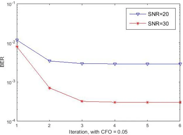
7.1 Convergence of the proposed algorithm . . . 53

7.2 BER with CFO=0 . . . 54

7.3 BER with CFO=0.03 . . . 54

7.4 BER with CFO=0.05 . . . 55

(13)

LIST OF ACRONYMS

AWGN Additive White Gaussian Noise

BER Bit Error Rate

BLUE Best Linear Unbiased Estimator

CDMA Code Division Multiple Access

CFO Carrier Frequency Offset

CIR Channel Impulse Response

CP Cyclic Prefix

CRLB Cramer-Rao Lower Bound

DFT Discrete Fourier Transform

E-step Expectation Step

EM Expectation Maximization

ICI Intercarrier Interference

IDFT Inverse Discrete Fourier Transform

ISI Intersymbol Interference

LMMSE Linear Minimum Mean Squared Error

LS Least Squares

LTI Linear Time Invariant

LTV Linear Time-Varying

(14)

MAP Maximum A Posteriori

MC Multicarrier

ML Maximmum Likelihood

MVU Minimum Variance Unbiased

OFDM Orthogonal Frequency Division Multiplexing

PAPR Peak to Average Power

PDF Probability Density Function

PSK Phase shift Keying

RBLS Rao-Blackwell-Lehmann-Scheffe

TDMA Time Division Multiple Access

WCDMA Wideband Code Division Multiple Access

(15)

1 Introduction

For the past centuries, people desire to communicate with each other in a convenience

and economical way. Due to this demand, communications has been a vibrant field

of research for more than hundred years. Thanks to the development of Very Large

Scale Integration (VLSI) and Signal Processing technology since the 1960s, wireless

communications has become one of the most significant research areas in the field

of modern communications, [1]. A tremendous advantage of wireless communication

compared with wired communication is that it does not require any physical cables.

This superiority not only enables devices to work anywhere without considering the

limitation of the wires but also saves the money.

1.1 Wireless Communications and OFDM Technique

1.1.1 The Development of OFDM Technique

In modern society, wireless communication has various excellent applications, such as

smart buildings, telecommunication, process industry, etc. As the technology

devel-opment, several techniques have been developed for wireless communication, such as

Time Division Multiple Access (TDMA), Code Division Multiple Access (CDMA),

Wideband Code Division Multiple Access (WCDMA), etc. Currently, Orthogonal

Frequency Division Multiplexing (OFDM) is the most popular multicarrier

band-efficient physical layer technique for wireless communication [2]. Multicarrier (MC)

modulation technique was first developed by Chang [3] in 1966. Todays OFDM was

introduced by Weistein and Ebert [4] in 1971, which is a special form of MC

trans-mission. In 1985, Crmini first applied OFDM in mobile wireless communication [5].

After these years development, OFDM is the most recognized technique in wireless

communication. It has various popular applications, such as digital audio

(16)

telecommunication.

1.1.2 The Advantages of OFDM Technique

OFDM has several outstanding advantages in compared with other techniques [6].

First of all, frequency domain modulation is easy to deal with the physical channel

without complex time domain equalization. Secondly, OFDM can be implemented

efficiently by using Fast Fourier Transform (FFT). Moreover, OFDM has not only

low sensitivity to time synchronization errors but also easy to integrate with

multi-antenna systems. Furthermore, intersymbol interference (ISI) can be simply handled

by adding the cyclic prefix (CP). An essential feature of OFDM [7] is that it employs

multiple narrowband orthogonal subcarriers. Due to this feature, not only the

avail-able spectrum can be used efficiently but also intercarrier interference (ICI) can be

completely eliminated. At last, this kind of subcarriers can preserve a high

trans-mission speed. Because of the above advantages, OFDM has become an excellent

technique for wireless communication.

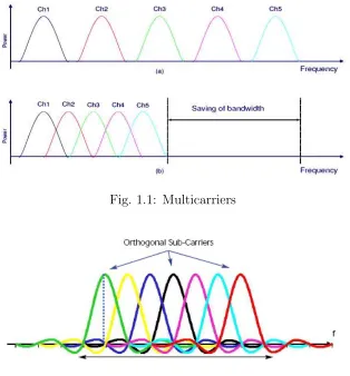
The essential characteristic of OFDM system is that it employs orthogonal

sub-carriers. In a conventional frequency division multiplexing (FDM), to eliminate ICI,

the subcarriers are spaced apart by inserting guard bands between them in the

fre-quency domain, as shown in Fig. 1.1a. However, this kind of arraignment for the

subcarriers wastes bandwidth. An alternative method is to overlap the subcarriers

to save the bandwidth as shown in Fig. 1.1b. But overlapping the subcarriers could

introduce ICI. Thus, to save bandwidth without having ICI, orthogonal subcarriers

are the best choice. OFDM is the technique that employs orthogonal subcarriers to

transmit the data. Figure 1.2 shows that the OFDM subcarriers exhibit

orthogonal-ity on a symbol interval if they are spaced in the frequency domain exactly at the

reciprocal of the symbol interval, which can be accomplished by utilizing the discrete

(17)

Fig. 1.1: Multicarriers

Fig. 1.2: Orthogonal Subcarriers

1.2 Challenges of OFDM

Nonetheless, due to the imperfect channel condition, OFDM still has several

limita-tions that would affect the performance of the system. First, in practice, a wireless

channel cannot be considered as an ideal channel [1]. As a result, the received signal is

not the same as the transmitted signal. Thus the data need to be recovered according

to the actual channel. Also, an OFDM signal can have a large peak-to-average-power

ratio (PAPR) value with high probability [8]. Moreover, strict frequency

synchro-nization is impossible to OFDM system [9] which is related to carrier frequency offset

(CFO). Furthermore, both CP and null guard tones at the edge of the spectrum can

decrease the spectral efficiency of the system. However, this thesis will focus only on

(18)

When considering the performance of a wireless communication system, the bit

error rate (BER) plays an essential role. The probability of bit error, also called,

the BER is a measure of deterioration in digital communications. Lower BER means

higher performance. In OFDM systems, due to the characteristics of the physical

channel, the BER is highly related to both parameters estimation and data

detec-tion. Generally speaking, the parameters contain timing error, channel information

and carrier frequency offset (CFO). These parameters are independent of each other.

Since the OFDM system is not sensitive to timing error [10], and the channel can be

estimated accurately by inserting a set of known symbols, called pilots, [11]. Hence,

the performance of the system is slightly affected by these two parameters. However,

the CFO cannot be easily estimated by using the pilots. The CFO is the

normal-ized frequency error between the transmitter and the receiver. In practical OFDM

systems, the CFO can be caused by the mismatch between the oscillator in the

trans-mitter and the receiver or the Doppler shift in frequency selective channels, [12]. In

practical mobile communication systems, the channel is a frequency selective

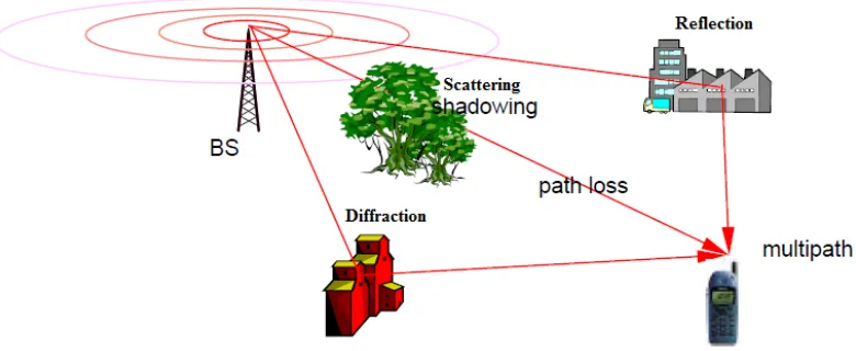
chan-nel. The details of communication channels will be given in Chapter 3. Fig. 1.3

shows how the Doppler shift leads to a frequency error. As seen in, in OFDM

sys-tems, the existence of CFO destroys the orthogonality among OFDM subcarriers, as

a consequence, results in inter-subcarrier interference [13]. And this inter-subcarrier

interference can cause BER performance degradation. As seen from Fig. 1.4, OFDM

is very sensitive to CFO [14], even a small CFO in an OFDM system can lead to a

(19)

Fig. 1.3: Doppler Effect

Fig. 1.4: CFO Effect

1.3 Research Background on CFO effect

In the literature, the CFO in an OFDM signal is modeled as a multiplicative

expo-nential function of time in the received signal in the time domain. Thus, if the CFO

can be estimated accurately, its impact can be simply eliminated by multiplying the

received symbol in the time domain with the following factor

e

(20)

which will be explained in Chapter 2. As a result, the problem is leading to how to

accurately estimate the CFO. In [12], the CFO was divided into two parts: integer

part and fractional part. The integer part does not cause inter-subcarrier interference

and only introduces a cyclic shift of data subcarriers. The integer part of CFO can

be estimated accurately by using the pilots. However, the fractional part can cause

interference among subcarriers, which results in destroying the orthogonality of the

subcarriers. The OFDM system is extremely sensitive to the fractional part of the

CFO. Since the fractional part of the CFO cannot be estimated with high accuracy

by using pilots.

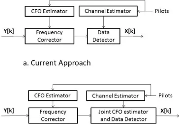
Since CFO is a key issue of OFDM systems, thus there has been numerous

re-searches on how to estimate the CFO and how to compensate it. The current approach

in the literature is to estimate the CFO first, and then correct the frequency of the

received signal based on the estimated CFO. At last, the transmitted data is being

detected based on the assumption that there is no CFO in the system. The drawback

of this approach is that an accurate estimate of the CFO cannot be obtained and

any estimation error in the CFO estimate can affect the accuracy of data detection.

As a result, if the data is detected with the assumption that the frequency

synchro-nization is perfect, then the would be larger than the real one, which means decrease

the performance of the system. From [15], current techniques prefer to estimate the

CFO by exploiting the pilots, which is called pilots-aided CFO estimation. And then

detect the data without considering the impact of CFO. In this chapter, an overview

of both current and a novel approach for CFO estimation and data detection is being

presented. Figure 1.5 shows the differences between these two approaches.

1.3.1 Current Approach

Most of current CFO estimation algorithms are based on the pilots inserted either

(21)

preamble blocks in compared to the known symbols inserted in the selected subcarrier

of the OFDM system in the frequency domain. These pilots need to be designed

carefully to increase the accuracy of the CFO estimation.

In [16], with pilots are in the time domain, a Maximum Likelihood (ML) algorithm

was developed for CFO estimation. The algorithm exploited repeated data symbols

to track the CFO by exploring the relation between the repeated blocks. The author

in [17] extends this idea by using one specified training sequence to estimate the

CFO. Furthermore, an improved CFO estimation algorithm was proposed in [18], by

redesigning the training symbols, to increase the accuracy at the expense of increasing

computational complexity.

Fig. 1.5: Different Approachs

(22)

data in the frequency domain. An estimation algorithm based on this approach,

which had two stages, was presented in [19]. Considering the performance of the

CFO estimation algorithm, pilots needed to be designed carefully. The author in [20]

proposed two novel methods to design the pilots. In [21], another method to design

pilots was presented.

The accuracy of the CFO estimation can be improved by exploiting the statistical

information about the wireless channel. A pilot-aided CFO estimator based on the

ML algorithm has been proposed in [22], and the estimation range can be improved

without decreasing accuracy [23]. By taking the channel error into consideration, two

simple methods were proposed in [24]. A joint ML-based CFO and channel estimation

algorithm was developed in [25] that has excellent performance on accuracy but with

a relatively high computational complexity.

Figure 1.5a shows that after frequency correction, the data would be detected

without considering the estimation error associated with the CFO estimate. There

are four different detection algorithms. Specifically, zero forcing (ZF) equalizer, least

squares (LS) equalizer, maximum likelihood (ML) detector, and expectation

maxi-mization (EM) detector.

ZF and LS are the algorithms based only on the transmitted symbols, the received

symbols, and the estimated channel impulse response (CIR), [26]- [27]. The ZF

equalizer is a single-tap frequency-domain linear equalizer [26]. This type of equalizer,

proposed by Robert Lucky, is simply set to the inverse of the channel frequency

response, and it can be applied to the received symbols to recover the transmitted

symbols. The term zero-forcing means when there is no noise in the system, the

ISI will be equal to zero. Based on that condition, the estimated symbols with

perfect channel information can be equal to the transmitted symbols. The idea of

ZF is simple, but it works well when the ISI is significant compared to the noise.

(23)

the modulated transmitted symbols and the received symbols. From this aspect, LS

cannot eliminate the ISI. However, the total power of noise can be minimized by this

algorithm.

In addition to the ZF and LS equalizers, the ML and EM detectors take advantage

of the statistical information of the channel estimation. The ML detector is an

al-gorithm that estimates the data symbols by maximizing the likelihood function [28].

The ML algorithm can be easily implemented compared with the EM algorithm.

However, one of the major problems with the ML detector is that it requires that

both the pilot symbols and the data symbols are equipowered. The simulation

re-sults show that the ML detector performs better than the other three detectors, [28].

However, the ML algorithm as a sequence detector in fading channels typically has

prohibitive computational complexity. The EM algorithm can be used an iterative

method for finding ML or maximum a posterior (MAP), which can be applied for

data detection in OFDM systems[29]. There are two steps for EM algorithms which

are being called Expectation and Maximization.

1.3.2 Novel Approach

Due to the limitation of the accuracy of pilot-aided CFO estimation, the novel

ap-proach, shown in Fig. 1.5b is employed for improving the accuracy of CFO estimate.

Even after the frequency corrector, the estimation error associated with CFO

esti-mate must be taken into consideration while performing data detection. There are a

few researches on the idea of joint CFO estimation and data detection.

In [30], an algorithm was proposed for joint CFO estimation and data detection

based on pilots in OFDM systems. The algorithm employs linear approximation to

present the system function and then obtains the approximated function by going

through a linear search method, such as those in [31] and [32]. Then, to reduce the

(24)

data detector. That algorithm requires linear approximation and pilots information.

However, this technique highly depends not only on the pilots, which reduce the

spec-tral efficiency of the system but also the accuracy of the pilot estimator. In [33, 34],

another algorithm for performing joint estimation that was based on a linear search

method was proposed. In each iteration, the parameters were updated based on the

minimum mean-squared error (MMSE) criterion. Moreover, in [35], an iterative

EM-based algorithm that still separately performed CFO estimation and data detection

was designed. In [36], the EM algorithm was employed for joint estimate CFO and

detect data in the time domain for OFDM systems over frequency selective fast

fad-ing channel. However, there were two major problems with this algorithm. First,

the computational complexity of the algorithm was extremely high due to the matrix

inversion and partial eigendecomposition. Second, the frequency shift in fast fading

channel cannot be separated as a constant from the channel impulse response. In

ad-dition, the frequency selective fast fading channel can only happen in high mobility,

such as avionic communications. In most cases, frequency selectivity and fast fading

cannot happen at the same time as it will be explained in Chapter 2. Thus, in most

mobile communication systems, channels are frequency selective. Hence, the idea of

jointly CFO estimation and data detection by using an iterative EM algorithm for

OFDM systems over frequency selective channels is stimulated by this research.

1.4 Objectives of the Thesis

Motivated by the issues mentioned in the section above, the objectives of this thesis

are stated as follows:

• Considering the novel approach for OFDM systems to solve the problem caused

by CFO.

(25)

• Comparing the performance of the proposed algorithm with those of the

con-ventional algorithms.

1.5 Organization of the Thesis

This thesis is mainly focused on reducing the effect of CFO on the performance

of the OFDM systems over frequency selective channels. The rest of this thesis is

organized as follows. Chapter 2 gives a background of the basic structure of OFDM

systems. Chapter 3 presents an introduction of the wireless channel. Chapter 4 gives

an overview of the algorithms related to estimation theory. Also, the

expectation-maximization (EM) algorithm, which is related to the proposed algorithm, will be

introduced in chapter 4. In chapter 5, a joint CFO estimation and data detection

algorithm in the time domain is presented. In chapter 6, a joint CFO estimation and

data detection algorithm in the frequency domain is proposed. Simulation results

and analysis are presented in chapter 7. A summary of the results abstained in this

research and suggestions for further studies are given in Chapter 8. The relevant

(26)

2 OFDM Structure

In this chapter, first, the basic structure of an OFDM system is introduced. Then, the

signal transmission procedure is stated from the mathematical point of view. Beyond

this, the effect of CFO on the transmitted signal is presented in the second part of

this chapter.

2.1 The Basis of OFDM system

Fig. 2.1: Block Diagram of OFDM system

In an OFDM system, there are mainly two components, transmitter and receiver.

Each component has several steps to process the signal in order to properly transmit

the data from the transmitter to the receiver. Fig. 2.1 illustrates is a block diagram

of a typical OFDM communication system.

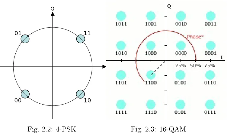
The source data are a sequence of binary bits, for example, 11100100. The

incom-ing bit stream of 1s and 0s is multiplexed into N parallel bit streams. Then, the N

parallel bit stream are independently mapped in the frequency domain into complex

symbols, denoted by X[k], in a given constellations such as phase shift Keying (PSK)

(27)

Fig. 2.2: 4-PSK Fig. 2.3: 16-QAM

PSK is a digital modulation scheme that transfers the source data by modulating

the phase of the carrier (or subcarriers), which uses a finite number of phases, each

assigned to a unique pattern of data bits. Usually, each phase encodes an equal

number of bits. Each pattern of bits forms the symbol that is represented by the

particular phase. Fig. 2.2 shows the constellation diagram for 4-PSK modulation.

QAM is another digital modulation scheme that transfers source data by

modu-lating the phase and amplitude at the same time. QAM arranges the source data in a

square grid with equal vertical and horizontal spacing, each constellating point within

the grid represent a set of bits. The constellation diagram for 16-QAM is shown in

Fig. 2.3.

Moreover, the Discrete Fourier Transform (DFT) is an essential tool for a

DFT-based OFDM system since the orthogonality of its subcarriers is preserved by the

DFT. The DFT and Inverse Discrete Fourier Transform (IDFT) are being used to

transfer the data between the time domain and the frequency domain. In an OFDM

system, ISI caused by a time-dispersive channel can be eliminated by adding a cyclic

prefix (CP) as a guard interval to a block of OFDM signal. The length of the CP

(28)

copied from the last part of each OFDM symbol block after the IDFT operation and

then it is appended to the beginning of the block. Finally, the receiver can completely

eliminate ISI by discarding the samples of the CP part before the DFT operation, as

shown in Fig. 2.1.

A mathematical expression for an OFDM signal is derived in this section. The

carrier modulated signal for an OFDM signal with a block of N symbols can be

expressed in the following complex envelope form

s(t) = Re{s˜(t)ej2πfct_} _{for 0}_≤_t _≤_{N T}

s (1)

where the complex envelope ˜s(t) can be written in the following form

˜ s(t) =

N−1

X

n=0

IDFT{X[k]}p(t−nTs), (2)

and p(t) which is known as the baseband pulse shape, may, for example, be a simple

unit-energy rectangular pulse of duration Ts, or it could be a raised-cosine pulse, a

bandlimited pulse, etc. Computing the N-point IDFT of {X[k]} gives a

complex-valued sequence {x[n]} as

x[n] = IDFT{X[k]}= 1 N

N−1

X

k=0

X[k]ej2πnk/N, n= 0,1, . . . , N −1. (3)

For convenience the following notation is used:

xn(t) =x[n]p(t−nTs). (4)

Now the OFDM signal given in (1) can be written as follows:

s(t) = Re{s˜(t)ej2πfct_}_{= Re}_{

N−1

X

n=0

(29)

or

s(t) = Re{s˜(t)}cos(2πfct)−Im{s˜(t)}sin(2πfct) (6)

= N−1

X

n=0

Re{xn(t)}cos(2πfct)− N−1

X

n=0

Im{xn(t)}sin(2πfct) (7)

At the receiver part, in an ideal communication system, which means a system with

perfect time and frequency synchronization, an ideal channel, and with no additive

noise, the received signal r(t) and the transmitted signal s(t) are identical. After all

the operations are shown in Fig. 2.1, it can be easily shown that the detected symbols

y[n] and the transmitted symbolsx[n] are equal.

2.2 The Basis of CFO Effect in OFDM system

In this section, the effect of CFO on the received signal under perfect channel condition

is investigated from a mathematical point of view. The demodulation operation at

the receiver is performed by multiplying the received signal r(t) by the signal of the

local oscillator as follows:

z(t) = ˜s(t)ej2πfct_·_ej2πfrt ₍₈₎

where fr is the frequency of the local oscillator. In order to show the CFO caused

by the mismatch between the oscillator in the transmitter and that in the receiver,

or the Doppler shift in the channel, the frequency of the local oscillator is written as

follows:

fr =fc+ ∆f (9)

where ∆f represents the CFO in the system. Then, the output signal of the

demod-ulator after lowpass filtering is given by

(30)

or

y(t) = N−1

X

n=0

xn(t)ej2π∆f t, (11)

Finally, after sampling y(t) at sampling rate Ts, the received symbol in the time

domain can be obtained as follows:

y[n] =x[n]·e

j2π∆f n

fs ₍₁₂₎

where fs is the sampling rate and ∆f

fs

is called normalized CFO (or just CFO for

simplicity).

As seen in Equation (12), the effect of CFO in the system appears as a phase error

between the transmitted symbol and the received symbol. Also, if the CFO can be

accurately estimated, the impact of CFO on the received symbol in the time domain

can be completely eliminated. This can be simply done by multiplying y[n] by the

correction factor e−j2π∆f n/fs_{, which is the reciprocal of the exponential term in Eq.}

(31)

3 The Wireless Channel

Fig. 3.1: The Wireless Channel

As mentioned in the 1st chapter, the key advantage of wireless communication

com-pared with wireline communication is that the former one has no limitation on the

communication channel. For wireline communication, the channel is a fixed

envi-ronment which means that the channel would stay constant for a relatively long

time. However, in wireless communication, the signal is transmitted via

electromag-netic waves. Due to the variation of the wave paths and the mobility of both the

transmitter and the receiver, the wireless channel becomes a significant factor to the

communication system. Figure 3.1 is a typical diagram of the wireless channel. In this

chapter, the fundamentals of the wireless channel are presented first, and then

focus-ing on the channel model in OFDM system. Current channel estimation techniques

are stated in the last section of this chapter.

3.1 Fundamentals of the Wireless Channel

Since the power of the radio waves is affected by the physical phenomenon of the

environment. Thus the environment lays the foundation of the wireless channel.

(32)

fading [38].

Large scale fading represents the average signal power attenuation due to path loss

and shadowing. More specially, path loss means the strength of the radio wave decay

with respect to a function of distance. As the distance goes longer, the power of the

wave becomes lower. In addition, even if two receivers have the same distance with the

transmitter, they may still receive a different signal due to the shadowing. Shadowing

is related to the environment between the transmitter and the receiver. Specifically,

the shadowing effect caused by obstacles in the signal paths. In most cases, this

fading effect can be accurately modeled as a random variable [39]. Fortunately, both

path loss and shadowing are typically frequency independent and could be modeled

properly. However, small scale fading does depend on the frequency which would

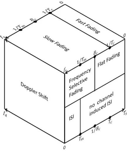
severely decrease the performance the communication system.

Small scale fading is caused not only by the constructive and destructive

interfer-ence of the different signal paths from the transmitter to the receiver which is being

called multipath propagation but also by the mobility. Considering multipath

propa-gation first, because of the different lengths of individual paths, each path would suffer

different delays, which also termed as time shift or time spread. If the maximum time

spread is greater than the symbol time, then ISI would be introduced by the channel.

Under this condition, the received symbol combines two or more transmitted

sym-bols which leading to difficulty in data detection. Otherwise, if all the spreads are

within the symbol time, then the channel induced ISI would not occur. Since time

spread in the time domain is equal to frequency selective in the frequency domain.

Thus the wireless channel under multipath propagation effect could be characterized

as frequency selective fading channel and frequency non-selective (flat) fading

chan-nel. Flat means all the subcarriers would suffer almost the same distortion. The

frequency selectivity is related to the symbol rate and channel coherence bandwidth

(33)

If the symbol rate is greater than the channel coherence bandwidth, the channel

would be frequency selective fading channel. Otherwise, the channel would be a flat

fading channel. Furthermore, there is a relation between the multipath delay and

the channel coherence bandwidth. In most wireless communication, such as mobile

communication, the channel is frequency selective channel which is being interested

in this thesis.

Moreover, if both the transmitter and the receiver are moving, then the Doppler

Effect and time variation of the channel need to be taken into consideration. The

author in [38] proves that the Doppler Effect caused by the motion leads to a spectral

compression or dilation, which is also called frequency shift. The frequency shift is

related to both the moving speed of the terminal and the carrier frequency.

Fur-thermore, due to the motion of the terminals, the propagation paths would change

all the time. This effect makes the channel as a time-varying system from nature.

Under both Doppler effect and time variation conditions, the wireless channel can

be characterized as slow fading channel and fast fading channel with respect to the

symbol time and the channel coherence time. The channel coherence time shows how

rapidly a fading channel changes with time. The fast fading channel is corresponding

to the channel with channel coherence time less than the symbol interval. For fast

fading channel, the channel is modeled as a linear time varying system which both

contain the Doppler shift and time-varying channel impulse response. The slow

fad-ing channel is used to described the channel with the channel coherence time greater

than the symbol duration. The slow fading channel can be approximately modeled

as a linear time-invariant system with frequency shift within each symbol interval.

Under this model, the frequency shift can be characterized as CFO. In most wireless

communication, the channel is slow fading channel.

From above analysis, it has been figured out that multipath propagation leading

(34)

time-varying channel impulse response. It is desired to transmitted signal in flat slow

fading channel in order to make the transmission efficient. Thus the symbol time

should be greater than the maximum multipath time spread regarding the frequency

selectivity, and smaller than the channel coherence time with respect to the time

variation. In mobile communication, the channel coherence time is much larger than

the multipath time spread (milliseconds compared to microsecond or nanosecond). As

a result, frequency selective fading and fast fading could not happen at the same time

in relative low mobility wireless communication. But for avionic communication, both

frequency selectivity and fast fading can appear at the same time. Both of the model

of frequency selective fast fading channel and frequency selective slow fading channel

would be derived in this thesis. Figure 3.2 is the block diagram of characterization

of the wireless channel in relative low mobility.

(35)

3.2 The Wireless Channel and System Model in OFDM

The last section shows that the wireless channel is an LTV system with frequency

selectivity due to the multipath propagation and moving transmitter and receiver.

One important advantage of OFDM system is that it converts a frequency selective

fading channel into flat fading channel by transmitting high-speed data to low speed

data stream via multicarrier technique. Thus the channel induced ISI is avoided, but

the signal distortion still there.

Since the effect of frequency selectivity is overcome by the multicarrier technique

in OFDM system, then only fast fading and slow fading should be considered. For

fast fading channel, the channel is modeled as an LTV system which both contain the

Doppler effect and the time-varying path propagation. One important assumption

for most of the communication system is that the major noise is at the receiver

and independent of the channel. Under this assumption, the noise is modeled as an

Additive White Gaussian Noise (AWGN). Then the relation between the transmitted

signal and received signal can be presented as

r (t) = h (t)∗s (t) + w (t)

=

∞

Z

−∞

h (t, τ) s (τ)dτ+ w (t) (13)

where s (t) is the transmitted signal, r (t) is the received signal, h (t) is the channel

impulse response, w (t) is the AWGN.

If this equation is properly sampled, then the system model in discrete form would

be

r [n] = h [n]∗s [n] + w [n]

=

∞

X

m=−∞

(36)

After removing the CP, equation (14) can be expressed in matrix form as

y=CIR(h)x+w (15)

wherey[n] is the received symbols,x[n] is the transmitted symbols, and the channel

coefficients matrix is as follow

CIR(h) =

           

h(0,0) 0 . . . h(0,2) h(0,1)

h(1,1) h(1,0) . . . h(1,3) h(1,2) ..

. ... . . . ... ...

0 0 . . . h(N −2,0) 0

0 0 . . . h(N −1,1) h(N −1,0)

            (16)

This channel is a frequency selective fast fading channel. However, this kind of

channel is only for high mobility, like avionic communication. In most cases, the

transmitter and receiver are not moving that fast, under this situation, the channel

is modeled as a Linear Time Invariant (LTI) system with frequency shift within each

symbol interval.

Alternatively, for an LTI system, the relation would change to

r (t) = h (t)∗s (t) + w (t)

=

∞

Z

−∞

h (t−τ) s (τ)dτ+ w (t) (17)

After sampling equation (17), the system model would be

r [n] = h [n]∗s [n] + w [n]

=

∞

X

m=−∞

(37)

After removing the CP, equation (18) can be expressed as

y=H(h)x+w (19)

where

H(h) =

           

h(0) 0 . . . h(2) h(1)

h(1) h(0) . . . h(3) h(2) ..

. ... . . . ... ...

0 0 . . . h(0) 0

0 0 . . . h(1) h(0)

            (20)

Now, considering frequency shift to the system, then system in time domain can

be modeled as

y=T()H(h)x+w (21)

where T=diag

h

1, e−j2Nπ, . . . , e−

j2π(N−1)

N

iT

is the CFO effect matrix.

The channel model in the above equation is called frequency selective slow fading

channel, short for frequency selective channel. Note that, for OFDM system, the

frequency shift is not only coming from Doppler effect, but also from the difference of

the oscillator between the transmitter and the receiver. The effect of frequency shift

which is termed as CFO which has already been proved in the 2nd chapter.

The corresponding frequency domain system model would be

Y =FT()H(h)x+W

=FT(ε)F−1HX+W (22)

where Y= [Y0, . . . , YN−1]T is the frequency domain received symbols and X=

[X0, . . . , XN−1]T is the frequency domain transmitted symbols, and F is theN ×N

(38)

the channel frequency response diagonal matrix and also H = diag{FLh}, where

h= [h (0), . . . ,h (L−1)]T stands for CIR vector while L is the length of channel.

Since in most applications, the system is not under high mobility, thus the

fre-quency selective channel is more adaptive. This thesis would only consider the CFO

effect in OFDM system over frequency selective channel. There is two statistic model

of frequency selective channel: Rician fading channel and Rayleigh fading channel.

If the channel has a fixed light of sight, then the CIR have a Rician distribution.

Otherwise, the CIR follows Rayleigh distribution. Since in most cases, the light of

sight is not possible, thus Rayleigh fading channel model is being used in this thesis.

3.3 Techniques of Channel Estimation in OFDM

Before properly detecting the data, the channel should be estimated first. In an

OFDM system, pilot-aided channel estimation is the most popular used technique.

The pilots can be either inserted in time domain as a preamble or in frequency domain

[40, 41, 42]. Two key factors that affect the performance of the pilot-aided channel

estimation are pilot design and interpolation. There have many researches on

pi-lots design related problems. The author in [43] proposes an algorithm to estimate

the channel by using pilot tones. The optimal design of pilots has been researched

for frequency selective channel in [44] and [45]. An overview of pilot-aided channel

estimation for wireless communication has been presented in [46]. The accuracy of

channel estimation can be improved by involving channel statistic information [42].

This thesis would focus on joint CFO estimation and data detection for OFDM

system over frequency selective channel. Thus perfect channel information is assumed

to be achieved as a prior. In addition, in order to perform joint estimation, the

estimation algorithm should be considered. In next chapter, a review of estimation

algorithms would be given. And the joint estimation algorithm would be picked based

(39)

4 Estimation Algorithms

As a result from previous chapters, it is desired to design a joint estimation algorithm

to deal with the CFO effect for an OFDM system with frequency selective channel.

From the previous chapters, we can see that the system model which both

consid-ering the CFO and the transmitted data is a linear complex matrix equation with

nonlinear parameters. Although it is extremely difficult to jointly solve this kind of

problem, there are still several algorithms that can be considered to deal with it. In

the following paragraphs, the estimation theory and associated algorithms would be

reviewed first. Then based on the comparison of the presented algorithms, the EM

algorithm would be picked to deal with the joint estimation problem and explained

in the second part of this chapter.

4.1 Review of Estimation Algorithms

Estimation can be found in many signal processing systems which designed to extract

the desired information, such as Speech, Communication, Control, etc. In order to

properly estimate the parameters, various algorithms had been developed to handle

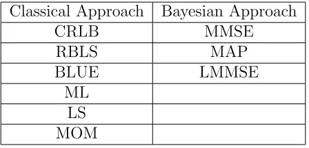
the estimation problem. Based on the characteristic of the unknown parameters, there

are two approaches: classical approach and Bayesian approach [47]. Specifically, in

classical approach, the unknown parameter is assumed to be a deterministic constant

which means the probability density function (PDF) of the parameter is not available,

and the observed data information is summarized by the PDF that depends on the

parameter. In contrast, in Bayesian approach, the unknown parameter is modeled

as a stochastic process, and the PDF of it is known as a prior. According to this

(40)

Table 4.1: Classification Of Estimation Algorithm

Classical Approach Bayesian Approach CRLB MMSE

RBLS MAP BLUE LMMSE

ML LS MOM

Since the problem that being interested is to estimate parameter vector based

on an observed data vector, which means a discrete estimation problem, then we

start with a general discrete estimation problem. After that, the algorithm is picked

by both considering the conditions and comparing different algorithms. From the

mathematical point of view, the problem is modeled as follow:

Y =S(X) +W (23)

whereYis the observed data vector,Xis the unknown parameter vector that need to

be estimated,W is the AWGN vector in most cases, but in general, it does not have

to be white Gaussian noise,S(·) represents a general transformation on the unknown

parameter.

Based on above information, the estimation problem is to derive a solution as

ˆ

X =f(Y) (24)

where ˆX is the estimated parameters, f(·) is a specified operation on the observed

data. Moreover, since the noise is modeled as AWGN, then the conditional PDF of

the observed data p(Y|X) is available.

(41)

Minimum Mean Squared Error, Maximum A Posteriori, and Linear Minimum Mean

Squared Error, respectively. Since all of these algorithms require statistic information

of the unknown parameter X as a prior, nonetheless the CFO and data are actually

deterministic without the required prior information. As a result, Bayesian approach

is not suitable for the joint estimation problem in this thesis. The algorithm for joint

estimation should be selected from the classical approach.

For classical approach, a good estimator of unknown parameters is to see whether

the average of the estimated value yields the true value and whether the variance

has the minimum value. If the average is equal to the true value, EnXˆo = X, the

estimator is called unbias estimator. And if the variance is minimized, V arnXˆo =

V armin

n

ˆ

Xo, the estimator is called minimum variance estimator. Thus the goal in

classical approach is to find a minimum variance unbiased (MVU) estimator. Based

on this criteria, several algorithms are reviewed as follows.

4.1.1 Cramer-Rao Lower Bound

First of all, Cramer-Rao Lower Bound (CRLB) is the easiest method to determine

the lower bound of the variance of any unbiased estimator. Then the estimator can

be found according to the first derivative of the ln conditional PDF.

It first assumes that

E

∂lnp(Y|X) ∂X

=0 (25)

Then the varince of the estimator would satisfy

V ar

∂lnp(Y|X) ∂X

≥ 1

−Eh∂2ln_∂p2(_XY|X)

i (26)

Then if the first derivative of the ln conditional PDF can be expressed as

∂lnp(Y|X)

(42)

As a result, X would be estimated as

ˆ

X=g(Y) (28)

From equation (28), CRLB is a straightforward method to estimate the parameters

under MVU condition. However, for nonlinear transformation as CFO, the derivative

can not be achieved easily. And even if the derivative can be achieved, the specified

expression would be a problem. Thus CRLB is not appropriate.

4.1.2 Rao-Blackwell-Lehmann-Scheffe

Moreover, Rao-Blackwell-Lehmann-Scheffe (RBLS) is another MVU estimator. By

factorizing the conditional PDF in the following form

p(Y|X) = g(T (Y),X)h(Y) (29)

The estimator can be found as

ˆ

X=k(T (Y)) (30)

where k(T(Y)) is a function that satisfy E{k(T (Y))} = Y, and T (Y) is called

sufficient statistic.

The process of finding the estimator is simple. Nevertheless, it is hard to find

the sufficient statistic and factor the PDF in the required form. Thus RBLS is not

suitable either.

4.1.3 Best Linear Unbiased Estimatore

In addition, Best Linear Unbiased Estimator (BLUE) is a suboptimal MVU estimator

(43)

that if

S(X) =HX (31)

where H is a known matrix, which means Y is linearly related to X. Moreover, the

noise has zero mean and known covariance matrix as C. Then the estimator would

be

ˆ

X= HTC−1H−1HTC−1Y (32)

Since complete PDF of the observed data Y is not necessary, BLUE is more

suitable for practical implementation. However, a key issue of BLUE is that it requires

the system has a linear relation which can not be satisfied because of the CFO as

equation (22). Thus BLUE is also not appropriate.

4.1.4 Least Squared

Furthermore, LS estimator is a basic algorithm that only minimizes the squared error.

It does not need any statistic information. The estimated parameter is the value that

minimizes the squared error function, where the squared error function is

J(X) = (Y−S(X))T (Y−S(X)) (33)

But the drawbacks are that it is neither an MVU estimator nor optimal in general.

Moreover, the direct solution is not available. Thus this algorithm is not proper to

be chosen to perform the joint estimation.

4.1.5 Method of Moments

Besides that, Method of Moments is another algorthm that do not need entire PDF of

the observed data. It only requires theN moments of the observed data Y, where N

(44)

as

ˆ

X =h−1(ˆµ) (34)

where ˆµi = _N1 PN_n₌₀Xi[n]

The advantage of this method is that it is easy to implement. However, due to

the none optimality and the requirement of multiple moments, it can not be selected

as the joint estimation algorithm.

4.1.6 Maximum Likelihood

At last, ML estimator would be the one that being chosen to solve the problem that

mentioned in the 1st chapter because of the advantages specified in the following

paragraph.

Compared with above algorithms, ML has several advantages. First of all, ML is

an optimal algorithm if the MVU estimator exists. If not, it is the approximate MVU

estimator. Moreover, it can be implemented for complicated estimation problem.

Lastly, the only requirement of it is the PDF of the observed data. Due to these

reasons, almost all practical estimators are based on the ML principle. Thus ML is

being selected at the beginning. The idea of ML is simple, the unknown parameter

X is merely the value that maximize the likelihood function p(Y|X). However, due

to the nonlinearity of the parameters in our system model, the direct form of ML

estimator can not be solved easily. Then alternative algorithms are being considered

to solve the ML problem.

Firstly, since the ML can always be found for a given data set numerically, thus

grid search is the safest method. However, considering the huge computation problem,

grid search is not a suitable solution. Under this condition, we are forced to consider

the iterative procedure. The Newton-Raphson method and the scoring approach are

two iterative methods that had been considered. Nonetheless, the convergence of these

(45)

[48], is being considered as the algorithm to maximize the likelihood function.

In comparing with the mentioned algorithms in the last paragraph, EM algorithm

is a better choice since it can maximize the likelihood function in an iterative way

with guaranteed convergence. Then the problem can be solved iteratively by treating

the observations as incomplete data. In addition, the EM algorithm does not require

any approximation and pilots information in solving the CFO problem. At last, the

EM algorithm is excellent also because of its computation simplicity. Due to above

advantages, EM algorithm is being picked to jointly estimate the CFO and detect the

data for OFDM system with frequency selective channel in this thesis. In the following

paragraphs, more details would be given to help understand the EM algorithm.

4.2 Expectation Maximization Algorithm

As stated in the last chapter, EM algorithm is a better method to solve ML detection

problem. Let’s start from ML algorithm.

Suppose that the PDF of a random known vector Y is given as f(Y|X), where

X is the vector of interest. Then the given conditional PDF of Y is the likelihood

function for ML algorithm. As a result, the solution of the ML algorithm in this

condition would be the X that maximize the likelihood function or log likelihood

function. However, if the likelihood function f(Y|X) highly nonlinear depends on

any parameters or variables, then analytical solution would not be easy to derive.

Alternatively, if there exist another random vector H which can not be observed

directly but has a relation withX, then according to Leibiz Integral Rule, we have:

f(Y|X) =

Z

f(Y,H|X)dH (35)

Under this condition, the ML problem convert to maximize the integral of the

(46)

H is called missing data, {Y,H} is called complete data.

By using Bayes’ rule, we have

f(Y,H|X) =f(H|Y,X)f(Y|X) (36)

To proceed, take the log to equation (36) and rearrange the equation, then

logf(Y|X) = logf(Y,H|X)−logf(H|Y,X) (37)

Assume we have the conditional PDF of H conditioned on Y and Xi, where Xi

represents the estimated X in the ith iteration. Then take expectation with respect

toH in equation (37) on both sides, we have

EH{logf(Y|X)} = EH{logf(Y,H|X)} −EH{logf(H|Y,X)}

=

Z

logf(Y,H|X)f H|Y,XidH

− Z

logf(H|Y,X)f H|Y,XidH (38)

Since f(Y|X) is nothing do with H, then

EH{logf(Y|X)}= logf(Y|X) (39)

Combining equation (38) and (39), we have

logf(Y|X) =

Z

logf(Y,H|X)·f H|Y,XidH− Z

logf(H|Y,X)·f H|Y,XidH

(40)

(47)

For simplicity, define

QX|Xi=

Z

logf(Y,H|X)·f H|Y,XidH (41)

P X|Xi =

Z

logf(H|Y,X)·f H|Y,XidH (42)

In order to increase the value of logf(Y|X) in each iteration, we should ensure

that

logf Y|Xi+1≥logf Y|Xi (43)

which means

Q Xi+1|Xi−P Xi+1|X1≥Q Xi|Xi−P Xi|Xi (44)

Notice that

P Xi|Xi−P Xi+1|Xi =

Z

logf H|Y,Xi·f H|Y,XidH

− Z

logf H|Y,Xi+1·f H|Y,XidH

= − Z

f H|Y,Xi·logf H|Y,X i+1

f H|Y,Xi dH (45)

Since for natural logarithm inequality, logx≤x−1whenx≥0, then

Z

f H|Y,Xi·logf H|Y,X i+1

f H|Y,Xi dH ≤ Z

f H|Y,Xi· f H|Y,X i+1

f H|Y,Xi −1 !

dH

=

Z

f H|Y,Xi+1dH− Z

f H|Y,XidH

= 1−1 = 0 (46)

Thus

(48)

for any X.

Then according to equation (44), what we need to do is to find Xi+1 that satisfies

Q Xi+1|Xi≥Q Xi|Xi (48)

By performing this operation, the Q function increases iteration by iteration,

which means iteratively maximize the likelihood function.

The method introduced above is called EM algorithm, since it constructs an

ex-pectation function first, and then maximizing the exex-pectation function iteration by

iteration. There are two steps which are called Expectation Step (E-step) and

Max-imization Step (M-step). The E-step is used to handle the randomness of some

parameters. Then the solution can be searched through maximizing the function

de-rived in E-step. In the following paragraphs, in order to give a clear idea of how the

EM algorithm works, the algorithm would be introduced via solving a simple linear

model.

Considering a general linear model as:

Y =H(h)X+W (49)

where Y is a known column vector, h is a column vector that can not be observed,

but independent of any other parameters and follow a specified distribution, such as

Gaussian Distribution. Moreover, H is nonlinear depend on h. And X stands for a

column vector need to be estimated. W is the AWGN column vector.

X should be estimated by using the above knowledge. The solution of the ML

estimate of X is

X=argmaxf(Y|X) (50)

(49)

ML estimate would not be solved easily. At this point, the EM algorithm is being

introduced to solve this problem in a relatively easy way. Within EM algorithm, Y

is called incomplete data, h is called the missing data, and {Y,h}is called complete

data. Then the likelihood function can be expressed as the integration of the marginal

likelihood function as

f(Y|X) =

Z

f(Y,h|X)dh (51)

Then ML estimation can be simplified by using the marginal PDF. The solution of

the EM algorithm is the variables that maximize the expectation of the log marginal

likelihood function as follow

X =argmaxEh

logf Y,h|Xi |Y,Xi−1 (52)

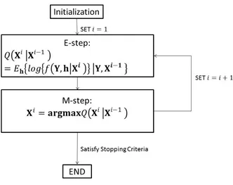
There are two iterative steps to solve this problem:

E-step:

Forming the Q function as

Q Xi|Xi−1

=Eh

log

f Y,h|Xi |Y,Xi−1 (53)

M-step:

Solving the Qfunction to find the solution at current iteration as

X =argmaxQ( Xi|Xi−1 (54)

(50)

Fig. 4.1: EM Algorithm Procedure

From this chapter, we would have a clear idea about how the EM algorithm

derived and the procedure of the algorithm. It is obvious that this algorithm is a

better choice for those systems with nonlinear parameters or variables that can not

be solved directly via ML algorithm. However, although the algorithm is simple

which only involves two steps in each iteration, the mathematical derivation for an

individual case is not as simple as the procedure. In next chapter, the EM algorithm

would be applied to an OFDM system with frequency selective channel to jointly

(51)

5 Joint CFO Estimation and Data Detection

Al-gorithm for Time Domain

In this chapter, a joint CFO estimation and data detection algorithm for OFDM

system over frequency selective channel is presented based on EM algorithm. As I

mentioned before, this joint algorithm is proposed in [36] which deal with frequency

selective fast fading channel. However, for fast fading channel, the Doppler shift can

not be characterized as CFO as described in [36]. Thus the method is not correct

in that paper. But in this thesis, the EM algorithm is being applied to frequency

selective channel which is appropriate as explained in chapter 3, and the requirement

of the pilot information is eliminated for computation simplicity. The time domain

system model is derived in chapter 3 as equation (21). The details would be given in

the following paragraphs.

The time domain OFDM system can be modeled as follow:

y=TH(h)x+w (55)

where T = diag

h

1, e−j2Nπ, . . . , e−

j2π(N−1)

N

iT

represents the matrix of CFO, y =

[y0, . . . , yN−1]T is the time domain received symbols and x = [x0, . . . , xN−1]T is the

time domain transmitted symbols with the size of N, w is the AWGN matrix with

the covariance σ2_nIN. Thus the received symbol vector y follows Complex Gaussian

distribution with mean TH(h)x and covariance matrix σ2_nIN as

f(y|x,h, ) = 1 πN_σ2

n exp

(

−(y−TH(h)x) H

(y−TH(h)x) σ2

n

)

(52)

H(h) is theN ×N convolution matrix, h= [h (0), . . . ,h (L−1)]T is the CIR and

H(h) =

           

h(0) 0 . . . h(2) h(1)

h(1) h(0) . . . h(3) h(2) ..

. ... . . . ... ...

0 0 . . . h(0) 0

0 0 . . . h(1) h(0)

            (57)

Since H(h)xrepresents the convolution, then the following property hold:

H(h)x=D(x)h (58)

where

D(x) =

           

x0 xN−1 . . . xN−L+2 xN−L+1

x1 x0 . . . xN−L+3 xN−L+2

..

. ... . . . ... ...

xN−2 xN−3 . . . xN−L xN−L−1

xN−1 xN−2 . . . xN−L+1 xN−L

            (59)

For the ML algorithm,the joint marginal likelihood function would be maximized

as

(x, ) = argmaxf(y|x, ) (60)

However the direct solution for the marginal likelihood cannot be found. Thus it

is desired to use EM algorithm to iteratively maximize the likelihood function.

The Rayleigh fading channel with covariance matrix R is being used as

p(h) = 1

πL_det_Rexp

(53)

By using Bayes’ rule

f(y,h|x, ) = f(y|x,h, )p(h|x, )

= f(y|x,h, )p(h) (62)

Now the solution of equation (60) can be found iteratively through EM algorithm

as follows.

E-step:

log{f(y,h|x, )}= log{f(y|x,h, )}+ logp{(h)} (63)

Putting equation (56) and (61) into equation (63), and dropping the terms

indepen-dent of xand

log{f(y|x,h, )} ∝log{f(y|x,h, )}

= log

(

1 πN_σ2

n exp

(

−(y−TH(h)x) H

(y−TH(h)x) σ2 n )) = log 1 πN_σ2

n

−(y−TH(h)x) H

(y−TH(h)x) σ2

n

= log

1 πN_σ2

n

−yy

H ₋_2Re

yH_TH₍_h₎_x ₊_xH_H₍_h₎H_TH_TH₍_h₎_x σ2

n

= log

1 πN_σ2

n −yy H σ2 n + 2Re

yH_TH₍_h₎_x ₋_xH_H₍_h₎H

H(h)x σ2

n

= log

1 πN_σ2

n −yy H σ2 n + 2Re

yH_TD₍_x₎_h ₋_hH_D₍_x₎H

D(x)h σ2

n

= log

1 πN_σ2

n −yy H σ2 n +

2ReyH_TD₍_x₎_h ₋_Trn_D₍_x₎H

D(x)hhHo σ2

n

∝2ReyHTD(x)h −Tr

n

D(x)HD(x)hhH o

(54)

Then the expectation of the joint log likelihood function is

Q xi, i = Eh

logf y,h|xi, i |y,xi−1, i−1

= 2Re

yHTD xi

E

h|y,xi−1, i−1

−TrnD xiHD xiEhhH|y,xi−1, i−1 o

(65)

In order to simplify the above euqation, make

µ µ

µ=E{h|y,xi−1_,i−1_} ₍₆₆₎

cov=En(h−µµµ) (h−µµµ)H|y,xi−1_,i−1o ₍₆₇₎

Then

EhHh|y,xi−1, i−1 =cov+µµµµµµH (68)

Now, equation (65) can be expressed as

Q(xi_,i_{) = 2Re}

yHTD xi

µµµ −TrnD xiH

D xi

cov+µµµµµµHo

= 2ReyHTD xiµµµ −µµµHD xiHD xiµµµ−TrnD xiHD xicovo

(69)

Based on eigen-decomposition

cov=XβffH (70)

where β is the mth eigenvalue of cov, f is the corresponding eigenvector, then

TrnD(xi₎H_D₍_xi₎_covo _{= Tr}n_{D x}iH

D xi XβffHo

(55)

Then equation (69) would be changed to

Q xi, i|xi−1, i−1 = 2ReyHTD xiµµµ −µµµHD xiHD xiµµµ

−XβfHD xiH

D xi f

= 2ReyHTD xiµµµ

−xiHH(µµµ)HH(µµµ)xi−XβxiHH(f)HH(f)xi

(72)

M-step:

In M-step, Q(xi, i|xi−1, i−1) in equation (69) is maximized with respect toxand

. Dropping those terms independent of xand .

xi, i = argmaxQ xi, i|xi−1, i−1

= argmax2ReyHTD xiµµµ

−xiHH(µµµ)HH(µµµ)xi−XβxiHH(f)HH(f)xio (73)

By setting the first derivative of argmaxQ(xi_,i−1_|_xi−1_,i−1_{) in equation (72) with}

respect to xto zero,x maximizing the function in the ith iteration as

ˆ

xi ₌_argmax_Q _xi_,i−1_|

xi−1, i−1

=hH(µµµ)HH(µµµ) +XβH(f)HH(f)i

−1

H(µµµ)HTHy (74)

Then demapping this continues data to discrete data according to the constellation

algorithm, then the estimated symbols in the ith iteration are

xi =F−1·DemappingnFxˆio ₍₇₅₎

(56)

conditional mean and conditional correlation matrix. Both of them are derived in

Appendix A as follows

µ

µµ= R−1+aH_b−1

a−1aH_b−1

y (76)

cov= R−1+aH_b−1

a−1 (77)

For the ith CFO, it can be estimated by using thexi as

i = argmaxQ xi, i|xi−1, i−1

= argmax n

2ReyHTD xiµµµ −xiHH(µµµ)HH(µµµ)xi

−XβxiHH(f)H H(f)xio (78)

Since is only a real number, then only one dimension numerical search is required

to get i _{that maximize the} _Q _{function. Then repeat the E-step and M-step until}

satisfy the stopping criteria.

Convergence is a key issue for an iterative algorithm. For the above algorithm,

the convergence can be proof.

Since

Q xi, i−1|xi−1, i−1

≥ Q xi−1, i−1|xi−1, i−1

(79)

Q xi, i|xi−1, i−1 ≥ Q xi, i−1|xi−1, i−1 (80)

Then

Q xi, i|xi−1, i−1≥Q xi−1, i−1|xi−1, i−1 (81)

The Q function is decreased iteration by iteration. Thus the convergence of this

algorithm is proved.

(57)

Initialization:

At the beginning, simply setting0 _{= 0. Then the system model reduce to normal}

linear model without CFO as

y=H(h)x+w (82)

Using LS data detector with the help of the estimated channel to have the initial

x0 _as

x0 =F−1 |H|2−1

HHY (83)

F−1 represents the IDFT. Hand Y is the corresponding frequency domain CIR and

received symbols, respectively.

Then compute in each iteration:

µ

µµ= R−1+aH_b−1

a−1aH_b−1

y (84)

cov= R−1+aHb−1a−1 (85)

Based on eigen-decomposition, we have

cov=XβffH (86)

Then

ˆ

xi ₌ h_H₍_µ_µ_µ₎H _H₍_µ_µ_µ_{) +}X_β_H₍_f₎H_H₍_f₎i

−1

H(µµµ)HTHy (87)

xi = F−1·DemappingnFxˆio ₍₈₈₎

i = argmaxn2Re

yHTD xi

µ

µµ −xiHH(µµµ)HH(µµµ)xi

−XβxiHH(f)HH(f)xio (89)

Joint CFO Estimation and Data Detection in OFDM systems

Scholarship at UWindsor

Scholarship at UWindsor

Joint CFO Estimation and Data Detection in OFDM systems

Joint CFO Estimation and Data Detection in OFDM systems

Joint CFO Estimation and Data Detection in OFDM systems

by

Chunyu Mao

A Thesis

Submitted to the Faculty of Graduate Studies

through Electrical and Computer Engineering

in Partial Fulfilment of the Requirements for

the Degree of Master of Applied Science at the

University of Windsor

Windsor, Ontario, Canada

2016

c

Joint CFO Estimation and Data Detection in OFDM systems

AUTHOR’S DECLARATION OF ORIGINALITY

ABSTRACT

DEDICATION

ACKNOWLEDGEMENTS

TABLE OF CONTENTS

LIST OF TABLES

LIST OF FIGURES

LIST OF ACRONYMS

1

Introduction

1.1

Wireless Communications and OFDM Technique

1.2

Challenges of OFDM

1.3

Research Background on CFO effect

1.4

Objectives of the Thesis

1.5

Organization of the Thesis

2

OFDM Structure

2.1

The Basis of OFDM system

2.2

The Basis of CFO Effect in OFDM system

3

The Wireless Channel

3.1

Fundamentals of the Wireless Channel

3.2

The Wireless Channel and System Model in OFDM

3.3

Techniques of Channel Estimation in OFDM

4

Estimation Algorithms

4.1

Review of Estimation Algorithms

4.2

Expectation Maximization Algorithm

5

Joint CFO Estimation and Data Detection

Al-gorithm for Time Domain