JOSHI, KANISHKA S. Design and Performance Evaluation of some Conditional Replen-ishment Schemes for Video. (Under the direction of Associate Professor Injong Rhee).
Conditional Replenishment is an inter-frame video compression method that uses
corre-lation across images to reduce video transmission bitrates. This method works by
en-coding only those portions of the image that have changed in the subsequent image. All
state of the art video encoding techniques use Conditional Replenishment, in Residual or
Non-Residual form, for achieving high compression by exploiting the temporal redundancy
between images. In this thesis we first examine a simple block based, Non-Residual,
Con-ditional Replenishment scheme based on JPEG-2000 and JPEG-LS. The work shows that
better (w.r.t the project goal of achieving a low complexity, low bitrate and high quality
video encoding scheme) compression results are obtained using lossless compression mode,
than using lossy compression mode for such a Non-Residual Conditional Replenishment
process. It was also seen that Conditional Replenishment resulted in better quality video
at the same bitrate than the one that was achieved without Conditional Replenishment.
We see that LS is more suited for lossless Conditional Replenishment than
JPEG-2k because it shows similar compression performance, but works tens of times faster than
JPEG-2k. The work also confirms the compression improvement for sparse histogram
im-ages using Histogram Packing and discusses the design, implementation and performance
of several variants of this Simple Block Based Conditional Replenishment technique such
as ones based on Longest Prefix String Matching, Longest Prefix String Matching using
Gray Codes, Motion Estimation based Residual Conditional Replenishment. The work also
directly help in lossless video encoding. The results show that for natural image sequences,
the codec based on Simple Block Based, Non-Residual, Conditional Replenishment followed
by Histogram Packing followed by JPEG-LS gives bitrate and encoding time performance,
comparable to the best lossless codecs reported, and for artificial images such as images
obtained by desktop capture, Conditional Replenishment followed by ZLIB gives the most
competitive results. The work has direct applicability in the implementation of low
compu-tation, lossless video encoding schemes such as those used for server-based computing, and
by
Kanishka S. Joshi
A thesis submitted to the Graduate Faculty of North Carolina State University
in partial fulfillment of the requirements for the Degree of
Master of Science in
Computer Science
Raleigh, North Carolina
2007
Approved By:
Dr. Douglas Reeves Dr. Matthias Stallmann
Biography
Kanishka Joshi was born in Mumbai, India on 29th Nov 1981, and lived all his life in Pune,
India before coming to the United States. In June 2003, he completed his bachelors degree
in Computer Engineering from the University of Pune and following his bachelors, he joined
a startup named Codito Technologies where he was involved in implementing a parallelized
H.264, MPEG2 and a Motion-JPEG encoder, on an on-chip multiprocessing system, so as
to do real time SD encoding. After coming to NC State in August 2004, he worked for Dr.
Matthias Stallmann on a parallelized branch and bound knapsack solver in Spring 2005.
After spending one year at NC State, in May 2005, as part of the co-op program through
NC State, he joined another startup based in Columbia, MD, named FastVDO LLC, and
was responsible for parallelizing their H.264 encoder and decoder to get it to do real time
720p HD. Here he also got a chance to work on video streaming. Motivated to learn more
about networking and communication issues, after he rejoined NC State in Jan 2006, he
took coursework geared towards Networking, Error Control Coding and Cryptography. It
was during this time that he got the opportunity to work for Dr. Injong Rhee on the
implementation of a block based Conditional Replenishment scheme based on JPEG-2000,
the extension of which is this thesis.
After the MS, he plans to join Cisco Systems as a Software Engineer. He also
hopes to pursue a part time Masters in Operations Research. His area of interests are
mainly Design and Analysis of Algorithms, Digital Signal Processing, Data Compression
and recently Networking Protocols/evaluation and Communications. He hopes to gather
competence in Statistics and Cryptography. His hobbies mainly motivated by philosophical
Acknowledgements
Acknowledgements primararily go to Dr. Injong Rhee, who provided not only the idea
that would become a thesis, but also provided with a solid guidance, financial support,
intellectual challenges and much needed intellectual freedom that provided a wonderful
environment for continuous learning, being productive and staying focussed. It was clearly
here that I learned the foremost importance of hard work in doing experimental research.
Further acknowledgements go to Dr. Matthias Stallmann, who exposed me to graph theory,
game theory, economics, integer and linear programming. I also thank Dr. Jon Doyle for
giving me some vital education lessons, specifically, not taking things for granted. I am also
thankful to Dr. Steffen Heber and Dr. Robert Hartwig, whose clarity of exposition was
refreshing. I also thank Dr. Douglas Reeves for taking the time off to be on my defense
committee. I express my gratitude to Dr. David Thuente and the entire administrative staff
who helped me in every administrative problem I have fallen into with understanding and
amazing patience and sincerety. Without saying, I am indebted to my parents, Sharad Joshi
and Vrishali Joshi whose austerity and non-authoritative approach to my upbringing has
been crucial for my motivation throughout my lifetime. I am also thankful to my brother,
Abhijit and his wife Gauri for their encouragement and financial support. I am also very
Contents
List of Figures vi
List of Tables ix
1 Introduction 1
1.1 Overview of Video Communication Systems . . . 1
1.2 Project Goals . . . 2
1.3 Literature Survey and Scientific Contribution of this work . . . 2
1.4 Approach and Organization of the thesis . . . 7
1.5 Definitions . . . 10
2 Simple Block Based, Non-Residual, Conditional Replenishment 13 2.1 Simple Block Based, Non-Residual, Conditional Replenishment (SBB-NR-CR) Based Video Encoding System, Architecture Design . . . 13
2.2 Encoding of ”Text” image and ”Video” image . . . 15
2.2.1 Lossy Text . . . 15
2.2.2 Lossless Text, Lossy Video . . . 16
2.2.3 Lossless Text, Lossless Video . . . 19
2.3 Comparison of JPEG-2000 and JPEG-LS results . . . 22
2.3.1 Comparison of Compression Rates . . . 22
2.3.2 Comparison of encoding time . . . 23
2.4 Conclusion for SBB-NR-CR . . . 24
3 Design of Simple Block Based Conditional Replenishment Variants 25 3.1 CleanImage Lossless Encoding Schemes . . . 27
3.1.1 CleanImage JPEG-LS . . . 27
3.1.2 CleanImage ZLIB . . . 27
3.2 SBB-NR-CR-ZLIB . . . 28
3.3 Non-Residual Lossless Schemes (SBB-NR-CR-Lossless) based on Histogram Packing . . . 28
3.3.1 Offline Histogram Packing . . . 29
3.3.2 Online Histogram Packing . . . 30
3.5 Residual Lossless Schemes (SBB-R-CR-Lossless) Based on Longest Prefix
Matching Motion Estimation and Gray Code Variant . . . 33
3.5.1 Related Work . . . 33
3.5.2 Choice of Distance Metric for Approximate String Matching . . . 34
3.5.3 The 2-D Longest Prefix Matching Motion Estimation Algorithm . . 35
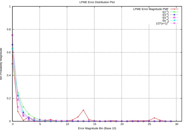
3.5.4 Error distribution and Encoding Selection . . . 36
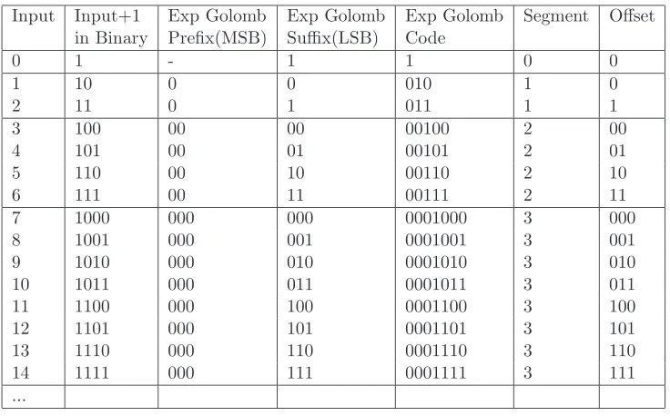
3.5.5 LPME+EXPG+ZLIB encoding scheme . . . 40
3.5.6 Improving Longest Prefix Matching performance using Gray Codes . 42 3.6 Residual Lossless Schemes (SBB-R-CR-Lossless) based on Block Based Mo-tion EstimaMo-tion and Histogram Packing . . . 45
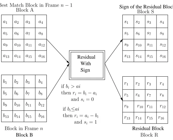
3.6.1 Residual With Sign . . . 46
3.6.2 Residual Without Sign . . . 48
3.7 Residual Lossy Schemes (SBB-R-CR-Lossy) with an Intra/Key Frame . . . 51
4 Results 53 4.1 Bitrate Comparison . . . 53
4.1.1 Discussion of the Bitrate Results . . . 55
4.2 Time Evaluation . . . 71
4.2.1 Discussion of the Time Results . . . 71
4.3 Comparison of SBB-R-LPME-ZLIB And SBB-R-GRAY-LPME-ZLIB . . . . 86
4.4 Bitrate Vs Encoding Time . . . 89
5 Future Work 104 6 Conclusion 107 Bibliography 109 7 Appendix 113 7.1 Zlib . . . 113
7.2 Lagarith . . . 114
7.3 JPEG-LS . . . 114
7.4 Binary Code to Gray Code Conversion . . . 115
7.5 Gray Code to Binary Code Conversion . . . 118
7.6 Searching for the right parameters for JASPER-JPEG-2000 encoding . . . . 120
7.6.1 Definitions . . . 120
7.6.2 Parameters . . . 122
7.6.3 Bitrates . . . 127
7.6.4 Profiling Analysis . . . 129
List of Figures
1.1 Typical Design Requirements of Video Communication Systems . . . 1
1.2 Classification of Video Encoding Schemes based on Replenishment type . . 12
2.1 (SBB-NR-CR) Non-Residual Conditional Replenishment Based Video En-coding System Block Diagram . . . 13
2.2 Simple Block Based-Non-Residual Conditional Replenishment (SBB-NR-CR) Encoding Process . . . 14
2.3 Effect of lossy encoding on video after SBB-NR-CR . . . 17
2.4 (a)Ringing Effect for Lossy encoding (b) Lossless encoding . . . 18
2.5 Effect of ringing effect in the previous ”Video” image on the current ”Video” image . . . 19
2.6 Bitrate@30fps comparison of schemes using JPEG-2k, with and without SBB-NR-CR . . . 20
2.7 Comparison of JPEG-LS and JPEG-2000 . . . 23
3.1 Clean Image Lossless Encoding . . . 27
3.2 SBB-NR-CR-Histogram Packing Based Video Encoding Scheme . . . 32
3.3 Longest Prefix Motion Estimation Working . . . 37
3.4 LPME Error Distribution . . . 38
3.5 Huffman Tree for some Geometrically Distributed Symbols . . . 39
3.6 Golomb Codes . . . 39
3.7 Exp-Golomb Codes . . . 40
3.8 LPME+EXPG+ZLIB Conditional Replenishment System Block Diagram . 41 3.9 GRAY+LPME+EXPG+ZLIB Conditional Replenishment System Block Di-agram . . . 43
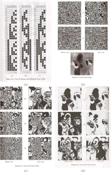
3.10 (a) Binary, Gray Comparison (b) bit-planes 1, 2 (c) bit-planes 3, 4, 5 (d) bit-planes 6, 7, 8 . . . 44
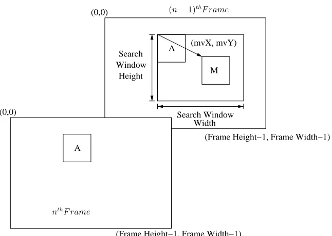
3.11 Motion Estimation Brute Force Technique . . . 45
3.12 Residual With Sign . . . 46
3.13 SBB-R-CR-SAD Based Motion Estimation With Sign, Block Diagram . . . 47
3.14 SBB-R-CR-SAD Based Motion Estimation With Sign, Histogram Packed, Block Diagram . . . 48
3.16 SBB-R-CR-SAD Based Motion Estimation Without Sign, Block Diagram . 50 3.17 SBB-R-CR-SAD Based Motion Estimation Without Sign, Histogram Packed,
Block Diagram . . . 51
4.1 Gamma Compression Curve used for Creating Sparse Histograms . . . 54
4.2 Bitrate@30 fps For Forest Sequence with 4x4 SBB-CR . . . 57
4.3 Bitrate@30 fps For Forest Sequence with 8x8 SBB-CR . . . 58
4.4 Bitrate@30 fps For LGE Sequence with 4x4 SBB-CR . . . 59
4.5 Bitrate@30 fps For LGE Sequence with 8x8 SBB-CR . . . 60
4.6 Bitrate@30 fps For Highway Sequence with 4x4 SBB-CR . . . 61
4.7 Bitrate@30 fps For Highway Sequence with 8x8 SBB-CR . . . 62
4.8 Bitrate@30 fps For Highway Sparse Sequence with 4x4 SBB-CR . . . 63
4.9 Bitrate@30 fps For Highway Sparse Sequence with 8x8 SBB-CR . . . 64
4.10 Bitrate@30 fps For NoVideo Sequence with 4x4 SBB-CR . . . 65
4.11 Bitrate@30 fps For NoVideo Sequence with 8x8 SBB-CR . . . 66
4.12 Bitrate@30 fps For QuarterScreenForeman Sequence with 4x4 SBB-CR . . 67
4.13 Bitrate@30 fps For QuarterScreenForeman Sequence with 8x8 SBB-CR . . 68
4.14 Bitrate@30 fps For DuckTales Sequence with 4x4 SBB-CR . . . 69
4.15 Bitrate@30 fps For DuckTales Sequence with 8x8 SBB-CR . . . 70
4.16 Encoding Time For Forest Sequence with 4x4 SBB-CR . . . 72
4.17 Encoding Time For Forest Sequence with 8x8 SBB-CR . . . 73
4.18 Encoding Time For LGE Sequence with 4x4 SBB-CR . . . 74
4.19 Encoding Time For LGE Sequence with 8x8 SBB-CR . . . 75
4.20 Encoding Time For Highway Sequence with 4x4 SBB-CR . . . 76
4.21 Encoding Time For Highway Sequence with 8x8 SBB-CR . . . 77
4.22 Encoding Time For Highway Sparse Sequence with 4x4 SBB-CR . . . 78
4.23 Encoding Time For Highway Sparse Sequence with 8x8 SBB-CR . . . 79
4.24 Encoding Time For NoVideo Sequence with 4x4 SBB-CR . . . 80
4.25 Encoding Time For NoVideo Sequence with 8x8 SBB-CR . . . 81
4.26 Encoding Time For QuarterScreenForeman Sequence with 4x4 SBB-CR . . 82
4.27 Encoding Time For QuarterScreenForeman Sequence with 8x8 SBB-CR . . 83
4.28 Encoding Time For DuckTales Sequence with 4x4 SBB-CR . . . 84
4.29 Encoding Time For DuckTales Sequence with 8x8 SBB-CR . . . 85
4.30 Encoding Time Plots for LPME and GRAY-LPME . . . 87
4.31 Bitrate Plot for LPME and GRAY-LPME . . . 88
4.32 Bitrate@30 fps Vs Encoding Time For Forest Sequence with 4x4 SBB-CR . 90 4.33 Bitrate@30 fps Vs Encoding Time For Forest Sequence with 8x8 SBB-CR . 91 4.34 Bitrate@30 fps Vs Encoding Time For LGE Sequence with 4x4 SBB-CR . . 92
4.35 Bitrate@30 fps Vs Encoding Time For LGE Sequence with 8x8 SBB-CR . . 93
4.36 Bitrate@30 fps Vs Encoding Time For Highway Sequence with 4x4 SBB-CR 94 4.37 Bitrate@30 fps Vs Encoding Time For Highway Sequence with 8x8 SBB-CR 95 4.38 Bitrate@30 fps Vs Encoding Time For Highway Sparse Sequence with 4x4 SBB-CR . . . 96
4.40 Bitrate@30 fps Vs Encoding Time For NoVideo Sequence with 4x4 SBB-CR 98
4.41 Bitrate@30 fps Vs Encoding Time For NoVideo Sequence with 8x8 SBB-CR 99
4.42 Bitrate@30 fps Vs Encoding Time For QuarterScreenForeman Sequence with
4x4 SBB-CR . . . 100
4.43 Bitrate@30 fps Vs Encoding Time For QuarterScreenForeman Sequence with 8x8 SBB-CR . . . 101
4.44 Bitrate@30 fps Vs Encoding Time For DuckTales Sequence with 4x4 SBB-CR 102 4.45 Bitrate@30 fps Vs Encoding Time For DuckTales Sequence with 8x8 SBB-CR 103 5.1 Parallelized, Pipelined SBB-NR-CR . . . 106
7.1 Binary Gray KMAP . . . 117
7.2 Binary to Gray Conversion Logic Diagram . . . 117
7.3 Gray Binary KMAP . . . 119
7.4 Gray To Binary Conversion Logic Diagram . . . 119
7.5 (a) Reversible(Lossless) DWT, Resolution Levels and PSNR Vs BPP graph (b) Irreversible(Lossy) DWT , Resolution Levels and PSNR Vs BPP graph (c) Tile size plots with no MCT(fixed Level) (d) Tile plots with ICT (fixed Level) . . . 124
7.6 Encoding Time( sec) for the Different Code Block Sizes . . . 126
List of Tables
2.1 Comparison of Quarterscreen Video SBB-NR-CR encoding schemes . . . 16
2.2 Rate comparison of schemes using JPEG-2k, with and without CR . . . 21
2.3 PSNR and Bitrate of the Lossy-Video Scheme . . . 21
2.4 JPEG-2000 Vs JPEG-LS Bitrates . . . 22
2.5 JPEG-2000 Vs JPEG-LS Encoding Timings . . . 23
3.1 Exponential Golomb Codes . . . 40
7.1 Truth table for 4 bit Gray code to 4 bit Binary Code . . . 116
7.2 Truth table for 4 bit Gray code to 4 bit Binary Code . . . 118
Chapter 1
Introduction
1.1
Overview of Video Communication Systems
Figure 1.1: Typical Design Requirements of Video Communication Systems
Figure 1.1 shows the different requirements from a typical video communication
system. These constraints are typically contradictory [1], in the sense that trying to optimize
for one is generally unoptimal for the others, with the notable exception of attempting to
achieve low complexity and high quality at the same time. It is believed that finding a
specific solution to a distributive or interactive video communications problem has to be
robustness against channel errors, and the associated implementation complexity. Analyzing
these tradeoffs and proposing solutions to various video communication problems, is the field
of video communications [1].
1.2
Project Goals
The project was motivated by a desire to seek a high quality, computationally
lightweight, and low bitrate video encoding scheme, and in the process evaluate the
perfor-mance of the proposed schemes.
1.3
Literature Survey and Scientific Contribution of this work
Lossy video coding is now a maturing subject, albeit still not an exact science.
It is largely predicated on the structure of image coding, which is a more mature
sub-ject. While no global optimization approach yet exists for the problem of image coding, in
practice image coding has now stabilized into a 3-stage process of transform, quantization,
and entropy coding. Video coding goes a step further, and incorporates a motion
estima-tion/compensation loop, giving it both temporal and spatial decorrelation. This technique
of exploiting both the temporal and spatial correlation in a group of frames is known as
Conditional Replenishment, which can be done either as a residual-error based scheme or
as replenishment of entire blocks that have changed across images, which we call as
Non-Residual based scheme. While the follow-on stages of quantization and entropy coding have
seen improvements in recent standard designs, it is primarily the subject of advanced spatial
and temporal decorrelation that has been the focus of recent designs, especially the latest
international standard: ITU/H.264 — ISO/IEC/MPEG-4 Pt. 10 (AVC) [4]. While
atten-tion is being given to seek optimality vis-a-vis bitrate-distoratten-tion, relatively less attenatten-tion
has been given to the time complexity of these schemes. The reason lossy coding has gained
popularity is because it is possible to achieve great deal of compression at a relatively small
cost of quality, and thus is the de-facto way to do video compression for applications such
as televisions etc.
On the other hand, although lossy video coding has been studied extensively in
in the literature because of its very high bandwidth demands rendering it impractical for
everyday use. Lossless video encoding has applications in medical and scientific applications,
studio quality archival purposes [5], and extremely high quality video playback.
However, although the field of lossless video encoding has not been extensively
dealt with in scientific literature, there is a cottage industry around the development of
proprietary lossless video codecs. Several companies and individual people have developed
their own codecs. To name a few they are: Alparysoft lossless codec, MSU, CorePNG,
YULS, FFV1, Flash Screen Video, HuffYUV, Lagarith, MSU lossless Codec, Pegasus
Loss-less JPEG, Sheer Video, VMWare Video, CamStudio Screen Codec, DosBox Capture Codec,
Fraps, Microsoft Screen Codec, TechSmith Screen Capture Codec, Flash Video Encoder etc.
A study undertaken by the MSU Graphics and Media Lab (Video Group), in
March 2007 [7], compares several of these existing lossless video encoders, and leads to
the conclusion that amongst the codecs that they evaluated, in Video Capture and Video
Editing area, the overall clear winner is Lagarith [29]. In Maximum Compression area the
overall winner is YULS and the most balanced and flexible codec is FFV1 (relatively good
speed and high compression for various presets). Their study shows that typically, the
compression ratio achieved by the best lossless codec is around 3.15 [7], which can be more
than the compression ratio achieved by H.264 (Best Quality). We also compare some of these
codecs including the MSU codec with our codec, and confirm their findings. Through our
results we see that our codec performs better than Lagarith for some of the sequences, but
we note that MSU consistently gives better bitrates than the codec presented in this work.
However, MSU takes much more time to do the encoding than the codec presented herein.
We thus claim that the codec presented in this work is amongst the best
low-computation-time and low-bitrate lossless codecs around as of today. MSU is a proprietary codec and the
algorithm has not been released. Lagarith is quite fast as we also confirm, but not always
better than the work presented herein. In terms of achieving a good competitive balance
of compression rate and encoding speed, this work does present a fast lossless Conditional
Replenishment based lossless codec.
In the design of video encoding schemes, considerable effort has also gone into
the design of high quality but low delay, real time transmission of desktop images, leading
to the development of remote desktop applications. These applications typically employ a
computing (SBC) model is fast becoming an increasingly popular approach for delivering
computational services with reduced administrative costs and better resource utilization.
Nieh et. al. in [8], examine how effectively SBC architectures support multimedia
applica-tions. Typically, the approach used for remote desktop applications, is to encode only the
blocks that have changed across consecutive images, and then transfer this encoded data
over the channel. As noted before, this approach is called as Conditional Replenishment.
In this thesis we first classify video encoding schemes in their ability to do Residual
Con-ditional Replenishment and Non-Residual ConCon-ditional Replenishment, and evaluate the
performance of each. Several proprietary codecs developed, fall into the categories that
would be evaluated in the thesis.
Amongst existing Server-based video encoding applications, Virtual Network
Com-puting (VNC) is a popular application for encoding of desktop screens and transferring them
over the network, typically for remote desktop use. The VNC standard proposes the use
of the following approaches to encode data and is known as the RemoteFrameBuffer(RFB)
Protocol.
1. Raw : The raw encoding simply sends width*height pixel values. All clients are
required to support this encoding type. Raw encoding minimizes processing time.
2. CopyRect: The Copy Rectangle encoding principle is to copy updates from other
areas of the screen if they already exist there. The only data sent is the location of a
rectangle from which data should be copied to the current location. Copyrect could
also be used to efficiently transmit a repeated pattern. The VNC Project however
does not have a scheme to decide efficiently which areas of the screen are the most
likely candidates for thie copyrect.
3. RRE: The Rise-and-Run-length-Encoding is basically a 2D version of run-length
en-coding (RLE). In this enen-coding, a sequence of identical pixels are compressed to a
single value and repeat count. In VNC, this is implemented with a background color,
and then specifications of an arbitrary number of subrectangles and color for each.
This is an efficient encoding for large blocks of constant color.
4. CoRRE: This is a minor variation on RRE, using a maximum of 255x255 pixel
general more efficient, because the savings from sending 1-byte values generally
out-weighs the losses from the (relatively rare) cases where very large regions are painted
the same color.
5. Hextile: Here, rectangles are split up in to 16x16 tiles, which are sent in a
predeter-mined order. The data within the tiles is sent either raw or as a variant on RRE.
Hextile encoding is usually the best choice for using in high-speed network
environ-ments (e.g. Ethernet local-area networks).
6. Zlib: Zlib uses zlib data compression library to compress raw pixel data. This encoding
achieves good compression. Support for this encoding is provided for compatibility
with VNC servers that might not understand Tight encoding which is more efficient
than Zlib in nearly all real-life situations.
7. Tight: Like Zlib encoding, Tight encoding uses zlib library to compress the pixel
data, but it pre-processes data to maximize compression ratios, and to minimize CPU
usage on compression. Also, JPEG compression may be used to encode color-rich
screen areas. Tight encoding is usually the best choice for low-bandwidth network
environments (e.g. slow modem connections).
In [8], Nieh et. al. report that typically, using Server Based Computing, a
com-pression gain of 2 or more is generally achieved at an acceptable quality. In our findings
in this thesis, we will also see that we achieve similar compression performance using
Non-Residual, block based Conditional Replenishment using Zlib. We would also demonstrate
the performance of a scheme quite similar in spirit to VNC Tight encoding. The VMWare
Video Codec, uses this VNC RemoteFramebuffer protocol [9]. The codec SBB-NR-CR-ZLIB
presented in this thesis is very similar to VMware Video Codec and VNC-Zlib encoding.
Further, a high quality image compression system, has been described by Nakao
et. al. in [2] wherein they use JPEG-2000 to encode the blocks that have changed across
consecutive images. The codec SBB-NR-CR-JPEG-2000 presented in the second chapter of
this thesis, is comparable with the codec presented by Nakao. et. al [2]
In [5], Memon and Sayood investigate lossless video coding techniques by extending
the 2-D prediction based methods used in lossless image coding into 3-D, thus considering
block based difference technique for motion compensation that has been so successfully
used in lossy encoding does not work well when used with lossless compression since the
statistical properties of the residuals are different from still images. A similar 3-D approach
has been proposed by Brunello et. al. [10], and another similar but embedded approach
has been proposed by [13]. Our work confirms the findings leading to a similar conclusion
that residual encoding might not be always useful. Implementing an improved variant of
the motion estimation error metric, based on minimizing the prediction error of the lossless
image encoding scheme, instead of using SAD, as proposed by Memon et. al. [5] is part of
future work. Also, the optimal prediction idea proposed by [10] is part of the future work,
although in this thesis we do work on a 3-D prediction, but our work cannot be considered
optimal. Also, the optimal prediction considered in [10] leads to around 10% improvement
in bitrate, which thus if applied to the codecs based on Motion Estimation that we present,
would still lead to a bitrates obtained less than those obtained by the most efficient codec
considered in this work.
In [12], Alzina et. al. discuss a novel method based on a fixed database model using
longest prefix matching with the elements in the database(dictionary), followed by enhanced
run length coding, followed by lossless encoding, and they propose lossy extensions to it.
Through this work, we also attempt a similar longest prefix matching motion estimation,
however, our results do not compare favorably against theirs. Discussion about why such a
result was obtained would be considered in the thesis.
To the best of the author’s knowledge, no equivalent study of the schemes presented
herein and a classification of video encoding schemes as given herein has been reported in
the literature to date. Thus, through this work, we make contribution to the literature
for lossless encoding of video by describing the design and performance gains/losses that
can be achieved through use some block based Conditional Replenishment schemes. We
independently confirm the findings of [5], [12], and propose directions of future research.
We also confirm the findings of [3] of the gains achieved by Histogram Packing, and propose a
schematically simple and lightweight video encoding scheme that outperforms several other
propreitary schemes. We also make the contribution of classifying existing video encoding
1.4
Approach and Organization of the thesis
The thesis starts with a model of Conditional Replenishment where in, there is no
motion estimation (and correspondingly no motion compensation) and Conditional
Replen-ishment is instead done with a very simple boolean-block-based-pel differentiator, which
checks, per block, if any pixel/pel in the block is different from the corresponding pixel/pel
in the block of the previous image.
If even one pel differs in the entire block, across any one of the components, then
that entire block of pixels is tagged that it needs to be Conditionally Replenished. That
block is marked present in the ”text image”, and the pixel-data in the block is put into the
corresponding location in the ”video image”.
This process is repeated for every block in the current image. At the end of
this process we get a ”text image” signifying a map of presence of blocks that have been
Conditionally Replenished, and the ”video image” which contains the data necessary for
reconstructing the image at the decoder. We call this process as Simple Block Based,
Non-Residual, Conditional Replenishment (SBB-NR-CR). Now, once this scheme for doing
Conditional Replenishment has been established, we will experiment with its components.
Applying this technique to the images that make up a video sequence, make these schemes
video encoding schemes.
Figure 1.2 shows the schemes that are presented in this work. In this figure, the
schemes marked with ”FW” mean future work, and the schemes that are numbered are
discussed in this work. The organization of the thesis is as follows:
1. The first section of the thesis would start off with describing how Simple Block Based,
Non-Residual, Conditional Replenishment (SBB-NR-CR), followed by lossy/lossless
image coding leads to a compression gain. This chapter will then put forth an
argu-ment for the lossless encoding of the ”Text image” created after SBB-NR-CR. Then the
chapter would discuss how SBB-NR-CR followed by lossy JPEG-2000 of the ”Video
Image” leads to results worse than the ones achieved with SBB-NR-CR followed by
lossless JPEG-2000 encoding of the ”Video Image”. By being convinced of this fact,
an alternative to JPEG-2000, that being JPEG-LS, would be considered as a probable
candidate for fast lossless image coding. It would be confirmed by experiments that
compression scheme of our choice for doing SBB-NR-CR followed by lossless encoding
of the ”Video Image”. This scheme would be called as SBB-NR-CR-JPEG-LS.
2. In this second section, we would work on an attempt to improve the compression
gains achieved in SBB-NR-CR-JPEG-LS. Most of the results of this work are in the
negative in the sense of not leading to any compression improvement, except for the
improvement achieved by online Histogram Packing for sparse histogram images, and
the compression gain achieved for some images using ZLIB instead of JPEG-LS. The
chapter considers the motivation for trying out the following approaches and explains
the theory behind them.
(a) CleanImage Lossless Encoding Schemes
i. CleanImage JPEG-LS: This is also called Motion JPEG-LS.
ii. CleanImage ZLIB: This is also called Motion ZLIB.
(b) SBB-NR-CR-Lossless using ZLIB: In this scheme, the ”text” and ”video” image
is encoded using ZLIB. This scheme is similar to Tight-VNC-ZLIB.
(c) Non-Residual Lossless Schemes (SBB-NR-CR-Lossless) based on Histogram
Pack-ing
i. NR-CR-OfflineHistogramPacked-JPEG-LS: Image obtained after
SBB-NR-CR subjected to offline Histogram Packing followed by JPEG-LS
encod-ing.
ii. CR-OnHistogramPacked-JPEG-LS: Image obtained after
SBB-NR-CR subjected to Online Histogram Packing, followed by JPEG-LS encoding.
iii. SBB-NR-CR-ZLIB: Encoding of both, Video image and Text Image using
ZLIB.
iv. CR-OfflineHistogramPacked-ZLIB: Image obtained after
SBB-NR-CR subjected to offline Histogram Packing, followed by ZLIB encoding.
v. SBB-NR-CR-OnHistogramPacked-ZLIB: Image obtained after SBB-NR-CR
subjected to Online Histogram Packing, followed by ZLIB encoding.
(d) Non-Residual Lossy Schemes (SBB-NR-CR-Lossy) with Intra Frame/Key Frame
(e) Residual Lossless Schemes (SBB-R-CR-Lossless) based on Longest Prefix
Match-ing Motion Estimation and Gray Code Variant
i. SBB-R-CR-LPME-ZLIB: Longest Prefix Matching Motion Estimation (LPME)
using XOR (addition modulo 2), followed by ZLIB encoding of the bitstream.
ii. SBB-R-CR-Gray-LPME-ZLIB: LPME using Gray Codes.
(f) Residual Lossless Schemes (SBB-R-CR-Lossless) based on SAD Motion
Estima-tion and Histogram Packing
i. SBB-R-CR-SAD-WithSign-JPEG-LS: Simple Block Based, Residual
Condi-tional Replenishment. The Residual is found out using Motion Estimation
with sign, followed by JPEG-LS.
ii. SBB-R-CR-SAD-WithoutSign-JPEG-LS: Simple Block Based, Residual
Con-ditional Replenishment. The Residual is found out using Motion Estimation
without sign, followed by JPEG-LS.
iii. SBB-R-CR-SAD-WithSign-ZLIB: Simple Block Based, Residual Conditional
Replenishment. The Residual is found out using Motion Estimation with
sign, followed by ZLIB.
iv. SBB-R-CR-SAD-WithoutSign-ZLIB: Simple Block Based, Residual
Condi-tional Replenishment. The Residual is found out using Motion Estimation
without sign, followed by ZLIB.
v. SBB-R-CR-SAD-WithSign-OnlineHistogramPacked-JPEG-LS:
SBB-R-SAD-WithSign undergoing Online Histogram Packing, followed by JPEG-LS.
vi. SBB-R-CR-SAD-WithoutSign-OnlineHistogramPacked-JPEG-LS:
SBB-R-SAD-WithSign undergoing Online Histogram Packing, followed by JPEG-LS.
vii. SBB-R-CR-SAD-WithSign-OnlineHistogramPacked-ZLIB: SBB-R-SAD-WithSign
undergoing Online Histogram Packing, followed by ZLIB.
viii. SBB-R-CR-SAD-WithoutSign-OnlineHistogramPacked-ZLIB:
SBB-R-SAD-WithSign undergoing Online Histogram Packing, followed by ZLIB.
(g) Residual Lossy Schemes (SBB-R-CR-Lossy) with an Intra/Key Frame:
This thesis does not cover these schemes and comparison with the codecs
pre-sented herein is part of future work. This is the category into which the MPEG-2,
3. This section will give the Benchmarking Results i.e. performance comparison of each
of the schemes outlined here with reference to bitrate and encoding times, comparing
them with codecs such as H.264 High Profile, Fidelity Range Extensions, with QP=1,
i.e. highest quality that can be achieved using H.264, with AlparySoft’s Lossless codec,
with MSU, with Lagarith, with Techsmith Screen Capture codec which is used by the
Camtasia desktop grabbing tool and the Lossless Adobe Flash Codec.
4. The fourth section would be the conclusions section, which would discuss that lossless
SBB-CR is a good way to do SBB-NR-CR especially if high quality but low playback
delay and real time encoding is desired. Further, at relatively similar computational
cost, a lossy SBB-NR-CR leads to a poorer quality video, and lossy SBB-NR-CR
does not lead to significantly less bitrate because of additional content in the video
image (because of the error in the reconstructed image). This work further shows
that SBB-NR-CR-HistPacked-JPEG-LS gives the best performance amongst all the
schemes tested and for all the sequences tested when the sequence is made up of natural
images. The work further shows that SBB-NR-CR-ZLIB can give good performance in
comparison with Lossless Flash Video Encoder for sequences with no natural images,
and containing high frequency components. This work shows that the promise of
LPME-ZLIB and SAD based lossless video encoding cannot be achieved using the
techniques as has been used here and that it needs some more careful design. The
work also shows that SBB-NR-CR-OnlineHistPacked-JPEG-LS is a method that is
competitive to the best lossless video codecs known.
5. The fifth section would describe directions of future work, and scope for parallelization.
1.5
Definitions
This section describes the definitions of various terms used in the thesis.
1. Compression Rate = Image Size Af ter CompressionImage Size bef ore compression ((in unit Uin unit U))
2. Bits per Pixel (bpp)β = compression Rate * δ bits/pixel, δ = 24 bits/pixel, for our
3. Bitrate@α frames per second (fps) = (Image Height in pixels * Image Width in pixels
* β * α fps) bits per second(bps).
4. SBB-NR-CR : Simple Block Based, Non-Residual, Conditional Replenishment
5. SBB-R-CR : Is an abbreviation for SBB-NR-CR-R, meaning Simple Block Based,
Residual, Conditional Replenishment.
6. PSNR : The phrase peak signal-to-noise ratio, often abbreviated PSNR, is an
engi-neering term for the ratio between the maximum possible power of a signal and the
power of corrupting noise that affects the fidelity of its representation. Because many
signals have a very wide dynamic range, PSNR is usually expressed in terms of the
logarithmic decibel scale (db). The power of a signal x(t) is usually represented by
x2(t) in the spirit of electrical power which states that the amount of work that is
done by an electric current is P = I2R, or P = V2/R. Thus if the signal x(t) is a
measure of the current or the voltage at time t, then its power is approximated to be
x2(t). If we consider two imagesgandg′, whereg′ is a noisy approximation ofg, then
the Mean Squared Error (MSE) is given as :
M SE = mn1 Pm−1
i=0 Pn−1
i=0||g(i, j)−g′(i, j)|| 2
P SN R = 10.log10(
M AX2
g
M SE ) = 20.log10(
M AXg
M SE )
where M AXg is the highest intensity value in the intensity range of g depending on
the bit depth. For color images with three RGB values per pixel, the definition of
PSNR is the same except the MSE is the sum over all squared value differences divided
Chapter 2
Simple Block Based, Non-Residual,
Conditional Replenishment
2.1
Simple Block Based, Non-Residual, Conditional
Replen-ishment (SBB-NR-CR) Based Video Encoding System,
Architecture Design
CR
Lossless/lossy encoding
Module
Lossless/lossy encoding
Module Decoding
Module
Decoding Module
Previous Image Decoded
(RGB) Current
Image Previous
Image (RGB)
Image
Image Video Text
Output Image Decoder Side
Encoder Side
Data flow during the operation of the transition from the nth and the (n+1)th image (n>1) Data flow during operation on the nth image (n>1)
Stage Y Stage X
Bitstream Rx Tx
Tx Rx
Bitstream SBB−NR
Comparator A B C D A B C D A B C D A B C D 1 1 1 Frame n, text block
Per Pel Frame (n−1) Reconstructed block E F G H Frame n
Clean Block Clean Block
Frame n
Frame n, video block after SBB−NR−CR
after SBB−NR−CR Frame n, text block
0 0 0 0 0 0 0 0
across consecutive Frames across consecutive Frames
Reconstructed block Frame (n−1)
(X, Y) (X, Y)
(X, Y) (X, Y)
(X, Y)
(X, Y) (X, Y)
(X, Y)
SBB−NR−CR with different block values SBB−NR−CR with same block values
(A) (B)
Per Pel Comparator
Frame n, video block after SBB−NR−CR
after SBB−NR−CR 1
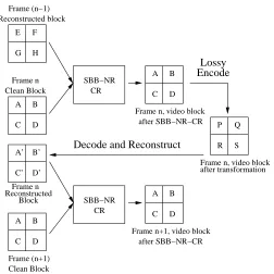
Figure 2.2: Simple Block Based-Non-Residual Conditional Replenishment (SBB-NR-CR) Encoding Process
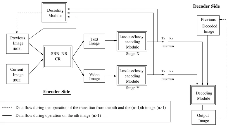
Figure 2.1 shows the Conditional Replenishment encoding/decoding scheme block
diagram. For all frames(n) withn >1, we use the encoding scheme as shown in Figure 2.1,
and the first frame is transferred over the channel as it is without any compression. The
Simple Block Based, Non-Residual, Conditional Replenishment (SBB-NR-CR) module as
shown in the Figure 2.1 operates using the technique shown in Figure 2.2. The principle
behind the operation of SBB-NR-CR is as follows: Consider a block in the framenlocated
at position (X, Y). Lets assume without loss of generality, that this block is made up of
pels A, B, C and D. Now, consider the block in the previous reconstructed frame i.e. in
reconstructed (n−1)thframe located at the same position (X, Y). Then, each pel from the
block ”ABCD” is compared with the block ”EFGH” from the previous frame. Even if 1 pel
differs in value, then the entire block ”ABCD” is carried forward, as it is, to the ”video”
image, and the ”text” image is marked with 1s as shown in Figure 2.2 (a). Figure 2.2 (b)
shows what is to happen when the block in the previous frame i.e. (n−1)th reconstructed
frame is exactly same as the block in the nth frame at position (X, Y). In this case, the
text image is marked with 0s and the video image is also marked with 0. This process is
called Simple Block Based Non-Residual Conditional Replenishment, and this represents
the SBB-NR-CR block shown in Figure 2.1.
The SBB-NR-CR process takes two images as input, the current image and the
step is encoding these two images. Stage X and Stage Y as shown in Figure 2.1 are used
to accomplish this goal. We can do lossy as well as lossless encoding of these images.
The dotted line in the figure is used to show that the previous image during the
encod-ing of the (n+ 1)th image is to be constructed from the existing (n−1)th frame and the
decoded/reconstructed differential/residual data, because doing so guarantees that the
re-constructed images on the decoder side has the same quality (PSNR) as could have been
observed after the decoding of an image on the encoder side.
2.2
Encoding of ”Text” image and ”Video” image
We will discuss the following approaches for encoding the ”text” and ”video” image
data
1. Lossy text scheme: This leads to a very minor reduction in bitrate over lossless text.
2. Lossless text and lossy video scheme: Results show that for the image sets considered,
lossy video leads to an overall bitrate higher than the one achieved by lossless
SBB-NR-CR, despite the ability of SBB-NR-CR lossy encoding to encode at arbitrary
bitrates.
3. Lossless test and lossless video, which is the scheme that gave the best results for
SBB-NR-CR.
We would use the wavelet based JPEG-20001 as the image encoding engine to compress the
text image and the video image. An analysis of JPEG-2000 parameters was made and the
encoding was parameterized on the parameters that showed the best performance.2
2.2.1 Lossy Text
In this scheme, we use JPEG-2000 in the lossy mode to compress the ”text” image
obtained after SBB-NR-CR. Because the text acts like a map for the ”video” image data,
having a lossy ”text” leads to misconstruction of the ”video” reconstructed image. It is
seen that because the ”text” image is made up of only 0s and 1s, and is more amenable
to run length coding than the video image, it is compressed to very small files, even when
1
See Appendix
2
using the lossless entropy coding in the JPEG-2000. Doing a lossy compression for this text
portion, leads only to a degradation of quality at tiny bitrate savings. Consequently the
idea of doing a lossy text encoding was dropped.
2.2.2 Lossless Text, Lossy Video
The motivation for checking the performance of lossless text and lossy video was
that lossy encoding allows us to compress a single image at an arbitrary rate. These numbers
were collected by running SBB-NR-CR-JPEG-2000 Quarterscreen Forest sequence and LG
sequence and then finding the mean over all these sequences. On average, for quarter
screen video sequences, it can be seen from Table 2.1 that lossy SBB-NR-CR performs
worse than lossless SBB-NR-CR for our sample image set. Note that here, the input set
is only Quarterscreen, and we would need to take more measurements before we can say
whether lossless video is better/worse than lossy video. In this section, we will talk about
why we have observed such a result. The next section about lossless video, will put forth
an argument to decide the winner amongst lossless video and lossy video.
Table 2.1: Comparison of Quarterscreen Video SBB-NR-CR encoding schemes
Scheme Overall Compression Rate Bits Per Pixel PSNR Bitrate@30fps(bps)
Text 0.2 4.99 48.45 138,018,816
Lossless, 48.65
[email protected] 48.65
Text,Video 0.06 1.44 INF 39,813,120
Lossless INF
INF
No CR; 0.06 1.44 31.40 39,813,120
[email protected] 31.53
31.53
Reason for poorer performance of lossy NR-CR compared to lossless
SBB-NR-CR
This effect can be explained by looking at Figure 2.3. This figure shows how lossy
encoding of the previous video image, can lead to video image blocks that would be absent
had we done lossless encoding for the previous video image. As has been shown in Figure
2.3, if the reconstructed block in the n−1th frame is with pel values ”EFGH”, and the
Frame n, video block
A B
C D
A B
C D
A B
C D
A B
C D
P Q
R S
A’ B’
C’ D’
SBB−NR CR SBB−NR
CR
E F
G H
Block Reconstructed Reconstructed block
Frame n Frame (n−1)
Frame (n+1) Clean Block Clean Block
Frame n
Frame n+1, video block after SBB−NR−CR Frame n, video block after SBB−NR−CR
Lossy Encode
Decode and Reconstruct
after transformation
Figure 2.3: Effect of lossy encoding on video after SBB-NR-CR
SBB-NR-CR, the output would be the block ”ABCD” assuming that the block ABCD, and
EFGH differ in at least 1 pel value. We need to make this assumption because we are trying
to demonstrate why SBB-NR-CR lossless performs better than SBB-NR-CR lossy. If we
do not make this assumption, then after SBB-NR-CR we would know that this block has
not changed across consecutive frames, and we not bother encoding it. Hence, we assume
that block ABCD, and block EFGH differ in at least 1 pel value. If we attempt to encode
this video image after SBB-NR-CR using lossy encoding, like JPEG-2000 in lossy mode,
then, after transformation by JPEG-2000, the block would appear to be say ”PQRS”. After
decoding this PQRS block using JPEG-2000, we are going to see some loss because this
block was encoded lossily. Consequently therefore, if we now reconstruct the block, we
would get the block A’B’C’D’ which could be different than the block ”ABCD”. Here we
consider the case in which it IS different, which is a reasonable assumption. Further now, if
the next frame, i.e. (n+ 1)th frame contains that same block, in the same coordinates, then
after SBB-NR-CR, the block ”ABCD” would be encoded again. Note that had we encoded
the previous video image losslessly, then after reconstruction, we would have got back the
(a) (b)
Figure 2.4: (a)Ringing Effect for Lossy encoding (b) Lossless encoding
for the (n+ 1)th frame.
Figure 2.4 shows two images, in which one was encoded losslessly using
JPEG-2000, and the other was encoded lossily. It can be seen that the Figure 2.4 (a) has much
perceptual (and PSNR as well) poorer quality than 2.4 (b). It can be noted that at sharp
edges there is a smearing effect occurring. This effect is the ringing effect which comes as
an artifact introduced by DWT subject to lossy quantization. Note that DWT reversible,
if not subjected to a quantization loss, when reconstructed/decoded leads to a perfect
reconstruction and leads to no ringing effects. This is because of using reversible mother
wavelets for the reversible JPEG-2000. In the SBB-NR-CR encoding of the next frame, this
newly reconstructed image would be used as the reference as explained before. An example
of how a lossy encoding of the previous video image led to distortion in the reconstructed
previous image, thereby causing stray blocks in the current video image is shown in Figure
2.5.
As a consequence of this ringing effect, the video part image size keeps increasing.
The video blocks can reduce only under the condition if a new block undergoes no
quanti-zation loss in the lossy encoding process. In such cases, the block is made of low frequency
components, and is not affected by the quantization. However, whenever the block contains
high frequency components, which is not so atypical for unnatural sequences such as
desk-top grabs, then that leads to error propagation, and leads to loss in compression efficiency.
With reference to Figure 1.2, we are discussing about Scheme 8, and comparing it with
Scheme 3. This error propagation explains the results seen in Table 2.1, that the lossless
Figure 2.5: Effect of ringing effect in the previous ”Video” image on the current ”Video” image
In order to convince ourselves whether a SBB-NR-CR-Lossy is really worse than
Lossless, we would need to first measure the performance of
SBB-NR-CR-Lossless. This is done in the next section.
2.2.3 Lossless Text, Lossless Video
This section is divided into two sub-parts. In the first part we measure the
per-formance of SBB-NR-CR with lossless text and lossless video in comparison with
Clean-Image compression using JPEG-2000, which is called as MJPEG when enclosed in an AVI
header. Once we are through with this test we would have an average compression rate that
was achieved by the CR-Lossless. In order to see the performance of
SBB-NR-CR-LossyWithoutKeyFrame with SBB-NR-CR-Lossless, we subject SBB-NR-CR-Lossy to
encode at the same rate as was observed by the lossless scheme, and we intend to check
its quality. We are following this methodology, because it is possible to encode lossily
at ANY arbitrary rate, and thus if we wanted to really measure which one of these two
schemes is better (w.r.t the project goal), we must see how good/bad the quality of the
SBB-NR-CR-Lossy scheme at the rate of the lossless is. This is covered in second part of
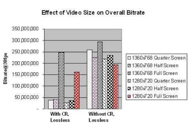
Figure 2.6: Bitrate@30fps comparison of schemes using JPEG-2k, with and without SBB-NR-CR
Rates achieved with and without SBB-NR-CR
This section presents a comparative study of lossless SBB-NR-CR and lossless
encoding without Conditional Replenishment, for 6 different image data sets. Three data
sets are of the same size, but differ in the amount of video data present in them. The data
sets used the ForestFight and LGE video running on the screen along with other activity
on the desktop like reading PDF documents, browsing the Internet etc. The first image set
is of size 1280x720, and the second is of size 1360x768.
It can be seen from Figure 2.6, that using lossless CR gives us better rates, and
consequently bitrates compared to the ones achieved without CR. This happens because
of the high correlation between consequent images, which leads to very small video part of
the image, and thus leads to good overall rate. It can also be seen that as the percentage
of the video portion in the image increases, the margin of advantage that the Conditional
Replenishment scheme had, reduces. These images were sequences that were around 4000
frames, and the rate shown here is the average rate achieved over a typical desktop like
usage with varying proportions of video content on the screen. The video playing on the
screen carried the Forest sequence and the LG sequence. The exact values of the rates
Table 2.2: Rate comparison of schemes using JPEG-2k, with and without CR
ImageSize Input type Compr. Rate Bitrate@30fps Compr. Rate Bitrate@30fps using SBB-NR-CR using SBB-NR-CR CleanImage CleanImage 1360x768 Quarter Screen Video 0.051 38,353,305 0.344 258,696,806 1360x768 Half Screen Video 0.565 42,489,446 0.2984 224,404,439 1360x768 Full Screen Video 0.33 248,168,448 0.388 292,252,188 1280x720 Quarter Screen Video 0.0435 28,864,512 0.33 218,972,160 1280x720 Half Screen Video 0.056 37,158,912 0.354 234,897,408 1280x720 Full Screen Video 0.2411 160,042,106 0.2897 192,231,014
SBB-NR-CR-Lossy-WithoutKeyFrame Vs SBB-NR-CR-Lossless
In this section, we will see the performance of the SBB-NR-CR Lossy scheme in
comparison with SBB-NR-CR-Lossless scheme. Adding Keyframes and lossy SBB-NR-CR
with Keyframes, would still cause the increase in video content as was explained in the
previous section. Exactly how much would it make a difference is not considered in the
thesis and is part of future work. Looking at Table 2.2, for each of the sequences in that
table, we know mean rates achieved by the CR-Lossless. We now subject
SBB-NR-CR-LossyJPEG-2000 to encode at this rate and then measure the PSNRs. As said before,
we are following this methodology, because it is possible to encode lossily at ANY arbitrary
rate, and thus if we wanted to really measure which one of these two schemes is better,
we must see how good/bad the quality of the SBB-NR-CR-Lossy scheme at the rate of the
lossless is. The input data set is the same as was considered in the measurements taken for
Table 2.2, and the following results are observed. Note carefully how the Av. Compr Rate
shown in Table 2.3 is exactly the same compression rate as shown for SBB-NR-CR-Lossless
in Table 2.2. With reference to Figure 1.2 we are referring here to Scheme 23 and Scheme
3.
Table 2.3: PSNR and Bitrate of the Lossy-Video Scheme
ImageSize Input type PSNR PSNR PSNR Av. Compr Bitrate@30fps
(Red) (Green) (Blue) Rate (bps)
1360x768 Quarter Screen Video 29.85 29.85 29.85 0.051 38,353,305 1360x768 Half Screen Video 36.82 37.01 36.45 0.056 42,113,433
1360x768 Full Screen Video 48.13 48.17 48.17 0.33 248,168,448
Thus, by looking at these numbers, we can say now, that if we try doing
SBB-NR-CR-Lossy-WithoutKeyFrame at the same rate at which we try doing SBB-NR-CR-Lossless,
then we achieve quality of images as shown above. Note that the bitrate would be the
same. It can be seen from Table 2.3 that for QuarterScreen Video and HalfScreen video,
the SBB-NR-CR-Lossy scheme performs quite poorly in terms of quality. For Fullscreen
”video” sequences, the quality is sufficiently good, but is still lossy.
Thus, in the preceding sections, we have seen how SBB-NR-CR-Lossless compares
with SBB-NR-CR-Lossy. It can be seen that for QuarterScreen and FullScreen ”Video”
image sequences SBB-NR-CR-Lossless outperforms SBB-NR-CR-Lossy, but for FullScreen
images, SBB-NR-CR-Lossy gives good quality images. Because the goal of the project is to
seek a high-quality scheme, we now drop the idea of SBB-NR-CR-Lossy schemes because we
have seen that for SBB-NR-CR, lossless image encoding performs better than lossy image
encoding on average over different kinds of input images.
2.3
Comparison of JPEG-2000 and JPEG-LS results
2.3.1 Comparison of Compression Rates
It was seen in the previous section that a lossless scheme for doing SBB-NR-CR is
better than a lossy scheme without Keyframes, both in terms of bitrate and quality. This
section will compare the two codecs, JPEG-2000 and JPEG-LS on the basis of bitrates
obtained by each in encoding output of the SBB-NR-CR. Table 2.4 shows the bitrates
obtained for the same input images as in the previous section.
Table 2.4: JPEG-2000 Vs JPEG-LS Bitrates
ImageSize Input type SBB-NR-CR SBB-NR-CR SBB-NR-CR SBB-NR-CR JPEG-2000 JPEG-LS JPEG-LS JPEG-LS
Average Average Minimum Maximum
BitRate@30fps BitRate@30fps BitRate@30fps BitRate@30fps
(bps) (bps) (bps) (bps)
Figure 2.7: Comparison of JPEG-LS and JPEG-2000
Figure 2.7 shows data described in the Table 2.4 in the form of a graph. It can be
seen from the results obtained above, that LS and
SBB-NR-CR-JPEG-2k-lossless are comparable in terms of the bitrates achieved.
2.3.2 Comparison of encoding time
In order to see whether JPEG-LS offers any advantage in terms of encoding time
in comparison with JPEG-2000, we measured the time it took for doing Conditional
Replen-ishment by each method, for a small input sample. Table 2.5 shows the average encoding
time for the text portion and the video portion images, created during the Conditional
Replenishment process.
Table 2.5: JPEG-2000 Vs JPEG-LS Encoding Timings
Image Type Text Enc. Time Vid Enc. Time
Average (sec) Average (sec)
QuarterScreen JPEG-2k 0.888 0.941
QuarterScreen JPEG-LS 0.01804 0.04009
HalfScreen JPEG-2k 0.908 0.941
HalfScreen JPEG-LS 0.01408 0.03999
FullScreen JPEG-2k 0.829 1.218
Fullscreen JPEG-LS 0.01531 0.18733
for our input image sequences.
2.4
Conclusion for SBB-NR-CR
From the previous sections, it was seen that SBB-NR-CR is an effective way to
do video compression. It was seen that depending on the quantity of ”video” data across
images, compression can be achieved ranging from 3 times to 10 times using
JPEG-LS. We also found out for the video sequences that we tested, that
Lossless performs better on average(quality as well as encoding time) than
SBB-NR-CR-Lossy, meaning that we achieve better compression on average for the sequences tested,
doing Non-Residual Conditional Replenishment in a lossless way than doing it in a lossy
way. We also see that the JPEG-LS implementation encodes significantly faster compared
to the JPEG-2k implementation.
As mentioned before, it should be noted at this point that in our
SBB-NR-CR-Lossy scheme we do not test what happens when we insert a key frame after every specific
number of frames. We have only noted that for the data set that we considered, doing
SBB-NR-CR-Lossy-Without-Key-Frame is worse than
SBB-NR-CR-Lossless-Without-Key-Frame. Inserting a key frame and checking the performance has been excluded from the
thesis and remains a task of the future. As mentioned before, the task of the project was
to seek a low bitrate, high quality and computationally lightweight scheme, and because we
have seen that SBB-NR-CR-Lossless gives unmatchable quality, and is better in terms of
bitrate (on average) than SBB-NR-CR-Lossy (even WITH Keyframes), we opt for working
on lossless schemes. We have also seen that lossless image encoding schemes based on
JPEG-LS outperform JPEG-2k in terms of encoding time. As a consequence we will pursue
this thread of doing SBB-NR-CR-Lossless, and attempt to improve on the performance of
Chapter 3
Design of Simple Block Based
Conditional Replenishment
Variants
In the previous chapter we discussed the SBB-NR-CR scheme. In this chapter we
will discuss variants of this scheme, with the goal of attempting to improve the compression
rate. We will discuss the motivations for, and the design of each of the following schemes.
This chapter describes the techniques and the next chapter will discuss the results. These
schemes can be seen in Figure 1.2.
1. CleanImage Lossless Encoding Schemes
(a) CleanImage JPEG-LS: This is also called Motion JPEG-LS.
(b) CleanImage ZLIB: This is also called Motion ZLIB.
2. SBB-NR-CR-Lossless using ZLIB: In this scheme, the ”text” and ”video” image is
encoded using ZLIB. This scheme is similar to Tight-VNC-ZLIB.
3. Non-Residual Lossless Schemes (SBB-NR-CR-Lossless) based on Histogram Packing
(a) CR-OfflineHistogramPacked-JPEG-LS: Image obtained after
SBB-NR-CR subjected to offline Histogram Packing followed by JPEG-LS encoding.
(b) SBB-NR-CR-OnHistogramPacked-JPEG-LS: Image obtained after SBB-NR-CR
(c) SBB-NR-CR-ZLIB: Encoding of both, Video image and Text Image using ZLIB.
(d) SBB-NR-CR-OfflineHistogramPacked-ZLIB: Image obtained after SBB-NR-CR
subjected to offline Histogram Packing, followed by ZLIB encoding.
(e) SBB-NR-CR-OnHistogramPacked-ZLIB: Image obtained after SBB-NR-CR
sub-jected to Online Histogram Packing, followed by ZLIB encoding.
4. Non-Residual Lossy Schemes (SBB-NR-CR-Lossy) with Intra Frame/Key Frame
re-fresh
5. Residual Lossless Schemes (SBB-R-CR-Lossless) based on Longest Prefix Matching
Motion Estimation and Gray Code Variant
(a) SBB-R-CR-LPME-ZLIB: Longest Prefix Matching Motion Estimation (LPME)
using XOR (addition modulo 2), followed by ZLIB encoding of the bitstream.
(b) SBB-R-CR-Gray-LPME-ZLIB: LPME using Gray Codes.
6. Residual Lossless Schemes (SBB-R-CR-Lossless) based on SAD Motion Estimation
and Histogram Packing
(a) SBB-R-CR-SAD-WithSign-JPEG-LS: Simple Block Based, Residual Conditional
Replenishment. The Residual is found out using Motion Estimation with sign,
followed by JPEG-LS.
(b) SBB-R-CR-SAD-WithoutSign-JPEG-LS: Simple Block Based, Residual
Condi-tional Replenishment. The Residual is found out using Motion Estimation
with-out sign, followed by JPEG-LS.
(c) SBB-R-CR-SAD-WithSign-ZLIB: Simple Block Based, Residual Conditional
Re-plenishment. The Residual is found out using Motion Estimation with sign,
followed by ZLIB.
(d) SBB-R-CR-SAD-WithoutSign-ZLIB: Simple Block Based, Residual Conditional
Replenishment. The Residual is found out using Motion Estimation without
sign, followed by ZLIB.
(e) SBB-R-CR-SAD-WithSign-OnlineHistogramPacked-JPEG-LS: SBB-R-SAD-WithSign
JPEG−LS/
(RGB) Current
Image
Tx
Encoder Side
Encoding ZLIB
Figure 3.1: Clean Image Lossless Encoding
(f) SBB-R-CR-SAD-WithoutSign-OnlineHistogramPacked-JPEG-LS:
SBB-R-SAD-WithSign undergoing Online Histogram Packing, followed by JPEG-LS.
(g) SBB-R-CR-SAD-WithSign-OnlineHistogramPacked-ZLIB: SBB-R-SAD-WithSign
undergoing Online Histogram Packing, followed by ZLIB.
(h) SBB-R-CR-SAD-WithoutSign-OnlineHistogramPacked-ZLIB: SBB-R-SAD-WithSign
undergoing Online Histogram Packing, followed by ZLIB.
7. Residual Lossy Schemes (SBB-R-CR-Lossy) with an Intra/Key Frame:
This thesis does not cover these schemes and comparison with the codecs presented
herein, and with its very similar variants such as MPEG-2/H.264 is part of future
work.
3.1
CleanImage Lossless Encoding Schemes
These schemes are characterized by encoding the image directly without subjecting
them to SBB-NR-CR. In this thesis we discuss the following CleanImage encoding schemes.
3.1.1 CleanImage JPEG-LS
In this technique, we do not perform SBB-CR, but rather the original image (called
as Clean Image here) is encoded directly using JPEG-LS. The schematic block diagram is
as shown in Figure 3.1.
3.1.2 CleanImage ZLIB
In this technique, we do not perform SBB-CR, but rather the original image (called
shown in Figure 3.1.
3.2
SBB-NR-CR-ZLIB
In this scheme, the text and the video image as shown in Figure 2.1 are compressed
by the ZLIB compression library. The Flash Screen Video Codec from Adobe is a 16x16
Block Based codec, and the similarity of the performance of SBB-NR-CR-ZLIB with the
performance of the Adobe video codec leads us to guess that Adobe FLV is based on
SBB-NR-CR-ZLIB, but we have no way of verifying because Adove FLV is not an open format.
3.3
Non-Residual Lossless Schemes (SBB-NR-CR-Lossless)
based on Histogram Packing
The basic tool that is used in designing point operations1 (and many other
opera-tions as well) is the Image Histogram. The histogramHg of the digital imagegis a plot or
graph of the frequency of occurrence of each gray level in g2. Hence,Hg is a one-dimensional
function with domain{Imin, ..., Imax}, and range extending from 0 to NM (for the image of
size NxM). The histogram is given explicitly byHg(k) =J if the image g contains exactly
J occurrences of the gray level (Intensity Value) k. The algorithm to compute the image
histogram involves a simple counting of gray levels, which can be accomplished even as the
image is scanned.[15]
In [16], Armando J. Pinho discusses the methods that can be used to improve
the compression performance of lossless compression of images with sparse histograms.
Histogram packing is a known preprocessing method capable of producing improvements in
compression rate if applied prior to lossless compression of images having sparse histograms.
[16] There are two ways of performing this Histogram Packing in the literature, that being
Offline Histogram Packing, and the other being Online Histogram Packing.
Paulo J.S.G and Armando J. Pinho discuss in [17], that the Histogram Packing
method described in [16] can be best understood in terms of its effect on the total image
1
Image Processing Operations that are applied to individual pixels/pels
2
variation. The packing transformation reduces the total variation in the image, yielding a
smaller variation that is easier to compress. We now discuss these two schemes:
3.3.1 Offline Histogram Packing
Offline Histogram Packing is obtained through the construction of an one-one
order preserving mapping, h, from the image intensity values, I, into a contiguous subset
of N0. Let the range of the intensityI in the image g, beImin to Imax. Further, letIα0 be
the smallest image intensity value that has non-zero occurrence in the image g, Iα1 be the
second smallest intensity has non-zero occurrence in the image g and in general Iαi be the
ithsmallest intensity value with an occurrence non-zero number of times in g, andI
αN−1 the
highest such intensity. If the image is made up of more than one component, then this same
method is applied to every component separately. It suffices to describe the algorithm for
just 1 component, because we can apply the same method for every component separately.
The mappingh from non-zero intensities toN0 is as follows:
h= (Iα0 7→0, Iα1 7→1, Iα2 7→2, I2 7→2, ..., IαN−2 7→N−2, IαN−1 7→N −1) (3.1)
Thus, when this mapping is applied to an image g, a new image gof hp =h(g) is obtained
which is more compression friendly thang [16].
In order to apply the mappingh to an imageg, we must need to know apriori the
histogram of the image. In this implementation, Offline Histogram Packing is done in a
two-pass process. The first two-pass creates the histogram of the image g for each channel present
in the image (In our case it is, R, G, and B), and the second pass packs the histogram using
the mapping h for each channel. At the end of this process, we have an image gof hp i.e. g
after Offline Histogram Packing (ofhp), that has total variance less than that ofg. [17]
Note that this mapping needs extra side information for the inverse mapping. The
inverse function is needed to be computed in order to reconstruct the original image from
the histogram packed image. One way this mapping functionhcan be reversed is by
build-ing a map of the histogram as it existed before the Histogram Packing. For every image
intensity Ij, where Imin≤Ij≤Imax, that exists in a component c of an image g, we mark a
’1’ in the mapping, and all the intensities that are not present are marked with zero. We
f(Ij) = 0 if NumOccur(Ij=0)
= 1 if NumOccur(Ij6=0) ∀Imin≤Ij≤Imax
Once the decoder has this mapping f(·), as soon as it starts reconstructing the
image, for every intensity that it sees in the histogram packed image, all it needs to do
is to interpret this intensity Ik, as the Ikth smallest value from Imin with a non-zero bin
count, in the original histogram before Histogram Packing. Thus, if the decoder sees a ’3’
as an example, it should check f(·) to find the 3rd smallest element with a nonzero bin, and
substitute that intensity value instead of the 3.
3.3.2 Online Histogram Packing
Offline Histogram packing assumes an apriori knowledge of the image histogram
before the packing process begins. As has been noted before, this can mean doing a one-pass
over the entire image and build the histogram. An alternative technique called Online
His-togram Packing has been proposed by Armando Pinho in [18]. Similar to Offline HisHis-togram
Packing, this is also a preprocessing method, which has a variance reducing property. In
[18], Pinho demonstrates that this method can give better performance than Offline
His-togram Packing when used with JPEG-LS. The preprocessing technique can be explained
as follows:
Let us assume that the preprocessor is going to handle sample xt, and that it
has already found n different intensity values given byIt = I
0, I1, I2, ..., In−1. Let us also
assume, without loss of generality, thatIi < Ij,∀i<j. Then the intensity mapping, ht, that
is used to map thekth smallest sample I
k is given by:
ht= (I07→0, I17→1, I2 7→2, I2 7→2, ..., Ik 7→k, In−17→n−1) (3.2)
which maps ascending sorted intensity values into ascending sorted contiguous indexes. If
xt ∈It, then symbolht(xt) is generated by the preprocessor. On the other hand, ifxt∈/ It,
then the symbol that is generated by the preprocessor isn, i.e. the value that is not present
in the mapping table so far. In this case, this new intensity value is recorded. When the