ABSTRACT
ZHOU, CHUNDA. DNA Manipulation in Microfluidic Devices. (Under the direction of Robert Riehn.)
Since the discovery of DNA structure in 1953, DNA drew broad attention from both biology
and medical care fields. DNA manipulation became an important field of investigation, and the
behavior and properties of DNA have been studied extensively. However, in electric field the
behavior and properties of DNA are still controversial. The study of manipulating DNA with
electric fields not only supplies tools for sequencing technologies but also contributes to the
building of theoretical framework of polyelectrolytes in general which will, in turn, advance the
applications.
In our experiments, we discovered a novel behavior of DNA under alternating electrical fields.
We observed that DNA collapses under an alternating electric field in different environments.
This is in contrast to the predictions of conventional polyelectrolyte theories. This means that
the traditional theories may need be changed or at least revised. Two models are proposed
to describe the collapse phenomenon for two limiting conditions. A computer simulation was
also carried out in order to investigate which physical processes are required for a contraction
under an a.c. field. The preliminary result has shown a qualitative agreement with experiment
observation.
We also developed a method for the dissection of C. elegans embryos and isolated murine
cells. By using a pulsed UV laser optical system, we are able to cut membranes of C. elegans
embryos and membranes of BAF/3 cells open. Further, with the help of a microfluidic control
system, we were able to isolate generic DNA from the cytoplasm, a necessary step for DNA
© Copyright 2012 by Chunda Zhou
DNA Manipulation in Microfluidic Devices
by Chunda Zhou
A dissertation submitted to the Graduate Faculty of North Carolina State University
in partial fulfillment of the requirements for the degree of
Doctor of Philosophy
Physics
Raleigh, North Carolina
2012
APPROVED BY:
Keith Weninger Melissa Pasquinelli
Shuang Fang Lim Robert Riehn
BIOGRAPHY
If you could go back to A.D. 1996, planet: Earth, 41°35’ N, 120°27’ E and find the author (whose
name in local characters is shown in the picture below), please tell him to let his mother do
careful physical examination every year from then on. The author may be able to make this
ACKNOWLEDGEMENTS
TABLE OF CONTENTS
LIST OF TABLES . . . vi
LIST OF FIGURES . . . vii
Chapter 1 Introduction . . . 1
1.1 Basic polymer physics . . . 1
1.1.1 The ideal chain . . . 1
1.1.2 The non-ideal chain model . . . 2
1.1.3 Radius of gyration . . . 4
1.1.4 Properties of neutral polymers . . . 7
1.2 Polymer dynamics . . . 11
1.2.1 Rouse model . . . 11
1.2.2 Zimm theory . . . 14
1.3 Polyelectrolytes . . . 17
1.4 DNA structures and properties . . . 17
1.4.1 Characteristics lengths of polyelectrolyte in salt solution . . . 21
1.4.2 Studies on DNA properties . . . 24
1.4.3 Polyelectrolytes interact with electric fields . . . 24
Chapter 2 Methods . . . 27
2.1 Experimental methods . . . 27
2.1.1 Micro-channel design and fabrication . . . 27
2.1.2 Biological materials . . . 36
2.1.3 Experiment setup . . . 37
2.1.4 Statistics and error estimation . . . 58
2.2 Simulation methods . . . 60
2.2.1 Bead-spring chain polymer backbone . . . 61
2.2.2 Electrostatics . . . 61
2.2.3 Fluidics . . . 63
Chapter 3 Experimental investigation of DNA in electric field . . . 66
3.1 Basic effect . . . 66
3.2 Frequency and salt dependence . . . 71
3.3 Center of mass motion correction . . . 72
3.4 Dependence on polymer size . . . 90
3.5 Comparison to collapse in nanochannels . . . 93
3.6 Discussion . . . 97
Chapter 4 Computer simulation. . . .103
4.1 System configurations . . . 103
4.1.1 Basic configuration . . . 103
4.1.3 Electrostatic parameters . . . 107
4.1.4 Fluidics parameters . . . 114
4.2 Results and discussion . . . 116
4.3 Conclusions . . . 129
Chapter 5 Pulsed UV laser microdissection . . . .130
5.1 Background . . . 130
5.2 Microchannel design . . . 132
5.3 Microfluid control system . . . 134
5.4 Optical system . . . 135
5.5 Control system . . . 138
5.6 Result . . . 141
Chapter 6 Conclusions and outlook . . . .143
6.1 Conclusions . . . 143
6.2 Potential influence . . . 144
6.3 Possible Applications . . . 144
6.4 Possible future work . . . 145
References. . . .146
Appendix . . . .152
LIST OF TABLES
Table 2.1 Measured Ionic Strength (I) of TBE Buffers [34]. . . 36
Table 4.1 Comparison between four simulation scenarios. . . 107
Table 4.2 Parameters for fludics. . . 115
Table 4.3 Results of four simulation scenarios. . . 119
Table 4.4 Comparison of average ion densities in the 0 to 10 spatial range between different scenarios. . . 125
LIST OF FIGURES
Figure 1.1 Lattice model for ideal chain. The b vectors are the basis of the lattice. White dots are polymer segments. While the thick lines connecting them are bonds [21]. . . 3 Figure 1.2 The bending of a small polymer segment ∆l.~e(l) represents the tangential
vector at the location l [76]. . . 8 Figure 1.3 Log-log plot of the mean square displacement of the terminal segment
of a DNA molecule, shown in solid line. The dashed line is the result calculated by using Zimm’s theory [52]. . . 16 Figure 1.4 Space-filling model of the double helix [83]. . . 18 Figure 1.5 Chemical structure of double strand DNA molecule and the base paring
rule [83]. . . 19 Figure 1.6 Chemical structure of four bases [83]. . . 20 Figure 1.7 Electrical double layer around DNA molecules [69]. . . 21 Figure 1.8 Schematic of the macroion shape change in electric field. (a) is the ellipsoid
macroion. (b) is the elongated ellipsoid macroion. . . 25
Figure 2.1 Micro-channel chip layout. (a) the layout for the whole chip. (b) the cen-tral constriction. (c) the fork structure. . . 28 Figure 2.2 Photoresist thickness vs. spin speed of S1800 photo resist [1]. . . 30 Figure 2.3 Chip with reservoirs. . . 31 Figure 2.4 FEA simulation of electric field in micrhochannel. The top panel shows
the section along center of channel. The bottom panel shows overall field landscape. . . 33 Figure 2.5 FEA simulation of electric field in microchannel constriction region. . . . 35 Figure 2.6 Chemical structure of YOYO-1 iodide [62]. . . 37 Figure 2.7 Absorption and fluorescence emission spectra of YOYO-1 bound to DNA
and filter set spectrum [62]. . . 38 Figure 2.8 Schematic diagram of fluorescent microscope [2]. . . 39 Figure 2.9 The schematic of dichroic filter set [2] . . . 40 Figure 2.10 The spectra of dichroic filter set we used. (http://www.semrock.com) . . . 41 Figure 2.11 Schematic of the optical system for DNA in alternating electric field
ex-periments. (a) a lens which could easily be flipped in and out of the beam path. (b) a lens whose position is adjustable along the beam path during the experiment. (c), (d) and (e) are lenses belong to the microscope. . . . 43 Figure 2.12 Steering mirrors and servo motors. (a) the schematic of the steering
mir-rors. (b) the schematic of the light spot in the illumination field. (c) the real steering mirrors. . . 44 Figure 2.13 Structure of Labview-FPGA based control system. . . 46 Figure 2.14 Triangle wave steering mirror control signal. . . 47 Figure 2.15 Sequence diagram of illumination laser and steering mirror position
Figure 2.16 Single DNA molecule image, shown in 3-D plot (pseudo color). . . 50 Figure 2.17 Single DNA molecule image (pseudo color). . . 52 Figure 2.18 “Mask” pattern generated based on a single DNA molecule image. . . 52 Figure 2.19 A single DNA molecule image operated by a “mask” pattern (pseudo color). 53 Figure 2.20 The block diagram of a PID controller [3]. . . 55 Figure 2.21 Simulation of the behavior of a closed-loop system with proportional
control. The set point is 1 and the transfer function of the system is
G(s) = (s+1)1 3. The upper graph shows the output value y for different gains K. The lower one shows the control signal for different gains [32]. . . 55 Figure 2.22 Simulation of the behavior of a closed-loop system with proportional and
integral control. The set point is 1 and the transfer function of the system is G(s) = (s+1)1 3. The controller gain K is 1. The upper graph shows the output value y for different integral time Ti. The lower one shows the
control signal for different integral time [32]. . . 56 Figure 2.23 Simulation of the behavior of a closed-loop system with proportional,
in-tegral and differential control. The set point is 1 and the transfer function of the system is G(s) = (s+1)1 3. The controller gain K is 3, and the inte-gral timeTi is 2. The upper graph shows the output value y for different
derivative times Td. The lower one shows the control signal for different
derivative time [32]. . . 57 Figure 2.24 The schematic of PID control system. . . 58 Figure 2.25 The schematic simulation methods for different length and time scales of
the system [47]. . . 60 Figure 2.26 The D3Q19 lattice geometry. . . 63
Figure 3.1 Images of λ-DNA in alternating electric fields at 300 Hz. (A) shows the DNA molecule fluctuates freely before alternating electric field was ap-plied. (B) shows the DNA molecule fluctuates under relative weak al-ternating electric field (∼24.33kV/m). In both groups, individual frames were acquired with a 0.7 s interval, and the number indicates the relative order. . . 67 Figure 3.2 Images of λ-DNA in alternating electric fields at 300 Hz. (C) shows the
DNA molecule collapses at∼66.44 kV/m. (D) shows the molecule changes shape along the electric field direction (vertical direction in these pic-tures) under high electric field (∼122.35kV/m). In both groups, individ-ual frames were acquired with a 0.7 s interval, and the number indicates the relative order. . . 68 Figure 3.3 Radius of gyration changes with electric field strength in 2×TBE and
300 Hz electric field. Each black square in the same electric field strength represents a molecule. . . 69 Figure 3.4 Anisotropy as function of strength in 2×TBE and 300 Hz electric field.
Figure 3.5 Radius of gyration as function of electric field strength and driving fre-quency in 0.25×TBE. Curves for different frequencies are separated by a 0.3 µm offset. . . 73 Figure 3.6 Radius of gyration as function of electric field strength and driving
fre-quency in 0.5×TBE. Curves for different frequencies are separated by a 0.3 µm offset. . . 74 Figure 3.7 Radius of gyration as function of electric field strength and driving
fre-quency in in 1×TBE. Curves for different frequencies are separated by a 0.3 µm offset. . . 75 Figure 3.8 Radius of gyration as function of electric field strength and driving
fre-quency in 2×TBE. Curves for different frequencies are separated by a 0.3
µm offset. . . 76 Figure 3.9 Center of mass blurring effect, schematic. . . 77 Figure 3.10 Illumination power density distribution for harmonic motion along the
electric field direction. . . 79 Figure 3.11 Image pattern due to center of mass motion. (A) is the computer
sulation of the illumination pattern (pseudo color). (B) is a typical im-age taken from experiment forlambda-DNA in 2XTBE and 146.82kV/m, 100Hz driving a.c. electric field. . . 81 Figure 3.12 Linear fit of the linear region of the radius of gyration vs. electric field in
2×TBE at 300Hz. . . 82 Figure 3.13 Radius of gyration as function of electric field strength in 0.25×TBE after
correction. Each curve is shifted by a 0.3 µm offset. . . 83 Figure 3.14 Radius of gyration as function of electric field strength in 0.5×TBE after
correction. Each curve is shifted by a 0.3 µm offset. . . 84 Figure 3.15 Radius of gyration as function of electric field strength in 1×TBE after
correction. Each curve is shifted by a 0.3 µm offset. . . 85 Figure 3.16 Radius of gyration as function of electric field strength in 2×TBE after
correction. Each curve is shifted by a 0.3 µm offset. . . 86 Figure 3.17 Laser flash sequence and center of mass harmonic motion under 100Hz
driving a.c. field. The three harmonic motions are with an initial phase of 0, 78 ×2π, 68 ×2π, respectively. . . 88 Figure 3.18 Critical electric field strength vs. electric field frequencies. . . 89 Figure 3.19 Radius of gyration of T4-DNA as function of electric field strength in
2×TBE at 300Hz driving frequency. . . 91 Figure 3.20 Radius of gyration of T4-DNA as function of electric field strength in
2×TBE at 300 Hz driving frequency, after correction for the center of mass motion. . . 92 Figure 3.21 Normalized relative radius of gyration of T4-DNA in 2× TBE. . . 94 Figure 3.22 Fractional extension vs. electric field forλ-DNA in different nanochannels
in 0.5×TBE. . . 96 Figure 3.23 Critical electric field strength vs. electric field frequencies forλ-DNA in
Figure 3.24 Schematic of loosely bound model. . . 99
Figure 3.25 Schematic of tightly bound model. . . 100
Figure 4.1 Schematic diagram of simulation configuration of scenario 1. . . 104
Figure 4.2 Schematic diagram of simulation configuration of scenario 2. . . 105
Figure 4.3 Schematic diagram of simulation configuration of scenario 3. . . 105
Figure 4.4 Schematic diagram of simulation configuration of scenario 4. . . 106
Figure 4.5 Force versus extension data (red crosses) for λ-phage dsDNA (48,502 bp) pulled by magnetic beads in 10 mM Na+ buffer[72]. The data are fit to a WLC model solved numerically (WLC exact) or using Equation 3 in [15] (WLC interpolated), both assuming P = 53 nm. The FJC curve assumes b = 2P = 106 nm. [15] . . . 108
Figure 4.6 Center of mass motion of the polymer chain in three directions under an a.c. electric field. Note the electric field is applied in z-direction. . . 110
Figure 4.7 Ion relaxation simulation scenario. Cations and anions were placed in two planes 0.4×320 away, initially. . . 111
Figure 4.8 Cation number in the slit changes with time. . . 113
Figure 4.9 The radius of gyration changes with time (scenario 2). . . 114
Figure 4.10 The autocorrelation of the radius of gyration changes with time (scenario 2). . . 115
Figure 4.11 The semilogarthmic plot of autocorrelation of the radius of gyration and eq. 4.8. . . 116
Figure 4.12 Rg vs. time in scenario 1 and scenario 2. . . 117
Figure 4.13 Rg vs. time in scenario 1, scenario 3 and scenario 4. . . 118
Figure 4.14 The schematic of bead-spring polymer chain and the Gaussian pulses created to represent it. . . 121
Figure 4.15 The semilogarthmic plot of power spectrum of scenario 1. . . 122
Figure 4.16 The semilogarthmic plot of power spectrum of scenario 2. . . 123
Figure 4.17 Schematic of ion density distribution calculation. . . 124
Figure 4.18 The coion density distribution in scenario 1, (A) and scenario 2, (B). . . . 126
Figure 4.19 The counterion density distribution in scenario 1, (A) and scenario 2, (B). 127 Figure 4.20 The center of mass coordinate in z direction of ions in scenario 1. . . 128
Figure 4.21 The center of mass coordinate in z direction of ions in scenario 2. . . 128
Figure 5.1 Rat cell interact with laser created tandem,[68]. . . 131
Figure 5.2 The central crossing part layout of the micro-channel chips. . . 132
Figure 5.3 Analysis flow: embryo, cell and genome DNA. . . 133
Figure 5.4 Comparison of image and the schematic. . . 133
Figure 5.5 Schematic of the tubing and the flow profile. . . 134
Figure 5.6 Syringe pumps and the control program. . . 136
Figure 5.7 Schematic of the gravity fluid control. . . 136
Figure 5.8 UV laser microdissection optical system schematic diagram. The blue block represents the microscope. . . 137
Figure 5.10 Schematic of the alignment. The two lines shows the cutting paths of the UV spot before and after the alignment. . . 140 Figure 5.11 C. elegans embryo microdissection. The diameter of C. elegans embryo
shown here is about 20µm. . . 141 Figure 5.12 Ba/F3 cell microdissection. The diameter of Ba/F3 cell shown here is
Chapter 1
Introduction
1.1
Basic polymer physics
1.1.1 The ideal chain
A considerable number of phenomena in polymer physics can be explained using extremely
general models, which are applicable to most existing polymers. A polymer is a linear chain of
repeated units (monomers). A typical polymer contains over 100 of these monomers, which is
expressed by saying that the degree of polymerization is greater than 100. As a result, in most
cases, the number of configurations of a polymer molecule is enormous. In order to evaluate
properties of polymers, statistical methods are used as the tools.
In the simplest possible model, the polymer is represented as a collection of stiff rods that
are freely jointed. Consider that each polymer molecule consists of N identical segments. Each
segment is represented by a vector ~r. Its length r = b. Also define R~ as “end-to-end” vector
which can be expressed as
~ R=
N
X
i=1
~ri (1.1)
Assume each segment oriented randomly,h~rii= 0. Then the average
D
~ R
E
is also zero. Thus,
it can not be used to evaluate the size or spacial distribution of segments. As a result,
D
~ R2
E
calculated
D
~ R2E=
N X i=1 N X j=1
h~ri·~rji (1.2)
If i6=j,h~ri·~rji= 0. Thus
D ~ R2 E = N X i=1
~r2i =N b2 (1.3)
The “end-to-end” vector distribution probability,P(R, N~ ), is used to generate further statistical
properties. For very long polymers, e.g. N 1, the central limit theorem dictates that the probability of finding a given P(R, N~ ) is a Gaussian. For our collection of steps with constant
length it can be expressed by the following expression
P(R, N~ ) = ( 3 2πN b2)
3/2exp(− 3R~2
2N b2) (1.4)
Since the distribution is isotropic, we can neglect the direction of R~. Define W(R) as a
radical configuration distribution density, so that W(R)dR is the total number of polymer
configurations when one end of the polymer lies betweenR and R+dRfrom the origin. With
the help of eq. 1.4, it can be expressed as
W(R) = 4πR2
3 2πN b2
3/2
exp
− 3R 2
2N b2
(1.5)
1.1.2 The non-ideal chain model
A more careful examination of the previous model shows a problem: the assumption that each
segment has completely random distribution is unphysical–different segments can’t occupy the
same space simultaneously. As a result, a finer model is built which includes the influence of
the volume which is excluded from the phase space of a second segment by the presence of a
first segment. The influence of this excluded volume effect can be studied by assuming that the
polymer is restricted to occupy the nodes of a lattice Figure 1.1.
Figure 1.1: Lattice model for ideal chain. The b vectors are the basis of the lattice. White dots are polymer segments. While the thick lines connecting them are bonds [21].
the polymer segments as a gas, the probability of overlap between any two segments is vexclude
R∗03 ,
wherevexclude represents the volume of each lattice element which can only be occupied by one
polymer segment due to excluded volume effect. The likelihood that a chain configuration has
no overlap is thus dictated by the number of possible combinations of piking two rods without
overlap, and the total probability of finding no overlap is
P(R∗0) =
1−vexclude
R∗03
N(N−1)/2
(1.6)
For N 1 we expect vexclude/R3 1, and the approximation
P ≈exp
−N 2v
exclude
2R∗03
(1.7)
can be made. We now assume that the scale of the sphere within which all monomers are
use the probability correction in eq. 1.5, which is changed into
Wexclude(R) =W(R)P(R) = 4πR2
3 2πN b2
3/2
exp
− 3R 2
2N b2 −
N2v exclude 2R3
(1.8)
The R for maximum value of configuration probability distribution is obtained by taking
the derivative of eq. 1.8 and demanding that it equals 0. We obtain (approximately)
0 =
1− R 2
m
N b2 +
N2vexclude
R3
m
(1.9)
It is informative to consider the relative size of the coil with and without excluded volume
interaction. We find
N12vexclude
b3 =
Rm R0 5 − Rm R0 3 (1.10)
where R0 = √N b. For sufficiently large coils the second term on the right side becomes in-significant, and we find that the volume of a coil with excluded volume is in general larger than
without. We also find that the fifth power of that ratio is proportional to the square root of
the degree of polymerization. For determining the explicit dependence of R on the molecular
geometry of the polymer we use Onsager’s argument that finds thatvexclude 'b2w, wherew is the physical diameter of a polymer link.
Rm'(N b)3/5(wb)1/5 =L3/5(wb)1/5 (1.11)
whereLis the length of the polymer were it completely extended. Despite its apparent
simplic-ity, this argument is surprisingly good. For large polymers, the Rm has been shown to be Lν,
ν ≈0.588 in both experiment and renormalization group theory [21].
1.1.3 Radius of gyration
the polymer. We will explain our calculation of the radius of gyration below, starting with a
discrete model of the polymer. An integral expression for a continuously curving molecule gives
comparable results. The radius of gyration is defined as the mean distance between any two
monomers of the molecule
R2g = 1 2N N X i=1 N X j=1
(~ri−~rj)2=
1
N
N
X
i=1
(r~i−~rcm)2 (1.12)
wherer~i is the location of the ith particle and~rcm = N1 PNi=1r~i is the center of mass location.
While one can calculate the radius gyration directly, we have chosen an alternative route based
on the tensor of gyration.
For a given group of particles of a given molecule, the gyration tensor S is defined as the
second moments of the position of each particle. If the radius of gyration is evaluated based
upon a two dimensional image, e.g. a projection of a polymer on a plane, the gyration tensor
is a 2 by 2 matrix with the following element:
Smn =
1
N
N
X
i=1
rm(i)rn(i) (1.13)
where, N denotes for the total number of particles andrm(i),rn(i) denote the Cartesian
coor-dinates of ith particle in the center of mass frame. In fact Smn is symmetric positive definite
matrix [51]. This kind of matrices have following properties:
1. Eigenvalues and eigenvectors exist and the eigenvalues are all positive. We let those be
λx2 and λy2
2. There exists a coordinate system in whichSmn has diagonal form. The diagonal elements
are eigenvalues.
3. Transformation into that coordinate system is a rotation operation. The eigenvalues and
Naturally, if S diagonal then
T r(S) =
N
X
i
(˜x2i + ˜yi2) =λx2+λy2 (1.14)
where ˜xi and ˜yi denote the coordinates of ith particle in the new coordinate (also center of
mass system). The first expression coincides with one of the two equivalent definitions of the
radius of gyration if the coordinates are measures in a center of mass system. We have thus
shown that the sum of the eigenvalues ofS is R2g [78].
Rg2=λx2+λy2 (1.15)
The benefit of using the eigenvalues of the gyration tensor to calculate radius of gyration is
that we can define another important parameter which reflects the configuration or orientation
of the molecule–anisotropy.
Anisotropy= |λx 2−λ
y2|
Rg2
(1.16)
This anisotropy is not accessible using the direct definition or the taking of the trace ofS. To
understand the meaning of this anisotropy, it is instructive to investigate physical significance
of eigenvalues and eigenvectors. Similar to the moment of inertia, in this 2-d case, eigenvalues
of a given molecule denote for the length of major and minor axis of a ellipse shape uniform
mass who has the same second moments as the observed molecule. The two eigenvectors, thus,
denote for the directions of these axis. Therefore, the eigenvalues and eigenvectors represent
the elongation and orientation of the observed molecule.
In our experiments, usually, the position of each particle in the polymer is unknown
(al-though some groups have shown methods to find the configuration approximately). As a result,
eq. 1.13 can not be calculated directly. Instead, the intensity distribution is obtained. Assume
the intensity I, at a given position on a 2-d polymer projection is proportional to the density
have the following relations:
N = X
(m,n)∈A
ρmn
= 1
a
X
(m,n)∈A
Imn (1.17)
Smn =
1
N
X
(m,n)∈A
ρmnrm(i)rn(i) (1.18)
Thus, the gyration matrix can be expressed as
Smn=
1
P
(m,n)∈AImn
X
(m,n)∈A
Imnrm(i)rn(i) (1.19)
In our experiment, the minimum spatial unit is one CCD pixel. The summation thus denotes
for the summation of all the pixels in the observed area.
1.1.4 Properties of neutral polymers
Except for the common model which describes the common properties of different polymers,
internal structures of different polymers do affect overall performance of polymers beyond a
critical length scale. Define the contour length as total length of the curve polymer, denoted by
lcontour. Assume the polymer is a continuous object rather than discrete model shown in the
previous subsection, the “end-to-end” vectorR~ can be expressed:
~ R=
Z lcontour 0
~e(l)dl (1.20)
where~e(l) is the tangent vector of the polymer at the locationl, (Figure 1.2).
The bending property of a polymer can be evaluated by a characteristic length, persistence
length (lpersistence). Define Kcorrelation(∆l) =h~e(l)·~e(l+ ∆l)i, this characteristic length can be expressed as:
lpersistence =
Z ∞
0
Figure 1.2: The bending of a small polymer segment ∆l.~e(l) represents the tangential vector at the locationl [76].
In the absence of other effects, and in thermodynamic equilibrium, an exponential form of
Kcorrelation is chosen,
Kcorrelation(∆l) = exp
− ∆l
lpersistence
= hcos(θm)i
≈ 1−θm 2
2 (1.22)
(1.23)
For a neutral polymer without electrostatic self-interaction having a bending modulus Eb,
the energy to bend the end of a ∆l segment to degreeθm is
U(∆l) = 1 2Eb
θm
∆l
2
∆l (1.24)
We now assume here that the polymer is interacting with surrounding solvent, and that the
energy attributable in the lowest bending mode is the thermal energy kBT (12kBT each for the
T.
lpersistence =
Eb
kBT
(1.25)
Following from the local correlation of tangential vectors, the ensemble average of the
“end-to-end” vector squared R~2 can be expressed as
D
~ R·R~
E
=
Z lcontour 0
Z lcontour 0
~e(l)·~e(l0)dldl0
= 2lpersistencelcontour−2l2persistence
1−exp
− lcontour
lpersistence
(1.26)
In the limit of a large polymer (e.g.lcontourlpersistence), this becomes similar to the expression we found for a freely jointed chain withb= 2lpersistence. This specific length is called the Kuhn
length, lK = 2lpersistence. It gives a boundary beyond which segments of neutral polymers are
considered to be free [25] [26] [66] [75].
At a larger scale than a few Kuhn lengths, the random walk configuration shows the same
statistical properties as a freely jointed chain. Considering the ideal chain lattice model with
its normalized distribution probability
P(R, N~ ) = R∞Ω 0 Ωd ~R
(1.27)
where Ω is the total configuration number of a given polymer, the entropy is expressed as
S = kBlnΩ
= kBlnP(R, N~ ) +kBln
Z ∞
0 Ωd ~R
= 3kBR~ 2
2N b2 +S0 (1.28)
polymerization of a polymer is fixed. The free energy is,
f = U −T S
=− 3kBT ~R 2
2N b2 +f0 (1.29)
We conclude that a force is needed to deform this molecule
~
F = ∂f
∂ ~R
= −3kBT ~R
N b2 (1.30)
This force is obviously linear with extension, but is apparently only applicable around the
equilibrium configuration. Although we only accounted for the entropy contribution, a similar
linear force law can be found based on the partition function of the chain with self-exclusion. In
its nature the resulting force is similar to the pressure the gas in a enclosed container exerted
on the walls of the container. The external force acts against the increase of its entropy.
The non-linear nature of the force when the chain is stretched far beyond its free
equi-librium configuration have been explored widely for DNA. Experiments have shown that the
force-extension curve becomes non-linear when the extension increases beyond a region as is
shown in [59] [8] [60] [15]. In the non-linear regime, not only the random walk statistics but also
the intrinsic mechanical properties, e.g. elasticity caused by the bonds between monomers
con-tribute. Marko and Siggia [50] have shown an interpolation of the elasticity of worm-like-chain.
F lpersistence
kBT
= 1 4
1− R
1.2
Polymer dynamics
1.2.1 Rouse model
The motion of a small particle in solution can be described by a modified Langevin equation in
each coordinate [21] [64]:
dx dt =−
1
ζ ∂U
∂x +g(t) (1.32)
This equation lacks the inertial term and is thus only valid on time scales long compared to
the hydrodynamic damping time. It includes drag force from fluid (−1ζ∂U∂x term) and Brownian
motion (g(t) term), whereζ is the viscous friction constant and U is a potential. The mean of
the Brownian motion term thus has the form
hg(t)i = 0 (1.33)
g(t)g(t0)
= 2Dδ(t−t0) (1.34)
whereDis the diffusion constant, andδ is Dirac delta function. Einstein’s relation linksDand
ζ:
D= kBT
ζ (1.35)
Assume the polymer is a string of N beads connected with identical N−1 linear springs, then the potential of each “interior” bead becomes
U = 1
2k(~rn+1−2~rn−~rn−1) 2
Replacing thex in eq. 1.32 with a three dimensional vector~rn for the position ofnth bead, we
get
d~rn
dt =− k
with the boundary conditions
d~r0
dt = −
k
ζ(~r1−~r0) +~g0(t) d~rN
dt = −
k
ζ(~rN−1−r~N) +~gN(t) (1.37)
This was first proposed by P.E. Rouse.
We can separate independent modes by using normalized coordinates
~ Xp(t) =
1 N Z N 0 dncos pπn N ~
r(n, t) (1.38)
wherep= 0,1,2, . . . . Note the position vector of each bead~rn(t) can be expressed as
~
rn(t) =X~0(t) + 2
∞ X p=1 cos pπn N ~
Xp(t) (1.39)
which is the Fourier series of the motion.
Then eq. 1.36 changes to
d ~Xp
dt =− kp
ζp
~
Xp+~g(t) (1.40)
where ζ0 =N ζ,ζp = 2N ζ for p = 1,2,3, ..., kp = 2p
2π2k
N =
6π2k BT
N b2 with help of eq. 1.30. The Brownian motion term~gp has the following relationship between different modes (pandq) and
different beads (aand b)
gpa(t)gqb(t0)
= 2δpqδab
kBT
ζp
δ(t−t0) (1.41)
whereδpq and δab are Kronecker delta function.
The fundamental mode
~ X0(t) =
1
N
Z N
0
dn~rn(t) (1.42)
of the polymer thus is
D
(X~0(t)−X~0(0))2
E
= 6kBT
N ζ t (1.43)
That is to say the center of mass diffuses with a diffusion constant
D0 =
kBT
N ζ (1.44)
The correlation between normalized coordinates of general modes and beads is
D
~
Xpa(t)X~qb(0)
E
=δpqδab
kBT
kp exp −t τp (1.45)
whereτp = ζkpp = ζN
2b2 3π2k
BT p2. This is remarkable since it predicts that the collective Rouse modes are eigenmodes of the fluctuation spectrum.
The autocorrelation of the end-to-end vector R~ thus can be expressed as a combination of
these eigenmodes:
D
~
R(t)R~(0)E=N b2 X
podd 8
p2π2 exp
−t
τr
(1.46)
The correlation function is expressed as a summation over a series of modes which decay
expo-nentially with different coefficients and characteristic time scales τp. Inspection shows that the
first term has the highest amplitude and longest relaxation time. Thus, the first term has the
biggest contribution. Its relaxation time τ1= ζN 2b2 3π2k
BT is called rotational relaxation time. From eq. 1.30, it is also linked to the Hooke’s constant of a polymer in the linear elasticity
regime.
τ1 =
ζ
k (1.47)
However, the Rouse model doesn’t agree with experimental results for free coils, because it
doesn’t include hydrodynamic interactions. In environments where hydrodynamic interactions
1.2.2 Zimm theory
The effect of hydrodynamic interaction is that each segment of the polymer creates a flow which
influences the motion of others. For the bead-spring model again, eq. 1.36 then is modified into
d~rn
dt =
X
m
~ ~
Hnm·(k(~rm+1+~rm−1−2~rm) +~gm(t)) (1.48)
whereH~~nmis called Oseen tensor. It connects the motion of different beads with a hydrodynamic
interaction that is principally a Stokes flow.
~ ~ Hnn =
~ ~ I ζ and ~ ~
Hnm =
1 8πηrnm
~ rnm~rTnm
r2
nm
+I~~
(1.49)
whereI~~is the identity matrix,η is the viscosity of the solvent and~rnm is the vector from bead
nto bead m.
In order to simplify the nonlinear equation eq. 1.48, Zimm used a preaveraging approximation–
replace theH~~nm with its equilibrium average value
~ ~ Hnm eq
[87]. In θ solution (the polymer
acts as an ideal chain), ~rnm has a Gaussian distribution with a variance of |n−m|b2. As a
result, the tensor can be expressed as
~ ~ Hnm eq = ~ ~ I p
6π3|n−m|ηb (1.50)
Thus, eq. 1.48 can be converted into a form similar to eq. 1.36. Using the same technique
used there, we can again get the center of mass diffusion constant and rotational relaxation
D0 =
8kBT
3 √
6π3η√N b
and
τr =
η(√N b)3 √
3πkBT
≈ 0.325η( √
N b)3
kBT
. (1.52)
When excluded volume effect is considered, the chain statistics are perturbed and these
parameters are modified in a fashion similar to the radius of the coil [22]
D0∼
kBT
ηN3/5b (1.53)
and
τr∼
η(N3/5b)3 √
3πkBT
. (1.54)
The Rouse model, the Zimm model in a ?-solvent and the Zimm model of a self-avoiding
chain in a good solvent clearly show different dependencies. For the Rouse model, the drag
coefficient ζ depends on the polymerization, N of the polymer. That means the shape of the
molecule does not affect its behavior under a flow, but only the stored contour length does.
However, in Zimm’s theory, the ζ ∼ Nnvb ∼Rg reveals the shape dependency by linking the
diffusion constant with the radius of the polymer. We can imagine that the flow inside the
molecule blob deviates from the overall flow field, and that the flow is effectively shielded from
the inside of a coil.
Also the mean squared displacement result from the Zimm’s theory shows a better agreement
1.3
Polyelectrolytes
Polyelectrolytes are polymers with ionizable groups. They follow the rules of general polymer
physics mentioned above and thus have common properties as neutral polymers do. In
solu-tions, however, the properties of polyelectrolytes are not only described and determined by the
neutral polymer models, but also, determined by properties of ions as well as solvents. Take
DNA, the object of study in this thesis, in salt solutions for example, its chemical and physical
characteristics strongly depend on the salt concentration, e.g. ion concentration and salt ion
species.
1.4
DNA structures and properties
DNA (deoxyribonucleic acid), carrying most hereditary information of species, is one of the
most important biological macromolecules. Although, DNA has varies structures, it is usually
in the form of a double helix composed by two right-handed polynucleotide strands, shown
in Figure 1.4. Each strand consists of monomers, each of which includes a phosphate, a sugar
(called 2’-deoxyribose) and a base, shown in Figure 1.5. The monomers join together by forming
a bond between the 3’ hydroxyl of 2’-deoxyribose of one nucleotide and the phosphate on the
5’ hydroxyl of the adjacent nucleotide. It repeats in this way so that each nucleotide has two
asymmetric bonds connecting other two forming the sugar-phosphate backbone. Consequently,
each polynucleotide strand is directional.
Usually, there exist four different bases–two purines: adenine (A), guanine (G) and two
pyrimidines: cytosine (C) and thymine (T), shown in Figure 1.6. In usual environment, an
adenine stably forms three hydrogen bonds with a thymine in the complimentary strand while
a cytosine stably forms three hydrogen bonds with a guanine in the complimentary strand,
shown in Figure 1.5. The strict paring rule requires the two strands twist around each other in
anti-parallel orientation. In this thesis, the DNA sample we studied are all based on this form:
nm in persistence length [5].
Figure 1.6: Chemical structure of four bases [83].
When dissociated in electrolyte solutions, a fraction of hydrogen atoms attached to
phos-phates of DNA dissociate into the solvent, becoming hydrons. At the same time, DNA backbone
is negatively charged. The hydrons are called counterions because their charge is opposite to
the charge of the polymer backbone. This process is a dynamic balance between the thermal
fluctuation and the Coulomb force between counterions and polymer backbone. As a result,
inhomoge-neous distribution as is shown in Figure 1.7.
Figure 1.7: Electrical double layer around DNA molecules [69].
1.4.1 Characteristics lengths of polyelectrolyte in salt solution
Oosawa proposed a method to evaluate the dissociation of counterions [57]. Consider the
elec-trical potential distribution of an infinite long polyion whose linear charge density is ρ in a
φ(r) = ρ 2π0r
lnr r0
= e
2π0rl0
lnr r0
(1.55)
wherer0 is the reference position, ρ=el0,
Assume the non-interacting counterions near the polymer backbone follow Boltzmann
dis-tribution, the probability density of the counterions around the polymer backbone is
p= R∞ 1
0 (
r r0)
(1−β)dr (1.56)
where
β = e
2
2π0rl0kBT
The probability is only valid when β >2. That makes sense because for a given backbone
charge linear density l0, it shows an upper limit of temperature beyond which high thermal
fluctuation makes counterions diffuse away. At the critical point, e.g.β = 2, the backbone unit
charge spacing is defined as Bjerrum length:
εB =
e2
4π0rkBT
(1.57)
In room temperature, the Bjerrum length is about 0.72 nm in aqueous solution [34].
When the effective charge spacing on the polymer backbone is larger than this critical value,
one expects the counter ions diffuse from the polymer backbone, forming a lateral distribution.
When the solvent contains both cations and anions, the distribution is rather complex. An
widely adopted approximation was proposed by Debye and H¨uckel [19]. It was first established
to describe the behavior of low molar mass electrolytes.
equation:
52φ(r) = −ρ(r)
0r
(1.58)
Note, the ρ contains both cations and anions. Debye and H¨uckel’s theory assumes that the
distributions of these two species are both Boltzmann distribution
c+(r) = ¯c+exp
−qφ(r)
kBT
(1.59)
c−(r) = ¯c−exp
−q
0φ(r)
kBT
(1.60)
where the ¯c− = ¯c+ are for monovalence cations and anions, because the electrical potential
goes to zero at large distance. When the thermal energy is bigger than the electric energy, e.g.
qφ
kBT 1, a linearization is achieved. Then the Poisson equation is converted into Poisson-Boltzmann equation,
52φ(r) = 1
εD2
φ(r) (1.61)
where
εD =
s
0rkBT
2¯c+q2
is Debye length.
The analytical solution of Poisson-Boltzmann equation is
φ(r) = q 4π0r
exp − r εD (1.62)
It shows that if the ion strength,Iion =Pici(zi)2e2, the Debye length can also be expressed as
εD =
r
0rkBT
Iion
The exponential decay thus depends on both ion concentration and temperature of the solution.
For the salt solution we used in this thesis (shown in tab. 2.1), under room temperature, the
Debye length is between 1 and 3 nm.
This effect has both local and nonlocal effects. That means both the effective persistence
length of a polyelectrolyte and the excluded volume between chain segments of the
polyelec-trolyte depend on this Debye length and thus depend on the ion strength of the solution. In other
words, eq. 1.11 for a polyelectrolyte contains the contribution from the ion environment [34] [31].
Stigter showed the effective diameter of DNA theoretically in 1977 [73]:
w=εD[0.7704 +log(εD
2πvef f2 kBT 0
)]
1.4.2 Studies on DNA properties
DNA under low salt concentration and weak electric field has been studied extensively [38]. Due
to the limit of experiment, most people observe properties of DNA under electronic pulses.
1.4.3 Polyelectrolytes interact with electric fields
Conventional theories showed that polyelectrolytes had a trend to stretch in the influence of
external electric field in equilibrium state.
For example, Oosawa has shown that, in an external electric field, the distribution of
loosely-bound counterions of a spherical macroion was shifted to form a dipole, shown in Figure 1.8 a.
The average squared dipole moment
p2
of this compound is given by
p2=n2e02
(∆r)2 (1.64)
Figure 1.8: Schematic of the macroion shape change in electric field. (a) is the ellipsoid macroion. (b) is the elongated ellipsoid macroion.
displacement, respectively. In terms of three components, it is
p2
= 1 3(
px2
+
py2
+
pz2
)
= 1 3n
2e 02(
x2+y2+z2) (1.65)
Assuming a uniform counterion density distribution in the macroion volume v, Oosawa
showed that the free energy of this system, f(p), when it is in the dipole moment p state, had
the following form:
f(p) = 2π 3
n2
v2
e02
v (∆r)
2
= 1
4πkBT 0v(
1
ra
+ 21
rb
) (1.66)
where thera,rb are functions of the axial ratio r of the macroion sphere
ra=
3 2r(r
2−1)−3
2{ln[r+ (r2−1) 1
2]−(r2−1) 1 2 −(r
2−1)12
r } (1.67)
rb =
3 2r(r
2−1)−3
2{r(r2−1) 1
2 −ln[r+ (r2−1) 1
2]} (1.68)
adopted. Thus, a largerr is expected because the electric field energy W =−~p·E~ prefers the elongated configuration, shown in Figure 1.8 b.
Also, Robijn Bruinsma [14] showed that assuming the counterions were tightly-bound to the
macroions–they only move along the tangential direction of the polymer, the electrostatic free
energy was minimized by increasing the second moment of the coil along the external electric
field direction.
f kBT c0L
∼ −1 2(βeE)
2hX(s)i (1.69)
Also both experimental observations and theories showed that electric field caused
Chapter 2
Methods
This chapter contains methods for both experiment part and computer simulation part. The
methods for experiment part include equipment set up, device/equipment designs, procedures
for experiments and data processing methods. The simulation part includes a description of the
simulation models and algorithms used by us.
2.1
Experimental methods
2.1.1 Micro-channel design and fabrication
The chip layout used in our experiments is shown in Figure 2.1 a. Two parallel micro-channels
with homogeneous depth were fabricated into fused silica wafers to form one chip. The channels
are about 19mm-long, 650nm-deep and 100µm-wide. In the center of each channel there is a
500µm-long constriction whose width is 10µm, instead of 100µm, shown in Figure 2.1 b. This
central construction is the location that shall be observed during the experiment. The purpose
of this constriction is to enhance the local electric field.
At the ends of each channel where two access holes will be made, fork structure were designed
to enhance connection, (Figure 2.1 c).
isolating and chemically stable. Also it has a low auto-fluorescence. Thus it is ideally suited for
fluorescence microscopy of molecules in electric fields. The fabrication process is outlined in the
following
1. An RCA cleaning process was carried out to clean the surface of fused silica wafers.
It includes two parts–RCA1 which removes organic residues with an alkaline solution
and RCA2 which removes metal ions and inorganic residues with an acidic solution. In
the RCA cleaning, first fill two beakers for RCA1 and RCA2, respectively, with 1000
mL DI water. Second, add 200 mL Ammonium Hydroxide (10−35%N H3) and 200 mL Hydrochloric Acid (37% HCl) to the two beakers, respectively. Then heat both solutions
to 65◦C. After adding 200 mL Hydrogen Peroxide (30% H2O2) to the beaker for RCA1,
immerse wafers in it for 10 min. And then add 200 mL Hydrogen Peroxide (30%H2O2)
to the beaker for RCA2. After taking wafers out of RCA1 solution and rinsing twice in
DI water, immerse them in RCA2 solution for 10 min. After that, rinse wafers in fresh DI
water three times [41].
2. We used photolithography to define microchannel patterns. A 1.3µm thick layer of
pho-toresist was applied to the wafer through spin coating after priming with
hexamethyl-disilazane (HMDS). The Figure 2.2 shows the thickness and spin speed dependency of
the photoresist we used, Shipley S1813. Photoresists change solubility upon exposure to
UV light, and are separated into positive and negative categories based on their response.
Positive photoresists become more soluble in alkaline developers, while negative resist
become less soluble. S1813 is a positive resist. After spin-coating the wafer was baked at
115◦C for 90 seconds.
The pattern is defined through exposure with the Hg i-line (365.4 nm) through a chrome
mask in a Karl Suss contact mask aligner that mechanically presses the chrome mask
against the wafer. The mask itself was prepared through photolithography in a
Figure 2.2: Photoresist thickness vs. spin speed of S1800 photo resist [1].
L-Edit. Because S1813 is a positive resist, open patterns in the mask were dissolved. The
choice of resist system for our sparse pattern reduced the possible influence of proximity
effects.
Photoresist in the exposed regions was dissolved using a tetramethylammonium hydroxide
(TMAH)- based aqueous developer, and the wafer was rinsed in deionized water.
3. The resist pattern was transferred from the photoresist layer into the fused silica wafer
through reactive ion etching. Only open regions in the resist will be etched. In our
fab-rication, we used CHF3/O2 reactive ion etching (RIE) [58] at 35mT orr pressure, 200W
RF power, and a CHF3/O2 ratio of 1:10 to etch the channel to 650nmin depth.
4. After the micromachining, each wafer was cut into nine 2.5cm×2.5cm chips using a wafer
5. We used an air abrasion cavity prep unit (Danville Materials PrepStart) to drill access
holes on the fork structure.
6. Then, a 170µm thick fused silica cover slip was used to enclosure the channels. Prior to
bonding of die and cover slip, the remaining photoresist was dissolved in 1165 (Rohm
and Haas), and the surface was activated using an RCA 1 cleaning process. Both pieces
were brought together and bonded on touching. The bonding was followed by an 1100◦C
annealing process for 10 hours ensured that the coverslip and chip surface bond together
permanently [70].
7. Four vertical, cylindrical reservoirs were glued to the access holes of the device,
(Fig-ure 2.3).
Figure 2.3: Chip with reservoirs.
For experiments, only one of the two independent microchannels was used at a time. Both
reservoirs belonging to this microchannel were filled with DNA solution. Two platinum wires
dipped into the solution were used as electrodes, and were connected to a power amplifier
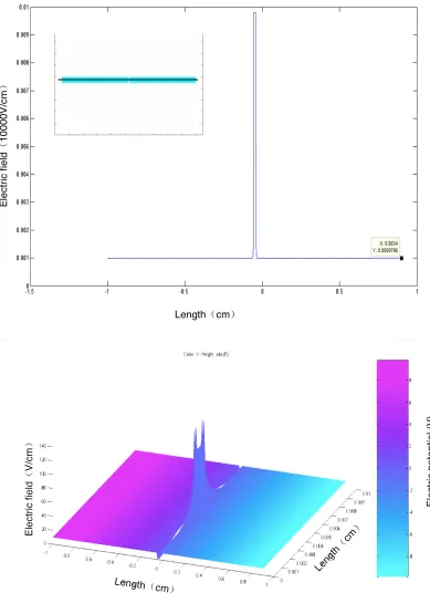
The particular shape of the microchannel design leads to a nonuniform electric field
distri-bution along the channel axis. We can estimate the local electric field strength as a function of
the applied voltage through a simple argument that considers the wide microchannel and the
narrow constriction as uniform.
From the current conservation, we have for the currents Iwide and Iconstriction
Iwide=Iconstriction (2.1)
Since I =J S =J dW, where J, S,d,W denote for current density, cross section area, depth
and width, and J =σE we have:
EwideWwide =EconstrictionWconstriction (2.2)
and thus,
Econstriction
Ewide
= Wwide
Wconstriction
= 10 (2.3)
So we expect the electric field in the constriction to be 10 times of that in the wide regions
of the microchannel. Since length of the central constriction is rather short (500µm), compared
to the total length of the whole channel (19 mm), the ohmic resistance of the whole channel
is dominated by the wide regions so the local field in the constriction can be evaluated by the
total length of the microchannel (Lengthtotal) and the voltage applied (Vtotal). Thus its value
10×Vtotal/Lengthtotal.
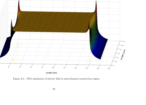
Further, considering the limited length of the constriction and the boundary conditions, a
finite element analysis (FEA) was carried out to determine what the electric field distribution
in the constriction is. It also can answer the question that what portion of the channel can
be considered to have a homogeneous field, (Figure 2.4). In this simulation, the PDE toolbox
in Matlab was used to establish the geometric configuration of one channel, and the electric
was calculated. We found that over the central 80% of the constriction the electric field was
within ±1% range of the electric field in the constriction center, (Figure 2.5). However, at the entrance to the constriction we observed significant electric field disturbances, and thus all data
Table 2.1: Measured Ionic Strength (I) of TBE Buffers [34].
buffer concentration 5× 2× 0.5× 0.1× 0.02×
I(M) 1.65×10⁻¹ 6.26×10⁻² 1.48×10⁻² 2.86×10⁻³ 5.68×10⁻⁴
2.1.2 Biological materials
We chose λ-DNA for our experiments. λ-DNA is the genomic DNA of bacteriophage λ. Each
λ-DNA molecule has 48502 base pairs. Theλ-DNA was linearized at thecossite by the vendor
(New England Biolabs). The typical Rg of a λ-DNA molecule at physiological salt strength
without any geometric constraints is ∼ 700 nm. DNA was dissolved in tris base-boric acid-EDTA (TBE) buffer solution with concentrations of 0.25×, 0.5×, 1× and 2×. 5×TBE buffer
solution consists of 54g of Tris base (CAS# 77-86-1), 27.5 g of boric acid (CAS#
10043-35-3) and 20 mL of 0.5 M EDTA (CAS# 60-00-4) [12]. Under these conditions the mechanical
properties of DNA are well-explored, and electrophoretic transport without surface adhesion
is easily established [34]. TBE buffer is typically used for DNA electrophoresis because of its
high buffer capability and low conductivity. However, the high buffer capability comes at the
expense of low buffer dissociation. Hsieh [34] also measured the ionic strength of TBE buffer in
different concentrations, shown in table 2.1.
Individual DNA molecules cannot be observed directly using a microscope due to
insuffi-cient auto-fluorescence, absorption or refractive index contrast. As a result, we used a fluorescent
dye to visualize DNA. The dye we chose was YOYO-1 (Molecular Probes/ Invitrogen), whose
chemical structure and absorption-fluorescence emission spectra are shown in Figure 2.6 and
Figure 2.7, respectively. YOYO-1 is a member of a larger family of bis-intercalating dimeric
cya-nine dyes that that provider has developed. We chose a staining ratio of 1 dye molecule every 10
base pairs. At this concentration, the dominant staining mechanism is through bis-intercalation
properties of DNA [60] [29]. The consensus finding is that DNA elongates upon dye insertion.
At 1 dye per 10 basepairs the elongation is on the order of 20%. There are some
discrepan-cies concerning the influence on the persistence length in the literature. G¨unter and co-workers
report no significant modification, while others reported a reduction of the persistence length
(for instance reduction down to 20% under severe overstaining [71]. We believe that the dye
has some influence on the molecular geometry, but will not modify the qualitative outcome of
the study and the influence of the a.c. electric field.
The dye also has a small preference for CG-rich regions, which can be detected in
exper-iments in which DNA is stretched through confinement to nanochannels or molecular
comb-ing [37]. However,λ-DNA has only a short AT-rich stretch at about 30 kbase [67], and we do
not expect that this 5 kbase region can be resolved. After sufficient thermalization [16], we thus
expect to observe the emission light of dye molecules evenly distributed in DNA molecule. We
take the fluorescence of YOYO-1 to be the mass density of DNA in our experiment.
Figure 2.6: Chemical structure of YOYO-1 iodide [62].
2.1.3 Experiment setup
We used a fluorescent microscope system together with an electron-multiplying CCD camera
(Andor, iXon+) to monitor the emission light of YOYO-1 excited by a 50 mW, 473 nm blue
laser. The schematic diagram is shown in Figure 2.8.
A fluorescent microscope is a microscope which images object by fluorescence and
Figure 2.8: Schematic diagram of fluorescent microscope [2].
reflection or transmission. The key component which differentiates fluorescent microscopes and
ordinary ones is the dichroic filter. A dichroic filter is designed that it passes a range of
wave-length of light while reflecting other ranges, (Figure 2.9). The reflection and pass spectra of the
dichroic filter set we used in our experiment is shown in Figure 2.10. 473 nm light is reflected
by the dichroic filter and illuminates the specimen, and the emitted light, ranging from 525 nm
to 562 nm, passes the filter before hitting the CCD camera.
We carefully chose a microscope objective, that allows us to achieve the resolution of the
diffraction limit while preserving a high brightness and signal to noise ratio. The resolution
of an microscope objective is limited by its numerical aperture (NA), which is the product of
refractive index of the imaging mediumnand sine of angular apertureθ. NA reflects the ability
of a given objective to gather light. We chose the maximum practical NA for water (n≈1.333), and then matched the magnification so that the resolution is not limited by pixel size of CCD.
Magnification in excess of that would lead to a lower signal to noise ratio because the brightness
Figure 2.9: The schematic of dichroic filter set [2]
be evaluated by Rayleigh’s criterion:
rlaterial =
2λ
πN A (2.4)
We used a 100×oil immersion objective with 1.3 NA. It has a 262 nm lateral resolution for
the emitted 535 nm light. The projection of the 262 nm lateral scale in image plane, e.g. CCD
surface is about 26.2µm. The CCD has 16µm×16µmpixels. Hence, the limit of resolution of the whole system is the objective, not the CCD. Under this circumstance, a higher magnification
could not really increase the resolution, only making the image spread out over more pixels.
Another characteristic of the objective which affects our experiment greatly is the depth of
field (DOF). The DOF is an axial range through which an objective can be focused without
significant loss of sharpness. It decreases with increasing NA. In general, the DOF contains
contributions from both wave optics and geometrical optics:
DOF = λn
NA2 +
ne
M NA (2.5)
fractive index of the imaging medium, objective lateral magnification and the smallest distance
that can be resolved by a detector placed in the image plane of the objective, respectively. In
our experiment, the immersion oil has a refractive index of 1.515. As a result, the DOF of this
system is around 483 nm, which is slightly smaller than theRg ofλ-DNA. We chose the channel
depth to match thisRgofλ-DNA so that the molecule is approximately free [7] [18] while being
held in the focal plane. The mismatch ofRg and DOF will lead to a small deterioration of the
minimum measurable Rg.
Steering mirror illumination system
Assume that dye molecules bind evenly to DNA, one expects the emitted light intensity is
proportional to DNA molecule mass density if the illumination field is homogeneous.
YOYO-1 dyed DNA molecules have a shorter bleach period then the total observation period
we expected. During exposure time of each frame, Brownian motion of the molecule could blur
the image taken by the CCD camera. Therefore, the incidence laser was controlled to generate
pulses instead of illuminating continuously. The pulses were synchronized with EM-CCD frame
rate as well as image recording software to increase the YOYO-1 life time without affecting
image brightness negatively or deteriorating the resolution.
An orthogonal-axis steering mirror system was thus adopted to assure the homogenous
illumination. Figure 2.11 shows the whole optical system including microscope and the steering
mirror illumination part. The two axis of mirrors are orthogonal, driven by a computer controlled
servo motor system. The two mirrors were designed different in size to minimize the load of
servo system.
The computer control system consists of a field-programmable gate array (FPGA) board
and a Labview program. The servo motor system has built-in feed back control. It converts
the input voltage signal from FPGA board into position of mirrors. A FPGA is an integrated
circuit which is programable–“field-programmable”. It contains a large number of basic “logic
blocks” such as “logic gates” or memory elements. The function of the whole integrated circuit
7841R interface card made by National Instruments that contains a Xilinx Virtex 5 FPGA.
Programs written in the Labview FPGA module are compiled and converted into hardware
description language (HDL) which could directly specify FPGA configuration. With help of the
Labview FPGA module, the FPGA communicates with the main program running on computer.
At small angle deflections of the mirrors, the optic aberrations of our optical system is
negligible. The irradiance of the incidence laser is determined by speed at which the spot moves
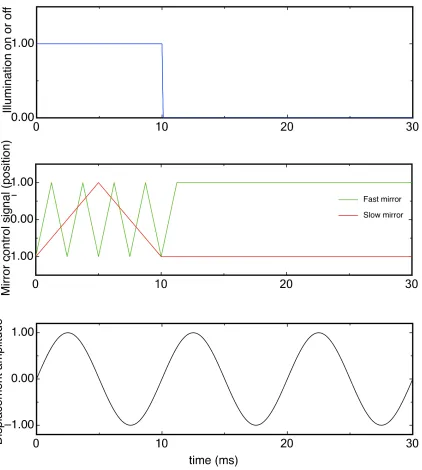
in the image plane. As a result, a constant-speed moving triangle voltage control signal was
generated for each mirror channel, (Figure 2.14).
Figure 2.14: Triangle wave steering mirror control signal.
Note that the small distortion at the peaks and valleys of the triangle signal were not due
to optical aberration but due to design and discretion nature of FPGA system–the triangle
signal is a superposition of the first three terms of the Fourier series of an ideal triangle signal,
sin(x), −19sin(3x), 251 sin(5x). The advantage of these blunt corners is that the acceleration, e.g. the second derivative of the position as a function of time, does not have infinite values,
which would push servo motor system to its power limit twice in each period. The side effect
of this feature is that it will lead to inhomogenous irradiance on edges of the illumination field.
However, by carefully tuning the amplitude of the driving signal we expanded illumination area
shown in Figure 2.13, the camera shutter (whose exposure time is about 143 ms), illumination
laser and steering mirrors are controlled and synchronized by the PC-FPGA-based system.
An extra convex lens (above the UV laser in Figure 2.11) was used to expand the area of the
incidence laser spot so that the scan lines in the image plane overlapped each other to create
seamless, homogenous illumination.
Another advantage of this system is that it eliminates interference patterns of the optical
system to a great extent. A static illumination system, in which the illumination light source
and beam path are static, can create interference patterns in the objective (specimen) plane.
This pattern would greatly affect the image and further affect the numerical measures calculated
from it. Our steering mirror illumination system, however, keeps changing the angle of incidence
light. Thus, the interference pattern caused by static components keeps changing and is averaged
out in each exposure. This characteristic also enables use of Gaussian beam.
The programable nature makes this system versatile, and enables the addition of more
functions needed for the project described in Chapter 5.
Image processing and DNA identification
For each DNA molecule, a short video (typically 30 to 45 seconds long, containing several
hundred frames) was taken. Based upon the individual frames of each video, a series of Rgs
as well as anisotropies were calculated. We diluted the DNA solution observed to a rather low
concentration so that, with the help of narrow part of the channel, only one DNA molecule was
in the view of objective at a time.
The purpose of this concentration is to reduce error inRg calculation and simplify molecule
position control. Due to the nature of the experiment (relatively low signal to noise ratio) and
the way the gyration matrix and Rg is calculated, the error of Rg is extremely sensitive to
the area and shape of the view. In other words, the accuracy of Rg calculated depends on the
chosen of calculation area–the closer to the shape of the molecule, the better. An identification
of the position of the molecule thus is needed.
the image and the signal to noise ration is rather low. Any deletion and addition of the observed
area could lead to a great relative error ofRg. The shape change of DNA molecules made this
identification even complicated.
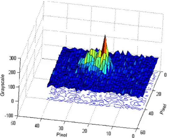
Figure 2.16: Single DNA molecule image, shown in 3-D plot (pseudo color).
We evaluated several commonly used edge detection algorithms first, including Sobel
opera-tor differential algorithm, Prewiit operaopera-tor differential algorithm, LOG and Canny operaopera-tor [85].
The reliability and accuracy were not acceptable for such a small signal-to-noise ratio images
that lack sharp edges. As a result, we adopted a hybrid method which is a mixture of
im-age grayscale threshold, morphology logic judgement, region dilation/contraction and system
characteristics analysis.
Our objects in a given series of experiment are single, connected DNA molecules. They have
several predictable characteristics:
2. The shape of the molecules changes between known patterns.
3. The background noise distribution and inhomogeneous sensitivity of CCD (if any) are
predeterminable.
Utilizing these characteristics, a matlab program was written to analyze images and
deter-mine the regions of interest. It contains the following steps:
1. Remove the bright edge band due to inhomogeneous CCD background.
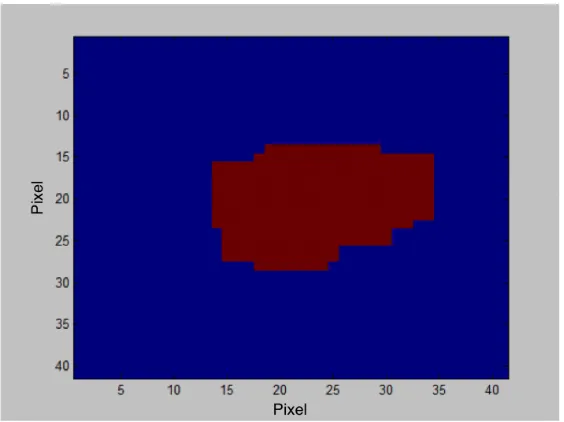
2. Determine the region which contains the target molecule, shown in Figure 2.17. Due to
the known approximate area of the molecule, we defined a thresholdT of grayscale above which
there were at most a constant number of pixels. Then convert the original grayscale image to
a binary one, e.g. a “mask of the original image”. The result is shown in Figure 2.18. This
separates the molecule and the background regions to some extent. Although the image may
contains peaks of background noise, they occupy a smaller area then the area of interest.
3. Erode and dilate the image several times. These series of operations “fuses” the possibly
separated parts near the main region of the molecule and removes most of the small, false parts
due to background noise. The result of this step updates the “mask” generated in previous steps.
4. After this, the result “mask” may still contain a plural number of regions. Some of these
regions could be fragments of other DNA molecules, others could belong to the target DNA
molecule whose connecting parts were separated in the previous steps. We will later explain why
the most frequently observed configuration with apparently disconnected domains has domains
of equal area. Noise or DNA fragments would not be of equal area as the main peak due to a
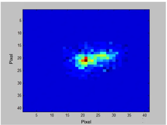
Figure 2.17: Single DNA molecule image (pseudo color).
areSi, and i= 1,2,3, ..., n. The threshold of area was chosen as:
ST =
Pn
i=1Si
n+ 1 (2.6)
All the regions whose area is below this area threshold will be dropped. And the result of this
step updates the “mask” generated in previous steps.
Manual examination showed that the result of this judgement was fairly good for our data set.
5. Let elements of the “mask” multiply all the corresponding elements in the original image,
forming a new image in which only kept region(s) of the original image presents. This eliminates
all the content from the regions other than target molecule, (Figure 2.19).
Figure 2.19: A single DNA molecule image operated by a “mask” pattern (pseudo color).
Electric field generating and feedback control system
![Figure 1.2:The bending of a small polymer segment ∆l. ⃗e(l) represents the tangential vectorat the location l [76].](https://thumb-us.123doks.com/thumbv2/123dok_us/1361953.1169022/21.612.201.394.82.247/figure-bending-polymer-segment-represents-tangential-vectorat-location.webp)
![Figure 2.7:Absorption and fluorescence emission spectra of YOYO-1 bound to DNA and filterset spectrum [62].](https://thumb-us.123doks.com/thumbv2/123dok_us/1361953.1169022/51.612.142.484.200.482/figure-absorption-uorescence-emission-spectra-yoyo-lterset-spectrum.webp)
![Figure 2.8:Schematic diagram of fluorescent microscope [2].](https://thumb-us.123doks.com/thumbv2/123dok_us/1361953.1169022/52.612.179.451.72.309/figure-schematic-diagram-of-uorescent-microscope.webp)