Extension of TSVM to Multi-Class and Hierarchical Text
Classification Problems With General Losses
S
.
Sathi ya Keer thi
(1)S
.
Sundarara jan
(2)Shirish Shevade
(3)(1) Cloud and Information Services Lab, Microsoft, Mountain View, CA 94043 (2) Microsoft Research India, Bangalore, India
(3) Computer Science and Automation, Indian Institute of Science, Bangalore, India [email protected], [email protected], [email protected]
Abstract
1 Introduction
Consider the following supervised learning problem corresponding to a general structured output prediction problem: example, in large margin and maxent models respectively we have
ξ(w,xi,yi) =maxy L(y,yi)−wT∆f(y,yi;xi)andξ(w,xi,yi) =−wTf(yi;xi) +logZ (2) where∆f(y,yi;xi) =f(yi;xi)−f(y;xi)andZ=
P
yexp(wTf(y;xi)). Text classification prob-lems involve a rich and large feature space (e.g., bag-of-words features) and so linear classifiers work very well (Joachims, 1999). We particularly focus on multi-class and hierarchical classifi-cation problems (and hence our use of scalar notation fory). In multi-class problemsyruns over the classes and,wandf(y;xi)have one component for each class, with the component corresponding toyturned on. More generally, in hierarchical classification problems,yruns over the set of leaf nodes of the hierarchy and,wandf(y;xi)consist of one component for each node of the hierarchy, with the node components in the path to leaf nodeyturned on. λ >0 is a regularization parameter. A good default value forλcan be chosen depending on the loss function used.1The superscriptsdenotes ‘supervised’; we will use superscriptuto denote elements corresponding to unlabeled examples.
In semi-supervised learning we use a set of unlabeled examples, {xu
i}ni=1 and include the determination of the labels of these examples as part of the training process:
min parameter for the unlabeled part. A good default value isCu=1; we use this value in all our experiments. (3) consists of constraints on the label counts that come from domain knowledge. (In practice, one specifiesφ(y), the fraction of examples in classy; then the values in{φ(y)n}
are rounded to integers{n(y)}in a suitable way so thatPyn(y) =n.2) Such constraints are crucial for the effective solution of the semi-supervised learning problem; without them the semi-supervised solution tends to move towards assigning the majority class label to most unlabeled examples. In more general structured prediction problems (3) may include other domain constraints (Chang et al., 2007). In this paper we will use just the label constraints in (3).
Inspired by the effectiveness of the TSVM model of Joachims (1999), there have been a number of works on the solution of (3) for binary classification with large margin losses. These methods fall into one of two types: (a) combinatorial optimization; and (b) continuous optimization.
1In the experiments of this paper, for multi-class and hierarchical classification with large margin loss, we use
λ=10.
2We will assume that quite precise values are given for{n(y)}. The effect of noise in these values on the
See (Chapelle et al., 2008, 2006) for a detailed coverage of various specific methods falling into these two types. In combinatorial optimization the label setyuis determined together with w. It is usual to use a sequence of alternating optimization steps (fixyuand solve forw, and then fixwand solve foryu) to obtain the solution. An important advantage of doing this is that each of the sub-optimization problems can be solved using simple and/or standard solvers. In continuous optimizationyuis eliminated and the resulting (non-convex) optimization problem is solved forwby minimizing
Fs(w) +Cu n
n X
i=1 ρ(w,xu
i) (4)
whereρ(w,xu
i) =minyuξ(w,xiu,yiu). The loss functionξas well asρare usually smoothed so that the objective function is differentiable and gradient-based optimization techniques can be employed. Further, the constraints in (3) involvingyuare replaced by smooth constraints onw expressing balance of the mean outputs of each label over the labeled and unlabeled sets. Zien et al. (2007) extended the continuous optimization approach to (4) for multi-class and structured output problems. But their experiments only showed limited improvement over supervised learning. The combinatorial optimization approach, on the other hand, has not been carefully explored beyond binary classification. Methods based on semi-definite program-ming (Xu et al., 2006; De Bie and Cristianini, 2004) are impractical, even for medium size problems. One-versus-rest and one-versus-one ideas have been tried, but it is unclear if they work well: Zien et al. (2007) and Zubiaga et al. (2009) report failure while Bruzzone et al. (2006) use a heuristic implementation and report success in one application domain. Unlike these methods which have binary TSVM as the basis, we take up an implementation of the approach for the direct multi-class and hierarchical classification formulation in (3). The special structure in constraints allows theyudetermination step to reduce to a degenerate transporta-tion linear programming problem. So the well-known transportatransporta-tion simplex method can be used to obtainyu. We show that even this method is not efficient enough. As an alternative we suggest an effective and much more efficient heuristic label switching algorithm. For binary classification problems this algorithm is an improved version of the multiple switching algorithm developed by Sindhwani and Keerthi (2006) for TSVM. Experiments on a number of multi-class and hierarchical classification datasets show that, like the TSVM method of binary classification, our method yields a strong lift in performance over supervised learning, especially when the number of labeled examples is not sufficiently large. Although we demonstrate our method using hinge loss, the applicability of our approach to general loss functions (e.g., maxent loss) is a key advantage. The reader is referred to the longer version of this paper (Keerthi et al., 2012) for details on specialization to maxent losses ((Gärtner et al., 2005), (Graca et al., 2007), (Ganchev et al., 2009) and (Mann and McCallum, 2010)) and more experimental results.
2 Semi-Supervised Learning Algorithm
The semi-supervised learning algorithm for multi-class and hierarchical classification problems follows the spirit of the TSVM algorithm (Joachims, 1999). Algorithm 1 gives the steps. It consists of an initialization part (steps 1-9) that sets starting values forwandyu, followed by an iterative part (steps 10-15) wherewandyuare refined by semi-supervised learning. Using exactly the same arguments as those in (Joachims, 1999; Sindhwani and Keerthi, 2006) it can be proved that Algorithm 1 is convergent.
to predictyu. However such ayuusually violates the constraints in (3). To choose ayuthat satisfies (3), we do a greedy modification of the predictedyu. Steps 3-9 of Algorithm 1 give the details.
The iterative part of the algorithm consists of an outer loop and an inner loop. In the outer loop (steps 10-15) the regularization parameterCuis varied from a small value to the final value of 1 in annealing steps. This is done to avoid drastic switchings of the labels inyu, which helps the algorithm reach a better minimum of (3) and hence achieve better performance. For example, on ten runs of the multi-class dataset,20NG(see Table 1) with 100 labeled examples and 10, 000 unlabeled examples, the average macro F values on test data achieved by supervised learning, Algorithm 1 without annealing and Algorithm 1 with annealing are, respectively, 0.4577, 0.5377 and 0.6253. Similar performance differences are seen on other datasets too. The inner loop (steps 11-14) does alternating optimization ofwandyufor a givenCu. In steps 12 and 13 we use the most recentwandyu as the starting points for the respective sub-optimization problems. Because of this, the overall algorithm remains very efficient in spite of the many annealing steps involvingCu. Typically, the overall cost of the algorithm is only about 3-5 times that of solving a supervised learning problem involving(n+l)examples. For step 12 one can employ any standard algorithm suited to the chosen loss function. In the rest of the section we will focus on step 13.
Algorithm 1Semi-Supervised Learning Algorithm 1: Solve the supervised learning problem, (1) and getw.
2: Set initial labels for unlabeled examples,yuusing steps 3-9 below. 3: SetY={y}, the set of all classes,Ay=; ∀y, andI={1, . . . ,n}. 4: repeat
5: Si=maxy∈YwTf(y;xui)andyi=arg maxy∈YwTf(y;xui)∀i∈I. 6: SortIby decreasing order ofSi.
7: By order allocateitoAyiwhile not exceeding sizes specified byn(yi).
8: Remove all allocatedifromIand remove all saturatedy(i.e.,|Ay|=n(y)) fromY. 9: untilY=;
10: forCu={10−4, 3×10⁻⁴, 10−3, 3×10⁻³, . . . , 1}(in that order)do
11: repeat
12: Solve (3) forwwithyufixed (i.e., without constraints). 13: Solve (3) foryuwithwfixed.
14: untilstep 13 does not alteryu 15: end for
2.1 Linear programming formulation
Let us now consider optimizingyuwith fixedw. Let us represent eachyu
i in a 1-of-m represen-tation by defining boolean variableszi yand requiring that, for eachi, exactly onezi ytakes the value 1. This can be done by using the constraintPyzi y=1 for alli. The label constraints becomePizi y=n(y)for ally. Letci y=ξ(w,xui,y). With these definitions the optimization problem of step 13 becomes (irrespective of the type of loss function used) the integer linear programming problem,
min X i,y
ci yzi y s.t. X
y
zi y=1 ∀i, X
i
This is a special case of the well known Transportation problem (Hadley, 1963) in which the constraint matrix satisfies unimodularity conditions; hence, the solution of the integer linear programming problem (5) is same as the solution of the linear programming (LP) problem (i.e., with the integer constraints left out), i.e., the integer constraints hold automatically at LP optimality. Previous works (Joachims, 1999; Sindhwani and Keerthi, 2006) do not make this neat connection to linear programming. The constraintsPyzi y=1∀iallow exactlynnon-zero elements in{zi y}i y; thus there is degeneracy of orderm, i.e., there are(n+m)constraints but onlynnon-zero solution elements.
2.2 Transportation simplex method
The transportation simplex method (a.k.a., stepping stone method) (Hadley, 1963) is a standard and generally efficient way of solving LPs such as (5). However, it is not efficient enough for typical large scale learning situations in whichn, the number of unlabeled examples is large and m, the number of classes, is small. Let us see why. Each iteration of this method starts with a basis set ofn+m−1 basis elements. Then it computes reduced costs for all remaining elements. This step requiresO(nm)effort. If all reduced costs are non-negative then it implies that the current solution is optimal. If this condition does not hold, elements which have negative reduced costs are potential elements for entering the basis.3 One non-basis element with a negative reduced cost (say, the element with the most negative reduced cost) is chosen. The algorithm now moves the solution to a new basis in which an element of the previous basis is replaced by the newly entering element. This operation corresponds to moving a chosen set of examples between classes in a loop so that the label constraints are not violated. The number of such iterations is observed to beO(nm)and so, the algorithm requiresO(n2m2)time. Sincen can be large in semi-supervised learning, the transportation simplex algorithm is not sufficiently efficient. The main cause of inefficiency is that the step (one basis element changed) is too small for the amount of work put in (computing all reduced costs)!
2.3 Switching algorithm
We now propose an efficient heuristicswitching algorithmfor solving (5) that is suited to the case wherenis large butmis small. The main idea is to use only pairwise switching of labels between classes in order to improve the objective function. (Note that switching makes sure that the label constraints are not violated.) This algorithm is sub-optimal form≥3, but still quite powerful because of two reasons: (a) the solution obtained by the algorithm is usually close to the true optimal solution; and (b) reaching optimality precisely is not crucial for the alternating optimization approach (steps 12 and 13 of Algorithm 1) to be effective.
Let us now give the details of the switching algorithm. Suppose, in the current solution, example iis in classy. Let us say we move this example to class ¯y. The change in objective function due to the move is given byδc(i,y, ¯y) =ci¯y−ci y. Suppose we have another example ¯iwhich is currently in class ¯y and we switchiand ¯i, i.e., moveito class ¯yand move ¯ito classy. The resulting change in objective function is given byρ(i,y, ¯i, ¯y) =δc(i,y, ¯y) +δc(¯i, ¯y,y). The more negativeρ(i,y, ¯i, ¯y)is, the better will be the objective function reduction due to the
switching ofiand ¯i. The algorithm looks greedily for finding as many good switches as possible
3Presence of negative reduced costs may not mean that the current solution is non-optimal. This is due to degeneracy.
Algorithm 2Switching Algorithm to solve(5) 1: repeat
2: foreach class pair(y, ¯y)do
3: Computeδc(i,y, ¯y)for alliin classyand sort the elements in increasing order ofδc values.
4: Computeδc(¯i, ¯y,y)for all ¯iin class ¯yand sort the elements in increasing order ofδc values.
5: Align these two lists (so that the best pair is at the top) to form a switch list of 5-tuples,
{(i,y, ¯i, ¯y,ρ(i,y, ¯i, ¯y)}.
6: Remove any 5-tuple withρ(i,y, ¯i, ¯y)≥0. 7: end for
8: Merge all the switch lists into one and sort the 5-tuples by increasing order ofρvalues. 9: whileswitch list is non-emptydo
10: Pick the top 5-tuple from the switch list; let’s say it is(i,y, ¯i, ¯y,ρ(i,y, ¯i, ¯y)). Moveito class ¯yand move ¯ito classy.
11: From the remaining switch list remove all 5-tuples involving eitherior ¯i. 12: end while
13: untilthe merged switch list from step 8 is empty
at a time. Algorithm 2 gives the details. Steps 2-12 consist of one major greedy iteration and has costO(nm2). Steps 2-7 consist of the background work needed to do the greedy switching of several pairs of examples in steps 9-12. Step 11 is included because, wheniand ¯iare switched, data related to any 5-tuple in the remaining switch list that involves eitherior ¯iis messed up. Removing such elements from the remaining switched list allows the algorithm to continue finding more pairs to apply switching without a need for repeating steps 2-7. It is this multiple switching idea that gives the needed efficiency lift over the transportation simplex algorithm. The algorithm is convergent due to the following reasons: the algorithm only performs switch-ings which reduce the objective function; thus, once a pair of examples is switched, that pair will not be switched again; and, the number of possible switchings is finite. A typical run of Algorithm 2 requires about 3 loops through steps 2-12. Since this algorithm only allows pairwise switching of examples, it cannot assure that the class assignments resulting from it will be optimal for (5) ifm≥3. However, in practice the objective function achieved by the algorithm is very close to the true optimal value; also, as pointed out earlier, reaching true optimality turns out to be not crucial for good performance of the semi-supervised algorithm. We compared the speed performance of transportation simplex and switching algorithms on real-world datasets such asOhscaland found that the switching algorithm is faster by two orders of magnitude. Note that ifmis large then steps 2-7 of Algorithm 2 can become expensive. We have applied the switching algorithm to datasets that havem≤105, but haven’t observed any inefficiency. Ifmhappens to be much larger then steps 2-7 can be modified to work with a suitably chosen subset of class pairs instead of all possible pairs.
3 Experiments with large margin loss
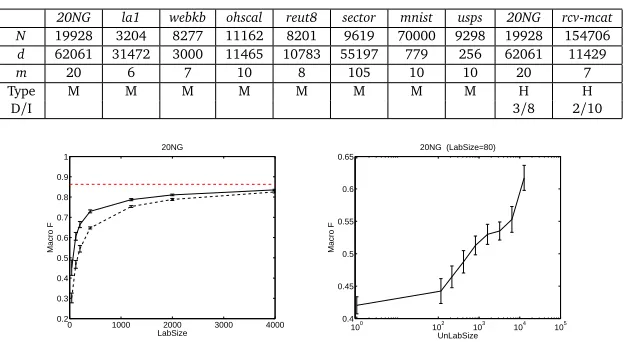
Table 1: Properties of datasets.N: number of examples,d: number of features,m: number of classes, Type: M=Multi-Class; H=Hierarchical, with D=Depth and I=# Internal Nodes
20NG la1 webkb ohscal reut8 sector mnist usps 20NG rcv-mcat
N 19928 3204 8277 11162 8201 9619 70000 9298 19928 154706
d 62061 31472 3000 11465 10783 55197 779 256 62061 11429
m 20 6 7 10 8 105 10 10 20 7
Figure 1: Hierarchical classification dataset - Variation of performance (Macro F):Left- as a function of the number of labeled examples (LabSize). Dashed black line corresponds to supervised learning; Continuous black line corresponds to the semi-supervised method; Dashed horizontal red line corresponds to the supervised classifier built usingLandUwith their labels known. Right- as a function of the number of unlabeled examples (UnLabSize), with the number of labeled examples fixed at 80.
used. Due to lack of space, performance results are given only for some datasets. The reader is referred to the longer version of this paper (Keerthi et al., 2012) for details on other data sets. Properties of these datasets (Lang, 1995; Forman, 2003; McCallum and Nigam, 1998; Lewis et al., 2006; LeCun, 2011; Tibshirani, 2011) are given in Table 1. Most of these datasets are standard text classification benchmarks. We include two image datasets,mnistanduspsto point out that our methods are useful in other application domains too.rcv-mcatis a subset of rcv1 (Lewis et al., 2006) corresponding to the sub-tree belonging to the high level category MCAT with seven leaf nodes consisting of the categories, EQUITY, BOND, FOREX, COMMODITY, SOFT, METALand ENERGY. In one run of each dataset, 50% of the examples were randomly chosen to form the unlabeled set,U; 20% of the examples were put aside in a setLto form labeled data; the remaining data formed the test set. Ten such runs were done to compute the mean and standard deviation of (test) performance. Performance was measured in terms of Macro F (mean of the F values associated with various classes).
0 200 400 600 800 1000
0 500 1000 1500 2000 2500 0.35
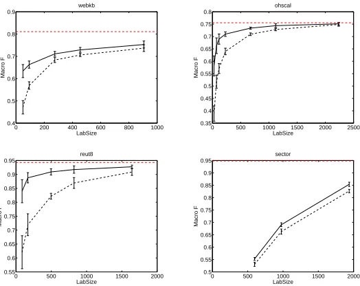
Figure 2: Multi-class datasets: Variation of performance (Macro F) as a function of the number of labeled examples (LabSize). Dashed black line corresponds to supervised learning; Continuous black line corresponds to the semi-supervised method; Dashed horizontal red line corresponds to the supervised classifier built usingLandUwith their labels known.
data is sparse (lower side of the learning curve). The variation of performance as a function of the number of labeled examples is shown in Figure 1 (Left). The same holds in other datasets too. The results for four multi-class datasets are given in Figure 2. Clearly, semi-supervised learning is very useful and yields good improvement over supervised learning especially when labeled data is sparse. The degree of improvement is sharp in some datasets (e.g.,reut8) and mild in some datasets (e.g.,sector). While the semi-supervised method is successful in linear classifier settings such as in text classification and natural language processing, we want to caution, like (Chapelle et al., 2008), that it may not work well on datasets originating from nonlinear manifold structure.
4 Conclusion
References
Bruzzone, L., Chi, M., and Marconcini, M. (2006). A novel transductive SVM for semisupervised classification of remote-sensing images. volume 44, pages 3363–3373.
Chang, M. W., Ratinov, L., and Roth, D. (2007). Guiding semi-supervision with constraint-driven learning. InACL.
Chapelle, O., Chi, M., and Zien, A. (2006). A continuation method for semi-supervised SVMs. InICML.
Chapelle, O., Sindhwani, V., and Keerthi, S. S. (2008). Optimization techniques for semi-supervised support vector machines. InJMLR, volume 9, pages 203–233.
De Bie, T. and Cristianini, N. (2004). Convex methods for transduction. InNIPS.
Forman, G. (2003). An extensive empirical study of feature selection metrics for text classifica-tion. InJMLR, volume 3, pages 1289–1305.
Ganchev, K., Graca, J., Gillenwater, J., and Taskar, B. (2009). Posterior regularization for structured latent variable models. Technical report, Dept. of Computer & Information Science, University of Pennsylvania.
Gärtner, T., Le, Q. V., Burton, S., Smola, A. J., and Vishwanathan, S. V. N. (2005). Large-scale multiclass transduction. InNIPS.
Graca, J., Ganchev, K., and Taskar, B. (2007). Expectation maximization and posterior constraints. InNIPS.
Hadley, G. (1963).Linear Programming. Addison-Wesley, 2nd edition.
Joachims, T. (1999). Transductive inference for text classification using support vector machines. InICML.
Keerthi, S. S., Sundararajan, S., and Shevade, S. (2012). Extension of TSVM to multi-class and hierarchical text classification problems with general losses.http://arxiv.org/abs/ 1211.0210.
Lang, K. (1995). Newsweeder: Learning to filter netnews. InICML. LeCun, Y. (2011). The MNIST database of handwritten digits.
Lewis, D., Yang, Y., Rose, T., and Li, F. (2006). Rcv1: A new benchmark collection for text categorization research. InJMLR, volume 5, pages 361–397.
Mann, G. S. and McCallum, A. (2010). Generalized expectation criteria for semi-supervised learning with weakly labeled data. InJMLR, volume 11, pages 955–984.
McCallum, A. and Nigam, K. (1998). A comparison of event models for naive Bayes text classification. InAAAI Workshop on Learning for Text Categorization.
Xu, L., Wilkinson, D., Southey, F., and Schuurmans, D. (2006). Discriminative unsupervised learning of structured predictors. InICML.
Zien, A., Brefeld, U., and Scheffer, T. (2007). Transductive support vector machines for structured variables. InICML.