Improving Graph based Dependency Parsing with Decision History

(1)

Improving Graph-based Dependency Parsing with Decision History

Wenliang Chen†_{, Jun’ichi Kazama}†_{, Yoshimasa Tsuruoka}†‡ _{and Kentaro Torisawa}† †_{Language Infrastructure Group, MASTAR Project, NICT}

{chenwl, kazama, torisawa_}@nict.go.jp ‡_{School of Information Science, JAIST}

[email protected]

Abstract

This paper proposes an approach to im-prove graph-based dependency parsing by using decision history. We introduce a mechanism that considers short dependen-cies computed in the earlier stages of pars-ing to improve the accuracy of long de-pendencies in the later stages. This re-lies on the fact that short dependencies are generally more accurate than long depen-dencies in graph-based models and may be used as features to help parse long de-pendencies. The mechanism can easily be implemented by modifying a graph-based parsing model and introducing a set of new features. The experimental results show that our system achieves state-of-the-art accuracy on the standard PTB test set for English and the standard Penn Chi-nese Treebank (CTB) test set for ChiChi-nese.

1 Introduction

Dependency parsing is an approach to syntactic analysis inspired by dependency grammar. In re-cent years, interest in this approach has surged due to its usefulness in such applications as machine translation (Nakazawa et al., 2006), information extraction (Culotta and Sorensen, 2004).

Graph-based parsing models (McDonald and Pereira, 2006; Carreras, 2007) have achieved state-of-the-art accuracy for a wide range of lan-guages as shown in recent CoNLL shared tasks (Buchholz et al., 2006; Nivre et al., 2007). How-ever, to make parsing tractable, these models are forced to restrict features over a very limited his-tory of parsing decisions (McDonald and Pereira, 2006; McDonald and Nivre, 2007). Previous work showed that rich features over a wide range of decision history can lead to significant

im-provements in accuracy for transition-based mod-els (Yamada and Matsumoto, 2003a; Nivre et al., 2004).

In this paper, we propose an approach to im-prove graph-based dependency parsing by using decision history. Here, we make an assumption: the dependency relations between words with a short distance are more reliable than ones between words with a long distance. This is supported by the fact that the accuracy of short dependencies is in general greater than that of long dependen-cies as reported in McDonald and Nivre (2007) for graph-based models. Our idea is to use deci-sion history, which is made in previous scans in a bottom-up procedure, to help parse other words in later scans. In the bottom-up procedure, short de-pendencies are parsed earlier than long dependen-cies. Thus, we introduce a mechanism in which we treat short dependencies built earlier as deci-sion history to help parse long dependencies in later stages. It can easily be implemented by mod-ifying a graph-based parsing model and designing a set of features for the decision history.

To demonstrate the effectiveness of the pro-posed approach, we present experimental results on English and Chinese data. The results indi-cate that the approach greatly improves the accu-racy and that richer history-based features indeed make large contributions. The experimental re-sults show that our system achieves state-of-the-art accuracy on the data.

2 Motivation

In this section, we present an example to show the idea of using decision history in a dependency parsing procedure.

(2)

w3:买(bought) to w5:书(books) mean that w3 is

the head and w5 is the dependent. In Chinese,

the relationship between clauses is often not made explicit and two clauses may simply be put to-gether with only a comma (Li and Thompson, 1997). This makes it hard to parse Chinese sen-tences with several clauses.

ROOT

৫ᒤ ᡁ Ҡ Ҷ Җ ˈ Ӻᒤ Ԇ ҏ Ҡ Ҷ Җ

(last year) (I) (bought) (NULL) (books) (,) (this year) (he) (also) (bought) (NULL) (books) w1 w2 w3 w4 w5 w6 w7 w8 w9 w10 w11 w12

(Last year I bought some books and this year he also bought some books.)

Figure 1: Example A

ROOT

৫ᒤ ᡁ Ҡ Ҷ Җ ˈ Ӻᒤ ҏ Ҡ Ҷ Җ

(last year) (I) (bought) (NULL) (books) (,) (this year) (also) (bought) (NULL) (books) w1 w2 w3 w4 w5 w6 w7 w8 w9 w10 w11 (Last year I bought some books and this year too)

(Last year I bought some books and this year too)

Figure 2: Example B

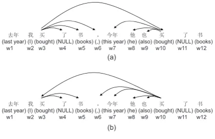
If we employ a graph-based parsing model, such as the model of (McDonald and Pereira, 2006; Carreras, 2007), it is difficult to assign the

relations betweenw3 andw10 in Example A and

betweenw3 andw9in Example B. For simplicity,

we usew_iAto refer towiof Example A andwBi to

refer towiof Example B in what follows.

The key point is whether the second clauses are independent in the sentences. The two sentences are similar except that the second clause of ple A is an independent clause but that of

Exam-ple B is not. wA

10is the root of the second clause

of Example A with subjectw₈A, while w₉B is the

root of the second clause of Example B, but the clause does not have a subject. These mean that

the correct decisions are to assignwA₁₀as the head

ofw₃AandwB₃ as the head ofwB₉, as shown by the

dash-dot-lines in Figures 1 and 2.

However, the model can use very limited infor-mation. Figures 3-(a) and 4-(a) show the right dependency relation cases and Figures 3-(b) and 4-(b) show the left direction cases. For the right direction case of Example A, the model has the

information about wA₃’s rightmost child wA₅ and

wA

10’s leftmost childw6AinsidewA3 andw10A, but it

does not have information about the other children

৫ᒤ ᡁ Ҡ Ҷ Җ ˈ Ӻᒤ Ԇ ҏ Ҡ Ҷ Җ (last year) (I) (bought) (NULL) (books) (,) (this year) (he) (also) (bought) (NULL) (books)

w1 w2 w3 w4 w5 w6 w7 w8 w9 w10 w11 w12

(a)

(b)

( y ) ( ) ( g ) ( ) ( ) (,) ( y ) ( ) ( ) ( g ) ( ) ( )

w1 w2 w3 w4 w5 w6 w7 w8 w9 w10 w11 w12

Figure 3: Example A: two directions

(last year) (I) (bought) (NULL) (books) (,) (this year) (also) (bought) (NULL) (books) w1 w2 w3 w4 w5 w6 w7 w8 w9 w10 w11

(a)

(last year) (I) (bought) (NULL) (books) ( ) (this year) (also) (bought) (NULL) (books)

(b)

(last year) (I) (bought) (NULL) (books) (,) (this year) (also) (bought) (NULL) (books) w1 w2 w3 w4 w5 w6 w7 w8 w9 w10 w11

Figure 4: Example B: two directions

(such aswA

8) ofw3AandwA10, which may be useful

for judging the relation betweenwA₃ andw₁₀A. The

parsing model can not find the difference between the syntactic structures of two sentences for pairs (wA₃,wA₁₀) and (wB₃,w₉B). If we can provide the

in-formation about the other children ofwA₃ andwA₁₀

to the model, it becomes easier to find the correct

direction betweenw₃AandwA₁₀.

Next, we show how to use decision history to

help parsew₃AandwA₁₀of Example A.

In a bottom up procedure, the relations between

the words inside [wA₃, wA₁₀] are built as follows

before the decision forwA₃ andw₁₀A. In the first

round, we build relations for neighboring words

(word distance1_{=1), such as the relations between}

w₃Aandw₄Aand betweenw₄Aandw₅A. In the

sec-ond round, we build relations for words of dis-tance 2, and then for longer disdis-tance words until all the possible relations between the inside words are built. Figure 5 shows all the possible relations

inside [w₃A, w₁₀A] that we can build. To simplify,

we use undirected links to refer to both directions

1_{Word distance between}_w

(3)

of dependency relations between words in the fig-ure.

w1 w2 w3 w4 w5 w6 w7 w8 w9 w10 w11 w12

Figure 5: Example A: first step

Then given those inside relations, we choose the inside structure with the highest score for each

direction of the dependency relation betweenwA₃

and wA

10. Figure 6 shows the chosen structures.

Note that the chosen structures for two directions could either be identical or different. In Figure 6-(a) and -(b), they are different.

w1 w2 w3 w4 w5 w6 w7 w8 w9 w10 w11 w12

(a)

w1 w2 w3 w4 w5 w6 w7 w8 w9 w10 w11 w12

(b)

w1 w2 w3 w4 w5 w6 w7 w8 w9 w10 w11 w12 (b)

Figure 6: Example A: second step

Finally, we use the chosen structures as

deci-sion history to help parse wA₃ andwA₁₀. For

ex-ample, the fact thatwA₈ is a dependent of wA₁₀is

a clue that suggests that the second clause may be

independent. This results inw₁₀A being the head of

wA₃.

This simple example shows how to use the cision history to help parse the long distance de-pendencies.

3 Background: graph-based parsing models

Before we describe our method, we briefly intro-duce the graph-based parsing models. We denote

input sentencewbyw= (w0, w1, ..., wn), where

w0=ROOT is an artificial root token inserted at

the beginning of the sentence and does not depend

on any other token inwandwirefers to a word.

We employ the second-order projective graph-based parsing model of Carreras (2007), which is an extension of the projective parsing algorithm of Eisner (1996).

The parsing algorithms used in Carreras (2007) independently find the left and right dependents of a word and then combine them later in a bottom-up style based on Eisner (1996). A subtree that

spans the words in [s, t] (and roots at s or t) is

represented by chart item[s, t, right/lef t, C/I],

where right (left) indicates that the root of the

sub-tree iss(t) andCmeans that the item iscomplete

while I means that the item is incomplete

(Mc-Donald, 2006). Here, complete itemin the right

(left) direction means that the words other thans

(t) cannot have dependents outside [s, t]and

in-complete itemin the right (left) direction, on the

other hand, means thatt(s) may have dependents

outside[s, t]. In addition,t(s) is the direct

depen-dent ofs(t) in the incomplete item with the right

(left) direction.

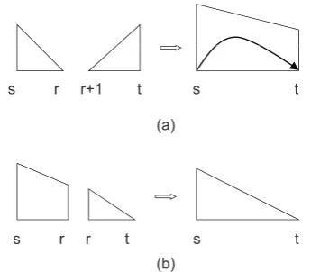
Larger chart items are created from pairs of smaller chart items by the bottom-up procedure. Figure 7 illustrates the cubic parsing actions of the Eisner’s parsing algorithm (Eisner, 1996) in the

right direction, wheres,r, andtrefer to the start

and end indices of the chart items. In Figure 7-(a), all the items on the left side are complete and

represented by triangles, where the triangle of [s,

r] is complete item[s, r,→, C]and the triangle of

[r+ 1,t] is complete item[r+ 1, t,←, C]. Then

the algorithm creates incomplete item[s, t,_→, I]

(trapezoid on the right side of Figure 7-(a)) by combining the chart items on the left side. This

action builds the dependency fromstot. In

Fig-ure 7-(b), the item of [s, r] is incomplete and

the item of [r, t] is complete. Then the

algo-rithm creates complete item[s, t,_→, C]. For the

left direction case, the actions are similar. Note that only the actions of creating the incomplete chart items build new dependency relations be-tween words, while the ones of creating the com-plete items merge the existing structures without building new relations.

(4)

to dependency relations between words of dis-tance 2, and so on by the parsing actions. For words of distance 2 and greater, it considers ev-ery possible partition of the structures into two parts and chooses the one with the highest score for each direction. The score is the sum of the fea-ture weights of the chart items. The feafea-tures are designed over edges of dependency trees and the weights are given by model parameters (McDon-ald and Pereira, 2006; Carreras, 2007). We store the obtained chart items in a table. The chart item includes the information on the optimal splitting point of itself. Thus, by looking up the table, we can obtain the best tree structure (with the highest score) of any chart item.

s r r+1 t s t

(a)

s r r t s t

(b)

Figure 7: Cubic parsing actions of Eisner (1996)

4 Parsing with decision history

As mentioned above, the actions for creating the incomplete items build the relations between words. In this study, we only consider using his-tory information when creating incomplete items.

4.1 Decision history

Suppose we are going to compute the scores of

the relations between ws andwt. There are two

possible directions for them.

By using the bottom-up style algorithm, the scores of the structures between words with

dis-tance<_|s₋t_|are computed in previous scans and

the structures are stored in the table. We divide the decision history into two types: history-inside and history-outside. The history-inside type is the

decision history made inside [s,t] and the history-outside type is the history made history-outside [s,t].

4.1.1 History-inside

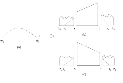
We obtain the structure with the highest score

for each direction of the dependency betweenws

andwt. Figure 8-(b) shows the best solution (with

the highest score) of the left direction, where the

structure is split into two parts,[s, r1,→, C]and

[r1+ 1, t,←, C]. Figure 8-(c) shows the best

so-lution of the right case, where the structure is split into two parts,[s, r2,→, C]and[r2+ 1, t,←, C].

s r1 r1+1 t

ws … wt

(b)

(a)

s r r +1 t

s r2 r2+1 t

(c)

Figure 8: History-inside

By looking up the table, we have a subtree that

roots atws on the right side ofws and a subtree

that roots atwton the left side ofwt. We use these

structures as the information on history-inside.

4.1.2 History-outside

For history-outside, we try to obtain the

sub-tree that roots at ws on the left side of ws and

the one that roots at wt on the right side of wt.

However, compared to history-inside, obtaining history-outside is more complicated because we do not know the boundaries and the proper struc-tures of the subtrees. Here, we use an simple heuristic method to find a subtree whose root is

atwson the left side ofwsand one whose root is

atwton the right side ofwt.

We introduce two assumptions: 1) The

struc-ture within a sub-sentence2_{is more reliable than}

the one that goes across from sub-sentences. 2) More context (more words) can result in a better solution for determining subtree structures.

2_{To simplify, we split one sentence into sub-sentences}

(5)

Algorithm 1 Searching for history-outside boundaries

1: Input:w, s, t 2: fork=s₋1to1do

3: if(isPunct(wk)) break; 4: if(s₋k >=t₋s₋1) break 5: end for

6: bs=k

7: fork=t+ 1to|w_|do 8: if(isPunct(wk)) break; 9: if(k−t >=t−s−1) break 10: end for

11: bt=k 12: Output:bs, bt

Under these two assumptions, Algorithm 1 shows the procedure for searching for

history-outside boundaries, wherebs is the boundary for

for the descendants on the left side of ws , bt

is the boundary for searching the descendants on

the right side of wt, and isPunct is the function

that checks if the word is a punctuation mark. bs

should be in the same sub-sentence with s and

|s−bs|should be less than|t−s|.btshould be in

the same sub-sentence withtand|bt−t|should

be less than|t₋s_|.

Next we try to find the subtree structures. First, we collect the part-of-speech (POS) tags of the heads of all the POS tags in training data and remove the tags that occur fewer than 10 times. Then, we determine the directions of the relations

by looking up the collected list. Forbsands, we

check if the POS tag ofws could be the head tag

of the POS tag of wbs by looking up the list. If

so, the direction dis_←. Otherwise, we check if

the POS tag of wbs could be the head tag of the

POS tag of ws. If so,d is →, else dis ←.

Fi-nally, we obtain the subtree ofwsfrom chart item

[bs, s, d, I]. Similarly, we obtain the subtree ofwt.

Figure 9 shows the history-outside information for

wsandwt, where the relation betweenwbsandws

and the relation between wbt andwt will be

de-termined by the above method. We have subtree [rs, s, lef t, C]that roots atws on the left side of

wsand subtree[t, rt, right, C]that roots atwton

the right side ofwtin Figure 9-(b) and (c).

4.2 Parsing algorithm

Then, we explain how to use these decision

his-tory in the parsing algorithm. We useLst to

rep-bs rs s t rt bt

(b)

ws … wt

(b)

(a)

b r s t r b

(c)

bsrs s t rt bt

Figure 9: History-outside

resent the scores of basic features for the left

di-rection andRstfor the right case. Then we design

history-based features (described in Section 4.3) based on the history-inside and history-outside in-formation, as mentioned above. Finally, we up-date the scores with the ones of the history-based features by the following equations:

L+_st =Lst+Ldfst (1)

R+_st=Rst+Rdfst (2)

whereL+_standR+_strefer to the updated scores,Ldf_st

and Rdf_st refer to the scores of the history-based

features.

Algorithm 2Parsing algorithm

1: Initialization:V[s, s, dir, I/C] = 0.0∀s, dir 2: fork= 1tondo

3: fors= 0ton₋kdo

4: t=s+k

5: % Create incomplete items

6: Lst=V[s, t,←, I]=maxs≤r<tV I(r); 7: Rst=V[s, t,→, I]=maxs≤r<tV I(r); 8: CalculateLdfstandRdfst;

9: % Update the scores of incomplete chart items 10: V[s, t,←, I]=L+st=Lst+Ldfst

11: V[s, t,_→, I]=R+

st=Rst+Rdfst 12: % Create complete items

13: V[s, t,_←, C]=maxs≤r<tV C(r); 14: V[s, t,_→, C]=maxs<r≤tV C(r);

15: end for

16: end for

Algorithm 2 is the parsing algorithm with

the history-based features, whereV[s, t, dir, I/C]

refers to the score of chart item [s, t, dir, I/C],

V I(r) is a function to search for the optimal

(6)

splitting pointrand return the score of the

struc-ture, andV C(r)is a function to search for the

op-timal grandchild node for the complete items (line 13 and 14). Compared with the parsing algorithms of Carreras (2007), Algorithm 2 uses history in-formation by adding line 8, 10, and 11.

In Algorithm 2, it first creates chart items with distance 1, then goes on to chart items with dis-tance 2, and so on. In each round, it searches for the structures with the highest scores for incom-plete items shown at line 6 and 7 of Algorithm 2. Then we update the scores with the history-based features by Equation 1 and Equation 2 at line 10 and 11 of Algorithm 2. However, note that we can not guarantee to find the candidate with the high-est score with Algorithm 2 because new features violate the assumptions of dynamic programming.

4.3 History-based features

In this section, we design features that capture the history information in the recorded decisions.

For a dependency between two words, saysand

t, there are four subtrees that root atsort. We

de-sign the features by combinings,twith each child

ofsandtin the subtrees. The feature templates

are shown as follows: (In the following, cmeans

one of the children ofsandt, and the nodes in the

templates are expanded to their lexical form and POS tags to obtain actual features.):

C+Dir this feature template is a 2-tuple

con-sisting of (1) acnode and (2) the direction of the

dependency.

C+Dir+S/C+Dir+Tthis feature template is a

3-tuple consisting of (1) a cnode, (2) the direction

of the dependency, and (3) asortnode.

C+Dir+S+T this feature template is a 4-tuple

consisting of (1) acnode, (2) the direction of the

dependency, (3) asnode, and (4) atnode.

s c_si r₁ r₁+1 c_ti t

r₂c_so c_to r₃

Figure 10: Structure of decision history

We use SHI to represent the subtree of s in

the history-inside,T HI to represent the one oft

in the history-inside, SHO to represent the one

ofsin the history-outside, andT HOto represent

the one oftin the history-outside. Based on the

subtree types, the features are divided into four

sets: FSHI,FT HI,FSHO, andFT HO refer to the

features related to the children that are in subtrees

SHI,T HI,SHO, andT HOrespectively.

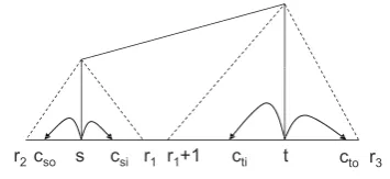
Figure 10 shows the structure of decision

his-tory of a left dependency (between s and t)

re-lation. For the right case, the structure is

simi-lar. In the figure,SHI is chart item[s, r1,→, C],

T HI is chart item [r1 + 1, t,←, C], SHO is

chart item[r2, s,←, C], and T HO is chart item

[t, r3,→, C]. We usecsi,cti,cso, andctoto

repre-sent a child ofs/tin subtreesSHI,T HI,SHO,

andT HOrespectively. The lexical form features

ofFSHIandFSHOare listed as examples in Table

1, where “L” refers to the left direction. We can also expand the nodes in the templates to the POS tags. Compared with the algorithm of Carreras (2007) that only considers the furthest children of

sandt, Algorithm 2 considers all the children.

Table 1: Lexical form features ofFSHIandFSHO

template FSHI FSHO

C+DIR word-csi+L word-cso+L C+DIR+S word-csi+L+word-s word-cso+L+word-s C+DIR+T word-csi+L+word-t word-cso+L+word-t C+DIR word-csi+L word-cso+L +S+T +word-s+word-t +word-s+word-t

4.4 Policy of using history

In practice, we define several policies to use the history information for different word pairs as fol-lows:

• All: Use the history-based features for all the

word pairs without any restriction.

• Sub-sentences: use the history-based

fea-tures only for the relation of two words from sub-sentences. Here, we use punctuation marks to split sentences into sub-sentences.

• Distance: use the history-based features for

(7)

5 Experimental results

In order to evaluate the effectiveness of the history-based features, we conducted experiments on Chinese and English data.

For English, we used the Penn Treebank (Mar-cus et al., 1993) in our experiments and the tool

“Penn2Malt”3_{to convert the data into dependency}

structures using a standard set of head rules (Ya-mada and Matsumoto, 2003a). To match previous work (McDonald and Pereira, 2006; Koo et al., 2008), we split the data into a training set (sec-tions 2-21), a development set (Section 22), and a test set (section 23). Following the work of Koo et al. (2008), we used the MXPOST (Ratnaparkhi, 1996) tagger trained on training data to provide part-of-speech tags for the development and the test set, and we used 10-way jackknifing to gener-ate tags for the training set.

For Chinese, we used the Chinese Treebank

(CTB) version 4.04 _{in the experiments. We also}

used the “Penn2Malt” tool to convert the data and created a data split: files 1-270 and files 400-931 for training, files 271-300 for testing, and files 301-325 for development. We used gold stan-dard segmentation and part-of-speech tags in the CTB. The data partition and part-of-speech set-tings were chosen to match previous work (Chen et al., 2008; Yu et al., 2008).

We measured the parser quality by the unla-beled attachment score (UAS), i.e., the percentage

of tokens with the correct HEAD5_{. And we also}

evaluated on complete dependency analysis. In our experiments, we implemented our

sys-tems on the MSTParser6 _{and extended with}

the parent-child-grandchild structures (McDonald and Pereira, 2006; Carreras, 2007). For the base-line systems, we used the first- and second-order (parent-sibling) features that were used in Mc-Donald and Pereira (2006) and other second-order features (parent-child-grandchild) that were used in Carreras (2007). In the following sections, we call the second-order baseline systems Baseline

3_{http://w3.msi.vxu.se/˜nivre/research/Penn2Malt.html} 4_{http://www.cis.upenn.edu/˜chinese/.}

5_{As in previous work, English evaluation ignores any}

to-ken whose gold-standard POS tag is one of{´´ `` : , .}and Chinese evaluation ignores any token whose tag is “PU”.

6_{http://mstparser.sourceforge.net}

and our new systems OURS.

5.1 Results with different feature settings In this section, we test our systems with different settings on the development data.

Table 2: Results with different policies

Chinese English Baseline 89.04 92.43

D1 88.73 92.27

D3 88.90 92.36

D5 89.10 92.59

D10 89.32 92.57

Dsub 89.57 92.63

Table 2 shows the parsing results when we used different policies defined in Section 4.4 with all

the types of features, whereDsubrefers to

apply-ing the policy: sub-sentence,D1 refers to

apply-ing the policy: all, andD₃_|₅_|₁₀refers to applying

the policy: distance with the predefined distance 3, 5, or 10. The results indicated that the accu-racies of our systems decreased if we used the history information for short distance words. The

system withDsubperformed the best.

Table 3: Results with different types of Features

Chinese English Baseline 89.04 92.43 +FSHI 89.14 92.53 +FT HI 89.33 92.35 +FSHO 89.25 92.47 +FT HO 88.99 92.54

Then we investigated the effect of different types of the history-based features. Table 3 shows

the results with policyDsub. From the table, we

found that FT HI provided the largest

improve-ment for Chinese andFT HO performed the best

for English.

In what follows, we usedDsubas the policy for

all the languages, the featuresFSHI +FT HI +

FSHO for Chinese, and the features FSHI +

FSHO+FT HO for English.

5.2 Main results

(8)

Chi-Table 4: Results for Chinese

UAS Complete

Baseline 88.41 48.85

OURS 89.43(+1.02) 50.86

OURS+STACK 89.53 49.42

Zhao2009 87.0 –

Yu2008 87.26 –

STACK 88.95 49.42

Chen2009 89.91 48.56

nese and 0.29 points for English. The improve-ments of (OURS) were significant in McNemar’s

Test withp <10−4 for Chinese andp <10−3for

English.

5.3 Comparative results

Table 4 shows the comparative results for Chinese, where Zhao2009 refers to the result of (Zhao et al., 2009), Yu2008 refers to the result of Yu et al. (2008), Chen2009 refers to the result of Chen et al. (2009) that is the best reported result on this data, and STACK refers to our implementa-tion of the combinaimplementa-tion parser of Nivre and Mc-Donald (2008) using our baseline system and the

MALTParser7_{. The results indicated that OURS}

performed better than Zhao2009, Yu2008, and STACK, but worse than Chen2009 that used large-scale unlabeled data (Chen et al., 2009). We also implemented the combination system of OURS and the MALTParser, referred as OURS+STACK in Table 4. The new system achieved further im-provement. In future work, we can combine our approach with the parser of Chen et al. (2009).

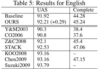
Table 5 shows the comparative results for En-glish, where Y&M2003 refers to the parser of Ya-mada and Matsumoto (2003b), CO2006 refers to the parser of Corston-Oliver et al. (2006), Z&C 2008 refers to the combination system of Zhang and Clark (2008), STACK refers to our implemen-tation of the combination parser of Nivre and Mc-Donald (2008), KOO2008 refers to the parser of Koo et al. (2008), Chen2009 refers to the parser of Chen et al. (2009), and Suzuki2009 refers to the parser of Suzuki et al. (2009) that is the best reported result for this data. The results shows that OURS outperformed the first two systems that were based on single models. Z&C 2008 and STACK were the combination systems of

graph-7_{http://www.maltparser.org/}

Table 5: Results for English

UAS Complete

Baseline 91.92 44.28

OURS 92.21 (+0.29) 45.24 Y&M2003 90.3 38.4

CO2006 90.8 37.6

Z&C2008 92.1 45.4

STACK 92.53 47.06

KOO2008 93.16 –

Chen2009 93.16 47.15

Suzuki2009 93.79 –

based and transition-based models. OURS per-formed better than Z&C 2008, but worse than STACK. The last three systems that used large-scale unlabeled data performed better than OURS.

6 Related work

There are several studies that tried to overcome the limited feature scope of graph-based depen-dency parsing models .

Nakagawa (2007) proposed a method to deal with the intractable inference problem in a graph-based model by introducing the Gibbs sampling algorithm. Compared with their approach, our ap-proach is much simpler yet effective. Hall (2007) used a re-ranking scheme to provide global fea-tures while we simply augment the feafea-tures of an existing parser.

Nivre and McDonald (2008) and Zhang and Clark (2008) proposed stacking methods to com-bine graph-based parsers with transition-based parsers. One parser uses dependency predictions made by another parser. Our results show that our approach can be used in the stacking frameworks to achieve higher accuracy.

7 Conclusions

(9)

References

Buchholz, S., E. Marsi, A. Dubey, and Y. Kry-molowski. 2006. CoNLL-X shared task on multilingual dependency parsing. Proceedings of CoNLL-X.

Carreras, X. 2007. Experiments with a higher-order projective dependency parser. In Proceedings of the CoNLL Shared Task Session of EMNLP-CoNLL 2007, pages 957–961.

Chen, WL., D. Kawahara, K. Uchimoto, YJ. Zhang, and H. Isahara. 2008. Dependency parsing with short dependency relations in unlabeled data. In Proceedings of IJCNLP 2008.

Chen, WL., J. Kazama, K. Uchimoto, and K. Torisawa. 2009. Improving dependency parsing with subtrees from auto-parsed data. In Proceedings of EMNLP 2009, pages 570–579, Singapore, August.

Corston-Oliver, S., A. Aue, Kevin. Duh, and Eric Ring-ger. 2006. Multilingual dependency parsing using bayes point machines. InHLT-NAACL2006. Culotta, A. and J. Sorensen. 2004. Dependency tree

kernels for relation extraction. In Proceedings of ACL 2004, pages 423–429.

Eisner, J. 1996. Three new probabilistic models for dependency parsing: An exploration. In Proc. of COLING 1996, pages 340–345.

Hall, Keith. 2007. K-best spanning tree parsing. In Proc. of ACL 2007, pages 392–399, Prague, Czech Republic, June. Association for Computational Lin-guistics.

Koo, T., X. Carreras, and M. Collins. 2008. Simple semi-supervised dependency parsing. In Proceed-ings of ACL-08: HLT, Columbus, Ohio, June. Li, Charles N. and Sandra A. Thompson. 1997.

Man-darin Chinese - A Functional Reference Grammar. University of California Press.

Marcus, M., B. Santorini, and M. Marcinkiewicz. 1993. Building a large annotated corpus of En-glish: the Penn Treebank. Computational Linguis-ticss, 19(2):313–330.

McDonald, R. and J. Nivre. 2007. Characterizing the errors of data-driven dependency parsing models. InProceedings of EMNLP-CoNLL, pages 122–131. McDonald, R. and F. Pereira. 2006. Online learning of approximate dependency parsing algorithms. In Proc. of EACL2006.

McDonald, Ryan. 2006. Discriminative Training and Spanning Tree Algorithms for Dependency Parsing. Ph.D. thesis, University of Pennsylvania.

Nakagawa, Tetsuji. 2007. Multilingual dependency parsing using global features. In Proceedings of the CoNLL Shared Task Session of EMNLP-CoNLL 2007, pages 952–956.

Nakazawa, T., K. Yu, D. Kawahara, and S. Kurohashi. 2006. Example-based machine translation based on deeper NLP. InProceedings of IWSLT 2006, pages 64–70, Kyoto, Japan.

Nivre, J. and R. McDonald. 2008. Integrating graph-based and transition-graph-based dependency parsers. In Proceedings of ACL-08: HLT, Columbus, Ohio, June.

Nivre, J., J. Hall, and J. Nilsson. 2004. Memory-based dependency parsing. In Proc. of CoNLL 2004, pages 49–56.

Nivre, J., J. Hall, S. K¨ubler, R. McDonald, J. Nilsson, S. Riedel, and D. Yuret. 2007. The CoNLL 2007 shared task on dependency parsing. In Proceed-ings of the CoNLL Shared Task Session of EMNLP-CoNLL 2007, pages 915–932.

Ratnaparkhi, A. 1996. A maximum entropy model for part-of-speech tagging. InProceedings of EMNLP, pages 133–142.

Suzuki, Jun, Hideki Isozaki, Xavier Carreras, and Michael Collins. 2009. An empirical study of semi-supervised structured conditional models for depen-dency parsing. In Proc. of EMNLP 2009, pages 551–560, Singapore, August. Association for Com-putational Linguistics.

Yamada, H. and Y. Matsumoto. 2003a. Statistical de-pendency analysis with support vector machines. In Proceedings of IWPT2003, pages 195–206. Yamada, H. and Y. Matsumoto. 2003b. Statistical

de-pendency analysis with support vector machines. In Proceedings of IWPT2003, pages 195–206. Yu, K., D. Kawahara, and S. Kurohashi. 2008.

Chi-nese dependency parsing with large scale automati-cally constructed case structures. InProceedings of Coling 2008, pages 1049–1056, Manchester, UK, August.

Zhang, Y. and S. Clark. 2008. A tale of two parsers: Investigating and combining graph-based and transition-based dependency parsing. In Pro-ceedings of EMNLP 2008, pages 562–571, Hon-olulu, Hawaii, October.