Differential propagation analysis of K
Joan Daemen and Gilles Van Assche
STMicroelectronics
Abstract. In this paper we introduce new concepts that help read and understand low-weight differential trails in K . We then propose efficient techniques to exhaustively generate all 3-round trails in its largest permutation below a given weight. This allows us to prove that any6-round differential trail in K -f[1600]has weight at least74. In the worst-case diffusion scenario where the mixing layer acts as the identity, we refine the lower bound to82 by systematically constructing trails using a specific representation of states.
Keywords:cryptographic hash function, K , differential cryptanalysis, computer-aided proof
1 Introduction
The goal of cryptanalysis is to assess the security of cryptographic primitives. Finding a acks or properties not present in ideal instances typically contributes to the cryptanalysis of a given primitive. Building upon previous results, a acks can be improved over time, possibly up to a point where the security of the primitive is severely questioned.
In contrast, cryptanalysis can also benefit from positive results that exclude classes of a acks, thereby allowing research to focus on potentially weaker aspects of the primitive. Interestingly, weaknesses are sometimes revealed by challenging the assumptions underlying positive results. Nevertheless, both a acks and positive results can be improved over time and together contribute to the understanding and estimation of the security of a primitive by narrowing the gap between what is possible to a ack and what is not.
Differential cryptanalysis (DC) is a discipline that a empts to find and exploit predictable dif-ference propagation pa erns to break iterative cryptographic primitives [6]. For ciphers, this typi-cally means key retrieval, while for hash functions, this is the generation of collisions or of second preimages. The basic version makes use of differential trails (also called characteristics or differ-ential paths) that consist of a sequence of differences through the rounds of the primitive. Given such a trail, one can estimate its differential probability (DP), namely, the fraction of all possible input pairs with the initial trail difference that also exhibit all intermediate and final difference when going through the rounds.
A more natural way to characterize the power of trails in unkeyed primitives is by their weight w. In general the weight of a trail is is the sum of the weight of its round differentials, where the la er is the negative of its binary logarithm. For many round functions, including that of K -f and Rijndael, the weight equals the number of binary equations that a pair must satisfy to follow the specified differences. Assuming that these conditions are independent, the weight of the trail relates to its DP asDP=2−wand exploiting such a trail becomes harder as the weight increases. For a primitive with, say,binput and output bits, the number of pairs that satisfy these conditions is then2b−w. The assumption of independence does not always apply. For instance, a trail withw>b implies redundant or contradictory conditions on pairs, for which satisfying pairs may or may not exist. Another example where this independence assumption breaks down are the plateau trails that occur in Rijndael [9]. These trails, with weight starting fromw=30for 2 rounds, have a DP equal to2z−wwithz>0for a fraction2−zof the keys and zero for the remaining part. In general, they occur in primitives with strong alignment [3] and a mixing layer based on maximum-distance separable (MDS) codes.
examples include a lower bound on the number of active S-boxes in JH [17] or computer-aided proofs on the weight of trails in N [7] and on the minimum number of active AND gates in MD6 [16,13].
K is a sponge function submi ed to the SHA-3 contest [15,4,2]. Recently, new results were published on the differential resistance of this function and among those heuristic techniques were proposed to build low-weight differential trails [11,14]. These gave the currently best trails for 3, 4 and 5 rounds of the underlying permutation K -f[1600]. In particular, Duc et al. found a trail of weight32for3rounds, and this motivated us to systematically investigate whether trails of lower weight exist. Also, there are some similarities between K and MD6, but unlike MD6, the permutation used in the proposed SHA-3 candidate K has no significant lower bounds on the weight of trails. So the philosophy behind [16,13] was another source of inspiration and motivation for our research.
Lower bounds on symmetric trails were already proven in [4]. They provide lower bounds with weight above the permutation width on K -f[25]to K -f[200]but only partial bounds in the case of K -f[1600]. Thanks to the Matryoshka structure [4], a lower boundWon trails in K -f[25w]implies a lower boundW′ =Www′ onw-symmetric trail in K -f[25w′]for w′>w. These are summarized in Table 1.
wLower bound forK -f[25w]Lower bound forK -f[1600]
1 30 per 5 rounds 1920 per 5 rounds tight
2 54 per 6 rounds 1728 per 6 rounds tight
4 146 per 16 rounds 2336 per 16 rounds non-tight
8 206 per 18 rounds 1648 per 18 rounds non-tight
Table 1.Lower bounds above the permutation width on1- to8-symmetric trails [4].
In this paper, we report on techniques to efficiently generate all the trails in K -f[1600] up to a given weight. We implemented these techniques in a computer program, which allowed us at this point to completely scan the space of3-round differential trails up to weight36. This confirmed that the trail found by Duc et al. has minimum weight and allowed us to demonstrate that there are no6-round trails with weight below74. These results are summarized in Table 2. The source code of the classes and methods used in this paper is available in the K T package [5].
As a by-product of this trail search, this paper proposes new techniques to relate the properties of theθmapping in K to the weight of differential trails. In the worst-case diffusion scenario whereθacts as the identity, we build upon the results of [4] and [14] to systematically construct so-called in-kernel trails using an efficient representation of states.
Rounds Lower bound Best known
3 32(this work) 32[11]
4 - 134(Appendix B)
5 - 510[14]
6 74(this work) 1360[4]
24 296(this work)
-Table 2.Weight of differential trails in K -f[1600].
Further discussions on how to exploit differential trails in K can be found in [3]. Also, the a acks in [10] combine algebraic techniques with a differential trail.
trails of K . Section 4 sets up the overall strategy and Section 5 introduces a basic trail gen-eration technique. The advanced techniques are covered in Sections 6 and 7, which address two complementary cases. Finally, Section 8 extends the results from3to6rounds.
2 K
K combines the sponge construction with a set of seven permutations denoted K -f[b], withbranging from25to1600bits [1,4]. In this paper, we concentrate on the permutation used in the SHA-3 submission, namely, K -f[1600].
The state of K -f[1600]is organized as a set of5×5×64bits with(x,y,z)coordinates. The coordinates are always considered modulo5forxandyand modulo64forz. Arowis a set of5bits with given(y,z)coordinates, acolumnis a set of5bits with given(x,z)coordinates and asliceis a set of25bits with givenzcoordinate.
The round function of K -f[1600]consists of the following steps, which are only briefly summarized here. For more details, we refer to the specifications [4].
– θis a linear mixing layer, which adds a pa ern that depends solely on the parity of the columns of the state. Its properties with respect to differential propagation will be detailed and ex-ploited in Section 6.
– ρandπdisplace bits without altering their value. Jointly, their effect is denoted by(x,y,z)−→π◦ρ (x′,y′,z′), with(x,y,z)a bit position beforeρandπand(x′,y′,z′)its coordinates a erward. – χis a degree-2non-linear mapping that processes each row independently. It can be seen as
the application of a translation-invariant5-bit S-box. The differential propagation properties will be detailed below.
– ιadds a round constant. As it has no effect on difference propagation, we will ignore it in the sequel.
3 Representing and extending trails
In general, for a function f with domainZb2, we define theweightof a differential(u′,v′)as
w(u′→f v′) =b−log2{u : f(u)⊕f(u⊕u′) =v′}.
If the argument of the logarithm is non-zero (i.e., the DP is non-zero), we say thatu′ andv′ are compatible. Otherwise, the weight is undefined.
The weight of a trail is the sum of the weight of the differentials that compose this trail. In K -f, we specify differential trails with the differences before each round function. For clarity, we adopt a redundant description by also specifying the differences before and a er the linear stepsλ=π◦ρ◦θ. Ann-round trail is of the following form, where eachbimust be equal toλ(ai),
Q=a0 π◦ρ◦θ
−→ b0→χ a1 π◦ρ◦θ
−→ b1→χ a2 π◦ρ◦θ
−→ . . . →χ an, (1) and has weightw(Q) = ∑iw(ai
χ◦π◦ρ◦θ
−→ ai+1). Sincebi = λ(ai), this expression simplifies to
w(Q) =∑iw(bi χ
→ai+1).
3.1 Extending forward and trail prefixes
Given a trail as in (1), it is possible to characterize all states that are compatible withbn = λ(an) throughχand thus to find alln+1-round trailsQ′that haveQas its leading part. This process is calledforward extension.
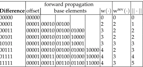
forward propagation
Differenceoffset base elements w(·)wrev(·)|| · ||
00000 00000 0 0 0
00001 00001 00010 00100 2 2 1
00011 00001 00010 00100 01000 3 2 2 00101 00001 00010 01100 10000 3 2 2 10101 00001 00010 01100 10001 3 3 3 00111 00001 00010 00100 01000 10000 4 2 3 01111 00001 00011 00100 01000 10000 4 3 4 11111 00001 00011 00110 01100 11000 4 3 5
Table 3.Space of possible output differences, weight, minimum reverse weight and Hamming weight of all row differences, up to cyclic shi s.
w(b)can also be computed on each row independently and summed. To constructA(b), the bases resulting from each active row are gathered. Table 3 displays offsets and bases for the affine spaces of all single-row differences.
As a consequence, the weight of an-round trailQisw(Q) =∑i=0n−1w(bi)and depends only on then-tuple(b0, . . . ,bn−1). We call the la er atrail prefix. Alln-round trails sharing this trail prefix and withancompatible withbn−1throughχhave the same weight.
3.2 Extending backward and trail cores
Similarly, given a trail as in (1), it is possible to construct all states that are compatible witha0 throughχ−1and thus to find alln+1-round trailsQ′that haveQas its trailing part. This process is calledbackward extension. In contrast to χ, its inverse has algebraic degree3and the space of compatible differences is not an affine variety in general. Yet, compatible values can be identified per active row and combined.
For a differenceaa erχ, we define theminimum reverse weightwrev(a)as the minimum weight over all compatiblebbeforeχ. Namely,
wrev(a)≜ min
b:a∈A(b)w(b).
Like for the restriction weight, the minimum reverse weightwrev(a)can be computed on each row independently and summed. Values are also shown in Table 3.
Given an−1-round trail prefixQ= (b1, . . . ,bn−1), it is easy to construct a differenceb0such that the trail prefixQ′ = b0||Qhas weight given byw(Q′) = w(Q) +wrev(λ−1(b1)). This is the smallest possible weight an-round trail can have withQas its trailing part. It follows that a sequence ofn−1state valuesQ˜ = (b1, . . . ,bn−1)defines a set ofn-round trails with a weight at least
˜
w(Q˜)≜wrev(λ−1(b1)) + n−1
∑
i=1
w(bi).
We denote the former by the termtrail coreand the la er by its weight. Note that an-round trail core is determined by onlyn−1states, although its weight takesnindividual weights into account.
K T implements the representation of trails, trail prefixes and trail cores (see theTrail
class), as well as the forward and backward extension (see theKeccakFTrailExtensionclass) [5].
4 Towards a bound for trails in
K
-
f
[
1600
]
To find a lower bound on differential trail weights in K -f[1600], our strategy is the following.
– Second, we derive a lower bound, not necessarily tight, on the weight of6-round trails by using the3-round trails found. Any6-round trail of weight2T3+1or less satisfies eitherw(b0) +
w(b1) +w(b2) ≤ T3or w(b3) +w(b4) +w(b5) ≤ T3. We thus use forward and backward extension from3-round trails up to weight2T3+1. If such trails are found, the one with the smallest weight defines the lower bound, which is naturally tight. Otherwise, this establishes a lower bound for the weight of6-round trails to2T3+2. In the la er case no trail with weight
2T3+2is known so the bound is not necessarily tight.
The reason for targeting3-round trails in the first phase is the following. The minimum weight of a1-round trail is 2, with a single active bit in b0. For the24rounds of K -f[1600], this amounts to a lower bound of24×2 =48. Constructing a stateawith only two active bits in the same column leads to2-round trail core with weight8. Hence, if we base ourselves only on2-round trail, we reach a lower bound of12×8 =96. If the3-round trail of weight32found by Duc et al. [11] has minimum weight, this would mean that a24-round trail has weight at least8×32=256. Also,3-round trail cores can be constructed by taking into account conditions across one layer of χ. Generating exhaustively trails of4rounds or more up to some weight would probably yield be er bounds, but at the same time it is more difficult as several layers ofχmust be dealt with. Instead, the two-step approach described above can take advantage of the exhaustive set of trails covered (i.e., all up to weightT3) to derive a bound based onT3instead of on the minimum weight over3rounds.
4.1 Generating all3-round trails up to a given weight
In our approach we generate all3-round differential trails of the form
Q=a0 π◦ρ◦θ
−→ b0→χ a1 π◦ρ◦θ
−→ b1→χ a2 π◦ρ◦θ
−→ b2→χ a3, (2)
up to some weight limitw(Q)≤ T3. We call this the target space. We do this by searching for all trail cores(b1,b2)with weight belowT3. Each such trail core(b1,b2)thus represents a set3-round trails of the form of Eq. (2) with weight not below that of its core. In the scope of this paper, we limited ourselves toT3=36.
We covered the set of all3-round trails up to weightT3in three sub-phases:
1. In Section 5, we start with all cores such thatwrev(λ−1(b1))≤7,w(b1)≤7orw(b2)≤7. 2. In Section 6, we generate all remaining cores, except where botha1anda2are in the kernel. 3. In Section 7, we finish by generating all cores where botha1anda2are in the kernel.
4.2 Too many states to generate and extend, even when exploiting symmetry
A way to generate all trails in the target space is to first generate all states up to a given weight and then do backward and forward extensions to obtain trail cores. If we defineT1≜
⌊ T3
3 ⌋
, then
forw˜(b1,b2)≤T3eitherwrev(λ−1(b1))≤T1,w(b1)≤T1orw(b2)≤T1. To cover the target space, we need to consider these cases:
– wrev(λ−1(b
1)) ≤ T1, so we have to generate all statesa1withwrev(a1) ≤ T1, computeb1 = λ(a1)and extend forward the2-round trail cores(b1)to get3-round trail cores.
– w(b1) ≤ T1, so we have to generate all statesb1 withw(b1) ≤ T1 and extend forward the
2-round trail cores(b1).
– w(b2) ≤ T1, so we have generate all states b2with w(b2) ≤ T1 and extend backward the
2-round trail cores(b2).
Unfortunately, this brute-force strategy requires a high number of states to cover the whole space for an interesting target weight. E.g., ifT3=36, thenT1=12and there are about1.42×1015≈250 states with weight up to12in K -f[1600].
alongz. Hence, for each trailQ= (b0,b1, . . . ,bn)there exists a trailQ′ = (z(b0), z(b1), . . . , z(bn)) of same weight, withzthe translation operator along the zaxis. In the sequel, we will always consider trails up to translations inz. This reduces the search space by approximately a factor w=64—not exactly a factorwbecause of states that are periodic inz. Yet, the number of states to extend forward and backward is still about244.
5 Generating trails with a low number of active rows
In this section, we generate and extend states with weight up toT1′ = 7. This does not cover the whole target space withT3= 36but the remaining portion of the target space is limited to trails with a more flat weight profile, i.e., they satisfyw(bi) ≥ T1′+1 = 8 for alli ∈ {0, 1, 2}and
w(bi) +w(bi+1)≤T2′ =T3−(T1′+1) =28for alli∈ {0, 1}.
More specifically, in this phase we look at the number of active rows in order to generate all trail cores such thatwrev(λ−1(b
1)) ≤ T1′,w(b1) ≤ T1′ orw(b2) ≤ T1′, forT1′ = 7. According to Table 3, each active row contributes for at least2to the weight. Hence,
w(b)≥2∥b∥row and wrev(b)≥2∥b∥row,
and we can cover all the states up to weight7by generating all states with up to⌊T1′
2⌋=3active rows.
This approach can be refined by looking at the number of active rows not only for one state but for two consecutive states. Withχ, the minimum weight a round differential can have is2. So,wrev(λ−1(b1)) ≥2implies thatwrev(λ−1(b2)) +w(b2) ≤w(b1) +w(b2) ≤ T3−2 = 34and similarlyw(b2)≥2implies thatwrev(λ−1(b1)) +w(b1)≤T3−2=34. Hence,
wrev(λ−1(bi)) +w(bi)≤T3−2=34 ⇒ ∥λ−1(bi)∥row+∥bi∥row≤ ⌊
T3−2
2
⌋ =17.
In practice, what we did was the following.
– GenerateB ={b : (∥b∥row ≤3or∥λ−1(b)∥row≤3)and∥λ−1(b)∥row+∥b∥row ≤17}. This is done by first generating all statesbwith up to 3 active rows and filter on∥λ−1(b)∥row, and then generate all statesawith up to 3 active rows, computeb=λ(a)and filter on∥b∥row. – Do forward extension of allb1∈ Band keep the coresQ˜ = (b1,b2)withw˜(Q˜)≤T3. – Do backward extension of allb2∈ Band keep the coresQ˜ = (b1,b2)withw˜(Q˜)≤T3.
We found a trail core(b1,b2)withwrev(λ−1(b1)) +w(b1) +w(b2) =4+4+24=32(see also Table 4). It contains the 3-round trail found by Duc et al. [11], of which a trail prefix is displayed in Figure 3 in Appendix A.
There are(320n )(31)n states withnactive rows. As this function grows very quickly, it was not reasonable to extend this search beyond3active rows.
The generation of trail cores based on a small number of active rows is implemented in the
KeccakFTrailCoreRowsclass [5].
6 Generating trails using the properties of
θ
To investigate the remaining part of the target space, we look at the properties of statesawith respect toθ, and specifically the parity of its columns, to limit the weight of two-round trails. An important parameter to classify the statesais their column parity, so as to study states in sets of parities. From the column parity, we derive theθ-gap, defined below. Withθ-gapg, the effect ofθ is to flip10gbits. There are thus at least10gactive bits, each either inaor inθ(a). So, the higher the θ-gap the higherwrev(a) +w(λ(a))is likely to be. We can efficiently compute a lower bound for
wrev(a) +w(λ(a))over allawith a given parity. For the target weights considered in this paper, this allows us to limit the states to consider to those with a parity belonging to a mere handful of values.
immediately be excluded. An important case is when all the columns ofahave even parity, i.e., ais in the kernel. In this case, theθ-gap is zero and a high number of states must be generated and extended. For this reason, this section focuses only the case where eithera1ora2is not in the kernel. The complementary case is covered in Section 7.
6.1 Properties ofθ
Asθis a linear function, its properties are the same whether applied on a state absolute value or on a difference, so we just write “value”. The following definitions are from [4].
Thecolumn parity(orparityfor short)P(a)of a valueais defined as the parity of the columns ofa, namelyP(a)[x][z] =∑ya[x][y][z]. A column iseven(resp.odd) if its parity is 0 (resp. 1). The parity can also be defined on a slice, namelyP(az)[x] =∑ya[x][y][z]. When the parity of a state or of a slice is zero (i.e., all its columns are even), we say it is in thecolumn-parity kernel(orkernelfor short).
The mappingθconsists in adding a pa ern to the state, which we call theθ-effect. Theθ-effect of a valueaisE(a)[x][z] =P(a)[x−1][z] +P(a)[x+1][z−1]. For a fixedθ-effecte[x][z],θcomes down to adding they-symmetric pa erne[x][y][z] ≜ e[x][z](∀y). Soθdepends only on column parities and always affects columns symmetrically iny.
A column of coordinates(x,z)isaffectediffE(a)[x][z] =1; otherwise, it isunaffected. Note that theθ-effect always has an even Hamming weight so the number of affected columns is even.
Theθ-gapis defined as the Hamming weight of theθ-effect divided by two. Hence, if theθ-gap of a value at the input ofθisg, the number of affected columns is2gand applyingθto it results in10gbits being flipped.
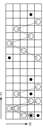
We have introduced theθ-gap via theθ-effect, but it can be defined directly using the parity itself. For this we introduce an alternative, single-dimensional, representation of a parityp[x][z]. We map the(x,z)coordinates to a single coordinatetast → (x,z) = (−2t,t)and denote the result byp[t]. In this representation arunis a sequence of ones delimited by zeroes. As illustrated on Figure 1, each run induces two affected columns. First, if it starts in coordinates(x,z), it implies an affected column in its right neighbor(x+1,z). And if it ends in(x′,z′)it implies an affected column in its top-le neighbor(x′−1,z′+1). Another example can be found in Figure 3. The following lemma links the number of runs to theθ-gap.
Lemma 1. The parityphasθ-gapgiffp[t]hasgruns.
6.2 The propagation branch number
Thepropagation branch numberof a parityp is the minimum weight of the2-round trail core(b) among states with this parity. More formally,
B(p)≜min{w˜(b) : P(λ−1(b)) = p}.
Owing to the portion of the target space already covered in Section 5, we can limit the propagation branch number toT2′ =28. The strategy is as follows:
– First, we identify and exclude parity pa ernspsuch that the propagation branch number can be proven to exceedT2′ =28.
– Then, for the remaining parity pa ernspwe look for all statesb = λ(a)withP(a) = pand
˜
w(b)≤T2′ =28.
– Finally, we forward and backward extend the states seen as2-round trail cores up to weight T3=36.
Clearly, the kernel states, i.e., states such thatP(a) =0must be considered. For instance, a state awith just two active bits in the same column will havewrev(a) =4. Then,b= λ(a) =π(ρ(a)) sinceθhas no effect in this case, andbalso has two active bits. For K -f[1600], all the rotation constants inρare different and these two bits will not be in the same slice, so not in the same row andwrev(a) +w(b) =8. Hence, the propagation branch number of the all-zero parity is at least8
and thus the all-zero parity pa ern must be included.
z
x
Fig. 1.Example of parity pa ern. Each square represents a column. An odd column contains a circle, while an affected column is denoted by a dot. A column can be both odd and affected. The odd columns of a run are connected with a line. The affected columns due to a run are located at the right (resp. top le ) of the start (resp. end) column of the run.
6.3 Bounding the row branch number
Therow branch numberof a parity p is the minimum number of active rows before and a erλ among states with this parity. More formally,
Brows(p)≜min{∥λ−1(b)∥row+∥b∥row : P(λ−1(b)) = p}.
Since an active row has at least propagation weight2, this means thatB(p) ≥2Brows(p). We can thus use the row branch number as a way to limit the search to parity pa erns for whichw˜(b)≤T2′. For a given parity pa ern, we classify the columns as either affected, unaffected odd or unaf-fected even. We make use of the following properties to find a lower bound on the row branch number.
Lemma 2. In terms of active rows,θsatisfies the following properties:
– An active bit in an affected column beforeθ will be passive a er θ, and vice-versa. So, for each bit
(x,y,z)−→π◦ρ (x′,y′,z′)of an affected column, at least one of row(y,z)inλ−1(b)and row(y′,z′)in bwill be active.
– An odd unaffected column always contains at least one active bit and this bit stays active a erθ. So, for at least one bit(x,y,z) −→π◦ρ (x′,y′,z′)of an odd unaffected column, both rows(y,z)inλ−1(b)and
(y′,z′)inbwill be active.
These properties are translated into Algorithm 1, which returns a lower bound ofBrows(p). The algorithm avoids counting twice an active row by marking (in the setsaandb) the row positions already encountered.
6.4 Looking for candidate parity pa erns
To find trails such that any two consecutive rounds have weight up toT2′ =28, we have to consider the parity pa erns listed in Lemma 3.
Lemma 3. A2-round differential trailQ= (b0,b1,b2)inK -f[1600]withw(Q)≤28necessarily
Algorithm 1Computing a lower bound ofBrows(p) Letaandbbe sets of row positions, which are initially empty B←0
for eachaffected column(x,z)do fory∈Z5do
Let(x,y,z)−→π◦ρ (x′,y′,z′) if(y,z)∈/aand(y′,z′)∈/bthen
B←B+1
a←a∪ {(y,z)}andb←b∪ {(y′,z′)} end if
end for end for
for eachunaffected odd column(x,z)do Let(x,i,z)−→π◦ρ (xi′,y′i,z′i)fori∈Z5 if{(i,z),i∈Z5} ∩a=∅then
B←B+1
a←a∪ {(i,z),i∈Z5} end if
if{(y′i,z′i),i∈Z5} ∩b=∅then B←B+1
b←b∪ {(y′i,z′i),i∈Z5} end if
end for return B
– a1is in the kernel, i.e.,P(a1) =0;
– theθ-gap ofa1is1with a single run of length1or2; or
– theθ-gap ofa1is2or3with runs of length1each, all starting in the same slice.
If parities are considered up to translation alongz, we can restrict ourselves to parity pa erns with runs starting in slicez=0.
To prove this result, we conducted a recursive search as follows. Each parity is represented as a set of runs. First, all parity pa ernspwith a single run (soθ-gap1) are investigated. Allpwith Brows(p) ≤ T
′ 2
2 = 14are stored into a setS. Then, we recursively add runs not overlapping the already added ones (so as to coverθ-gaps higher than1), and all foundpwithBrows(p)≤ T
′ 2 2 =14 are stored into a setS.
To limit the search, we use the following monotonicity property on the number of active rows. Using Lemma 2, changing an unaffected even column into either an unaffected odd or an affected column cannot decrease the number of active rows.
In the recursive search described above, adding a run to a parity pa ern p can turn an un-affected odd column into an un-affected column. Hence, we cannot use the monotonicity property directly on the runs. However, adding a run never turns an affected column back into an unaf-fected one. So, before recursively adding a run top, we apply a modified version of Algorithm 1 that does not take unaffected odd columns into account; this modified algorithm is monotonic in the runs. If the value returned by this modified algorithm is already above T2′
2 =14, then there is no need to further add runs. This efficiently cuts the search.
Before being added to the candidate setS, the parity pa ernpis tested with the unmodified Algorithm 1. For the remaining parity pa erns, we explicitly generated all states awith these parities up tow˜(λ(a))≤T2′ =28. This allowed us to prove Lemma 3.
Algorithm 1 is implemented in thegetLowerBoundTotalActiveRowsfunction and the recursive search inlookForRunsBelowTargetWeight[5].
6.5 Starting from out-of-kernel states
– In a first phase, we generate all statesasuch thatP(a) =pby assigning all possible16values to affected (odd or even) columns and by assigning a single active bit in each unaffected odd column. These states are such that||a||+||λ(a)||is exactly10g+2c, withgtheθ-gap andc the number of unaffected odd columns.
– In a second phase, we take the states generated in the first phase and add pairs of bits to all unaffected columns. By adding a pair of bits, we do not alterP(a).
In both phases, we keep only the statesb=λ(a)for whichw˜(b)≤T2′ =28. As can be seen in Table 3, both the weight and the reverse minimum weight aremonotonic, i.e., adding an active bit to the state cannot decrease them. We can therefore limit the search by stopping adding pairs of bits whenw˜(b)is aboveT2′ =28.
In practice, what we did was the following.
– LetPbe the set of parity pa erns satisfying one of the conditions of Lemma 3 exceptp=0. – By the method described above, we construct all states in the setB = {b : P(λ−1(b)) ∈
Pandw˜(b)≤T2′ =28}.
– Finally, we forward and backward extend the states inBto3-round trail cores up to weight T3=36.
We again found the same trail core as in Section 5. The trail prefix of weight32hasP(a1) =0 (soa1is in the kernel) andP(a2)has one run of length2(soa2hasθ-gap1). No other trail cores were found.
When extending the states inB, we exhaustively scan all compatible states, thereby including cases whereP(a1) =0orP(a2) =0. Hence, we covered the whole target space, except for trails such that bothP(a1) =0andP(a2) =0.
7 Generating in-kernel trails
To close the target space, we must look at in-kernel trails of the form in Eq. (2) with bothP(a1) =0 andP(a2) =0. In the case of in-kernel trails, we were able to be completely cover the space up to weightT3=40, and we expect the techniques presented here can cover trails of higher weight. As P(a1) =P(a2) =0, theθoperation has no effect and thereforebi=π(ρ(ai)). So this comes down to looking for statesa=a1,b=b1,c=a2andd=b2connected as:
a−→π◦ρ b→χ c−→π◦ρ d, withP(a) =P(c) =0. (3) We now summarize how we can efficiently generate all in-kernel three-round trail cores up to some weight and provide more details in following subsections. The key element in our method is the observation that any statebwithP(a) =0and for which there exists a statecwithP(c) =0
can be represented in a specific way. The statesaandbare iteratively constructed by adding active bits in the form of bit sequences called chains and vortices, defined in Section 7.2 below. Chains and vortices have an even number of active bits per column inaby construction and hence ensure P(a) =0.
Inb, there can be zero, one or more slices called knots, which contain three or more active bits. Each of these active bits is the end point of a chain that leads to another knot or that connects back to the same knot. The intermediate active bits of a chain appear pairwise in slices holding exactly two active bits in one column (called orbital slices, see Section 7.1). On top of chains connecting knots, a statebcan exhibit a vortex, i.e., a cyclic sequence of active bits that appear pairwise both in the columns ofaand in the columns ofb.
By starting with an empty state and progressively adding chains, knots and vortices, one can quickly build statesaandbthat satisfyP(a) =0and for which there existcwithP(c) =0, leading to3-round in-kernel trail cores. Any state leading to a in-kernel trail can be represented in this way, and care is taken so that all possible states are generated, up to a given target weight. At each step, a lower bound on the weight of3-round trail cores containingaandbis computed so as to efficiently limit the search.
7.1 Characterizing the slices inb
Definition 1. A statebistameifP(λ−1(b)) =0and such that there exists at least one stateccompatible withbthroughχsuch thatP(c) =0.
To characterize statesbsuch thatP(c) = 0, we can reason on the slicesbzofbsinceχandP can be jointly described in terms of slices. In particular, each sliceczofcmust be in the kernel, namely,P(cz) =0, and we have to characterize the slicesbzunder that constraint. First, ifbz =0 thencz=0andP(cz) =0. Then, a slicebzwith a single active bit cannot be in the kernel a erχ, as at least one column ofczwill have a single active bit. Finally, a slicebzwith two active bits must have its two active bits in the same column forczto be in the kernel. By inspection of Table 3, a row with a single active bit at coordinatex, e.g.,00100transforms into an active row of the formuv100
withu,v∈ {0, 1}, so the active bit stays active atxand zero, one or two active bits can appear at x−2andx−1of the same row. So, if the two bits are not in the same column, one of the active bits that stays a erχwill not find another active bit in the same column. We summarize this in the next lemma.
Lemma 4. Ifbis tame, then each of its slices has either
– no active bit,
– two active bits in the same column, or – three or more active bits.
We call anempty slicea slice with no active bit, and anorbital sliceis a slice with two active bits in the same column. A slice that is neither empty not an orbital slice is called aknot. We say that a knot istameif it can transform a erχinto a slice in the kernel. According to Lemma 4, a tame knot has at least three active bits.
7.2 Characterizing the set of active bits
Since in the kernelθacts as the identity, the active bits ofaare just moved to other positions inb and their number remains the same, i.e.,||a||=||b||. We can therefore representaandbby a list of active bit positions(pi)i=1...||a||in either the coordinates(xi,yi,zi)inaor the coordinates(x′i,y′i,z′i) inb, with(xi,yi,zi)
π◦ρ
−→(xi′,y′i,zi′).
First, we start with the active bits ina. We say that active bitspiand pjarepeerif they are in the same column ina, i.e.,xi = xjandzi = zj. Since each column has an even number of active bits whenP(a) =0, an active bit thus always has a peer.¹
Then, we move to the active bits inb. We say that the two active bits pi andpjarechainedif they both lie in the same orbital slice inb. Sox′i =x′jandz′i =z′jand no other active bit is in slice z′i.
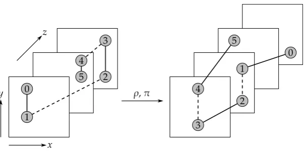
Achainis a sequence of bit positions of even length(p0,p1,p2, . . . ,p2n−1)such that p2k and p2k+1are peer (∀k∈ {0, . . . ,n−1}) and that p2k+1andp2k+2are chained (∀k ∈ {0, . . . ,n−2}). In addition, the first and last active bits p0and p2n−1must be in knots (either the same one or different ones). The simplest possible chain has length2and consists only in two peer active bits. Figure 2 depicts the concept of chain.
The definition of avortexis the same as that of a chain(p0,p1,p2, . . . ,p2n−1), except that the first and last active bitsp0and p2n−1must be chained. In other words, a vortex forms a cycle of bit positions linked alternatively by peer and chained relationships, all in orbital slices.
In a tame state, each active bit position has exactly one peer position. The active bit positions in knots are the end points of chains, while the active bits in orbital slices are chained and belong to chains or vortices. Therefore, any tame state can be represented as a set of vortices and chains connecting knots.
0 1 2 3 4 5 y x z ρ, π 0 1 2 3 4 5
Fig. 2.Schematic example of a chain. An active bit position is represented by a circle with its index. Two active bits connected by a plain line (resp. dashed line) are peer (resp. chained).
7.3 Generating all tame states
To generate all tame states up to a target weightT3, we generate statesaandbby representing them using the concepts of Sections 7.1 and 7.2. The generation builds (initially empty) statesa andbby iterating the following nested loops:
– In the outer loop, we add chains to the existing state. When adding a chain(p0,p1,p2, . . . ,p2n−1), the slices that receive the end pointsp0andp2n−1must become knots if they are not already. If n>1, the pairs of (chained) active bits(i2k+1,i2k+2)are added to empty slices, which become orbital slices. Active bits cannot be added to already constructed orbital slices, as it would contradict the definition of an orbital slice. Enough chains must be added such that each knot contains at least3active bits (see Lemma 4).
– For a fixed set of chains produced in the previous step, the inner loop iterates on the number and position of vortices. In a vortex, all active bits are chained, so they must be added to empty slices, which become orbital slices.
With the monotonic lower bound function defined in the next section, we add chains and vortices until this lower bound exceedsT3.
7.4 Lower-bounding the weight of in-kernel trails
We wish to determine a lower bound on the weight of3-round in-kernel trail cores(b,d), namely, onwrev(a) +w(b) +w(d) witha = λ−1(b), from aandbonly, for use in our trail generation. Since onlydis unknown, this implies finding a lower bound onw(d). This can be done by first determining a lower bound on the Hamming weight||d||and then bounding the weight of any state with given Hamming weight.
To determine a lower-bound on||d||, we work on each slice ofb. If slicebzhasu = ∥bz∥row active rows, then the slicecz has at leastu active bits. In addition, P(cz) = 0 implies that the number of active bits must be even, so||cz|| ≥2⌈u2⌉. Finally, we have||d||=||c||so
||d|| ≥2
∑
z ⌈
∥bz∥row
2
⌉
.
From Table 3, it is easy to verify the following lower bound:
w(d)≥wˆ(||d||)≜ ⌈
4||d||
5
⌉
+ [1if||d||=1or2 (mod 5)].
Hence, we define thelower weightofbas
L(b)≜wrev(λ−1(b)) +w(b) +wˆ
(
2
∑
z ⌈
∥bz∥row
2
⌉)
Numberw˜(·)wrev(b1)w(b1)w(b2) P(a1) P(a2)Structure ofa1,b1
1 32 4 4 24kernelθ-gap1
1 35 12 12 11kernel kernel vortex of length6 7 36 12 12 12kernel kernel vortex of length6 7 39 12 12 15kernel kernel vortex of length6
2 39 12 11 16kernel kernel2knots connected by3chains 41 40 12 12 16kernel kernel vortex of length6
4 40 12 12 16kernel kernel2knots connected by3chains
Table 4.Summary of all3-round differential trail cores found in K -f[1600]up to weight36, and up to weight40for in-kernel trails. The number indicates the number of cores with the same properties indicated in the other columns.
The lower weight yields a lower bound on the weight of3-round in-kernel trail cores(b,d) regard-less ofd.
7.5 Limiting the search by lower-bounding the weight
At each level of the loop described in Section 7.3, the corresponding iteration is aborted, and el-ements are not further added, if we can be sure that the lower weightL(b)will become larger than the target weightT3. Adding a chain to the state can potentially bring new knots and/or new orbital slices. Adding a vortex necessarily brings new orbital slices. Therefore, there is a limit in the number of knots and orbital slices that must be considered for the generation to be complete up to the target weight.
As a preliminary step, the minimum reverse weight satisfies the following inequality (see Ta-ble 3):
wrev(a)≥wˆrev(||a||)≜ ⌈
3||a||
5
⌉
.
We see from Lemma 4 that each tame knot contributes to at least3active bits in aand in b. Furthermore, the number of bits in each slice ofamust be even (P(a) = 0), so||a|| ≥ 2
⌈ 3k
2 ⌉
and
wrev(a)≥wˆrev(||a||), withkthe number of knots. Inb, each tame knot has at least3active bits on at least2different active rows, hence contributing at least5to the weight, and sow(b)≥5k. Each active row inbcontributes to at least one active bit indso||d|| ≥2kandw(d)≥wˆ(||d||).
For instance,k=5knots implies that||a|| ≥16andwrev(a)≥wˆrev(16) =10, thatw(b)≥25
and that||d|| ≥10andw(d)≥wˆ(10) =8, so a lower weight of at least43. IfT3≤42, looking for configurations with from0to4knots is therefore sufficient, not even counting the orbital slices that also compose chains.
We found cores of weight35,36,39and40, as detailed in Table 4. For illustration purposes, examples of trail prefixes are shown in Figures 4, 5 and 6 in Appendix A. The search described in this section is implemented in theTrailCore3RoundsandTrailCoreInKernelAtCclasses [5].
8 Extension to six-round trails
Table 4 summarizes all the3-round cores found. These trail cores completely represent all the
3-round trails up to weight36(or40for in-kernel trails). They can be found in [5].
The second phase introduced in Section 4 consists in exhaustively extending forward and back-ward all the3-round trail cores into6-round trails cores. As no6-round trail of weight up to73
were found, we conclude that a6-round differential trail in K -f[1600] has at least weight
74. In the specific case of in-kernel trails, no6-round trail of weight up to81were found and we conclude that a6-round in-kernel differential trail in K -f[1600]has at least weight82.
9 Conclusions
We studied and implemented the exhaustive generation of3-round differential trails in the K -f[1600] permutation, which allowed us to prove a lower bound on the weight of differential trails. The techniques developed in this paper exploit the properties of the mixing layer in its round function to provide be er bounds than what a brute-force method could provide. Table 2 shows that there remains a gap between the best known trails and the lower bound beyond three rounds that calls for future work. Finally, the concepts introduced in this paper, such as chains, vortices, knots and parity runs, help read trails and understand them.
References
1. G. Bertoni, J. Daemen, M. Peeters, and G. Van Assche,On the indifferentiability of the sponge construction, Advances in Cryptology – Eurocrypt 2008 (N. P. Smart, ed.), Lecture Notes in Computer Science, vol. 4965, Springer, 2008,http://sponge.noekeon.org/, pp. 181–197.
2. ,Cryptographic sponge functions, January 2011,http://sponge.noekeon.org/. 3. ,On alignment inK , ECRYPT II Hash Workshop 2011, 2011.
4. ,TheK reference, January 2011,http://keccak.noekeon.org/. 5. , K T so ware, April 2012,http://keccak.noekeon.org/.
6. E. Biham and A. Shamir,Differential cryptanalysis of DES-like cryptosystems, CRYPTO (A. Menezes and S. Vanstone, eds.), Lecture Notes in Computer Science, vol. 537, Springer, 1990, pp. 2–21.
7. J. Daemen, M. Peeters, G. Van Assche, and V. Rijmen,Nessie proposal: the block cipherN , Nessie submission, 2000,http://gro.noekeon.org/.
8. J. Daemen and V. Rijmen,The design of Rijndael — AES, the advanced encryption standard, Springer-Verlag, 2002.
9. ,Plateau characteristics and AES, IET Information Security1(2007), no. 1, 11–17.
10. I. Dinur, O. Dunkelman, and A. Shamir,New a acks on Keccak-224 and Keccak-256, Fast So ware Encryp-tion 2012, 2012, to appear, dra available from Cryptology ePrint Archive, Report 2011/624.
11. A. Duc, J. Guo, T. Peyrin, and L. Wei,Unaligned rebound a ack: Application to Keccak, Fast So ware En-cryption 2012, 2012, to appear, dra available from Cryptology ePrint Archive, Report 2011/420. 12. P. Gauravaram, L. R. Knudsen, K. Matusiewicz, F. Mendel, C. Rechberger, M. Schläffer, and S. S. Thomsen,
Grøstl – a SHA-3 candidate, Submission to NIST (round 3), 2011.
13. E. Heilman,Restoring the differential security of MD6, ECRYPT II Hash Workshop 2011, 2011.
14. M. Naya-Plasencia, A. Röck, and W. Meier,Practical analysis of reduced-round Keccak, Indocrypt 2011, 2011. 15. NIST,Announcing request for candidate algorithm nominations for a new cryptographic hash algorithm (SHA-3) family, Federal Register Notices72(2007), no. 212, 62212–62220,http://csrc.nist.gov/groups/ST/hash/ index.html.
16. R. Rivest, B. Agre, D. V. Bailey, S. Cheng, C. Crutchfield, Y. Dodis, K. E. Fleming, A. Khan, J. Krishna-murthy, Y. Lin, L. Reyzin, E. Shen, J. Sukha, D. Sutherland, E. Tromer, and Y. L. Yin,The MD6 hash function – a proposal to NIST for SHA-3, Submission to NIST, 2008,http://groups.csail.mit.edu/cis/md6/. 17. H. Wu,The hash function JH, Submission to NIST (round 3), 2011.
A Some three-round differential trails
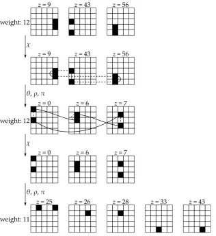
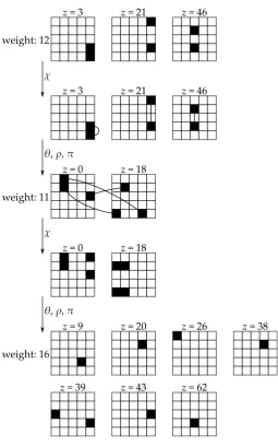
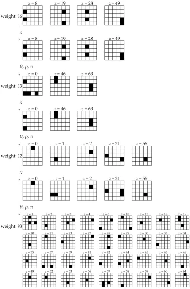
In this section, we give some examples of trails for illustration purposes. In the figures, trail pre-fixes are depicted withb0,a1,b1,a2,b2 from top to bo om as in Eq. (2) and the weight of each round is given beforeχ. The differenceb0 was taken such thatw(b0) = wrev(a1). At each step, only the slices with non-zero difference are shown with theirzcoordinate. Thexcoordinate goes from le to right withx = 0at the center, while theycoordinate goes from bo om to top with y=0at the center. Active bits are depicted in black.
When P(a1) = 0, the peer and chained relationships are shown with straight and dashed lines, respectively, as in Figure 2. Examples of structures include a vortex of length6, two knots connected by three chains, and one knot connected to itself by two chains. In Figure 3,P(a2)̸=0 and the effect ofθis illustrated in details.
B A four-round differential trail
z = 0
weight: 4
χ z = 0
θ, ρ, π
z = 55 z = 56
weight: 4
χ
z = 55 z = 56 z = 57
θ
z = 55 z = 56 z = 57
ρ, π
z = 0 z = 6 z = 14 z = 18 z = 21 z = 34
z = 48 z = 49 z = 52 z = 53 z = 57 z = 61 weight: 24
parity and θ-effect:
z
x
odd column affected column
z = 9 z = 43 z = 56
weight: 12
χ
z = 9 z = 43 z = 56
θ, ρ, π
z = 0 z = 6 z = 7
weight: 12
χ
z = 0 z = 6 z = 7
θ, ρ, π
z = 25 z = 26 z = 28 z = 33 z = 43
weight: 11
z = 3 z = 21 z = 46
weight: 12
χ
z = 3 z = 21 z = 46
θ, ρ, π
z = 0 z = 18
weight: 11
χ
z = 0 z = 18
θ, ρ, π
z = 9 z = 20 z = 26 z = 38
z = 39 z = 43 z = 62 weight: 16
z = 0 z = 21 z = 43 z = 54
weight: 16
χ
z = 0 z = 21 z = 43 z = 54
θ, ρ, π
z = 0 z = 18 z = 34
weight: 13
χ
z = 0 z = 18 z = 34
θ, ρ, π
z = 15 z = 35 z = 36 z = 38 z = 57 z = 62
weight: 12
z = 8 z = 19 z = 28 z = 49
weight: 16
χ
z = 8 z = 19 z = 28 z = 49
θ, ρ, π
z = 0 z = 46 z = 63
weight: 13
χ
z = 0 z = 46 z = 63
θ, ρ, π
z = 0 z = 1 z = 2 z = 21 z = 55
weight: 12
χ
z = 0 z = 1 z = 2 z = 21 z = 55
θ, ρ, π
z = 1 z = 2 z = 3 z = 4 z = 6 z = 10 z = 15 z = 18 z = 19
z = 20 z = 21 z = 23 z = 27 z = 28 z = 29 z = 30 z = 33 z = 34
z = 35 z = 37 z = 39 z = 41 z = 42 z = 44 z = 45 z = 46 z = 48
z = 49 z = 52 z = 53 z = 56 z = 57 z = 58 z = 59 z = 60 z = 61 weight: 93
![Table 1. Lower bounds above the permutation width on 1- to 8-symmetric trails [4].](https://thumb-us.123doks.com/thumbv2/123dok_us/7892307.1309820/2.595.172.424.583.658/table-lower-bounds-permutation-width-symmetric-trails.webp)
![Table 4. Summary of alland up to weight 3-round differential trail cores found in K�����-f [1600] up to weight 36, 40 for in-kernel trails](https://thumb-us.123doks.com/thumbv2/123dok_us/7892307.1309820/13.595.136.465.84.177/table-summary-alland-weight-dierential-weight-kernel-trails.webp)