Technology (IJRASET)
©IJRASET 2015: All Rights are Reserved
254
Optimization and Analysis of Vertical Axis Wind
Turbine Using Flow vision Solver
Mr. Shivakantgoud Hosagoudr1, Dr. S. Kumarappa2 1
Post Graduate student Thermal Power Engineering, 2Department of Mechanical Engineering, Bapuji Institute of Engineering and Technology, Davanagere, Karnataka, India.
Abstract: Wind energy is renewable source of energy and is available in nature. These days wind energy become most popular energy source. In present paper 3D models of VAWTs was designed with and without diffuser. The diffuser was designed to direct the wind towards the turbine blades to increase the wind velocity for more power generation. These models are analyzed by using computational fluid dynamics tools. All models are designed using Catia V5 and results of these models are presented. Keywords: Wind energy, VAWT, CFD, Flow-vision, 3D models.
I. INTRODUCTION
Wind energy outshines all other renewable energy resources due to the recent technological improvements. Electrical energy generation from wind power has increased rapidly and due to the increased interest many studies on efficient wind turbine design have been performed. In this study, a new wind turbine concept suitable for power generation at highway and low wind speeds is demonstrated. 3D models of VAWTs were designed with and without diffuser. The diffuser was designed to direct the wind towards the turbine blades to increase the wind velocity for more power generation. In this paper, performance analyses of the wind turbine models concept are performed and the results are summarized.
[image:2.612.215.394.384.707.2]II. METHODS AND METHADOLOGY
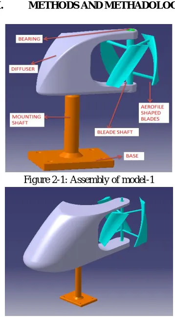
Figure 2-1: Assembly of model-1
Technology (IJRASET)
[image:3.612.218.395.81.235.2]©IJRASET 2015: All Rights are Reserved
255
Figure 2-3: Assembly of model-3
The above figure 2-1 is the assembly of model-1. These 3D models are designed in Catia v5 modeling software. In our model we have designed the diffuser for the purpose to direct the wind towards the airfoil shaped blades to increase the wind velocity and power generation. The diffuser design is also an airfoil to utilize more amount of wind which is being wasted at the entrance of diffuser. The blade dimensions are Height is 800mm, Diameter is 608mm, Thickness is 8mm, and Angle is 450. The shaft dimensions are Diameter is 25mm and length is 850mm. The base dimensions are Height is 152mm and Width is 880mm. The bearing diameter is 25mm.
In assembly of model-2 we used the same airfoil shaped blades but the dimensions of blades are changed as per the design of diffuser. In 2nd model we changed the diffuser design to increase the wind velocity. For that we have increased the radius of the diffuser at the entrance of the wind and also increased the thickness at the entrance. We made round shape design at entrance to increase the wind velocity and power generation. Here more outward diverting wind is directed towards the turbine blades. In model-3 we used the same airfoil shaped blades but changed dimensions of blades as per the design of diffuser. In this model we changed the diffuser design by making it straight with reduced thickness at the entrance of the wind. In each design we were changing the diffuser design to optimize the turbine which will give more power. In each model the blade shape is kept same in all the models.
A. Experimental Results Considered For The Analysis
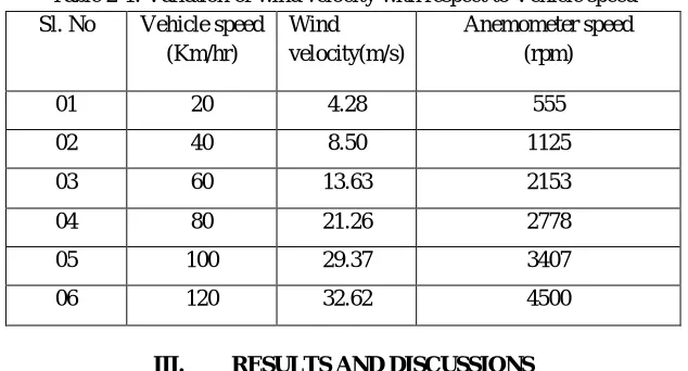
To determine the potential of wind prevailing at highways experiments were conducted at highway. Results obtained are shown in table 2.1. Vehicle speed and wind velocity were measured with the help of speedometer and anemometer.
Table 2-1: Variation of wind velocity with respect to Vehicle speed Sl. No Vehicle speed
(Km/hr)
Wind velocity(m/s)
Anemometer speed (rpm)
01 20 4.28 555
02 40 8.50 1125
03 60 13.63 2153
04 80 21.26 2778
05 100 29.37 3407
06 120 32.62 4500
III. RESULTS AND DISCUSSIONS
[image:3.612.148.465.510.681.2]Technology (IJRASET)
©IJRASET 2015: All Rights are Reserved
256
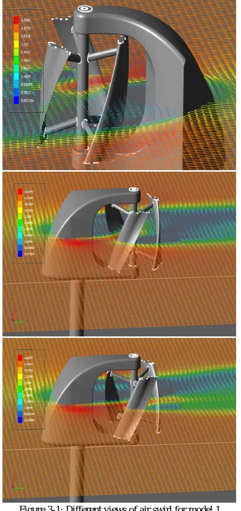
[image:4.612.184.430.90.611.2]1) Velocity 4.28m/s:
Figure 3-1: Different views of air swirl for model 1
Technology (IJRASET)
©IJRASET 2015: All Rights are Reserved
257
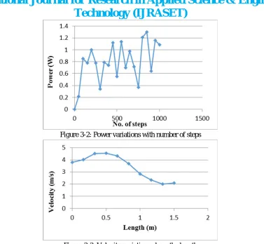
[image:5.612.120.497.49.397.2]Figure 3-2: Power variations with number of steps
Figure 3-3: Velocity variations along the length
The figure 3.2 shows the variations of power. We have considered the variation of power for every 50 steps. The power varies from one averaged 50 steps to another because of air swirl around the blades and some amount of air passing between the blades, it offers the resistance to rotation hence power is dropped. The power generated for velocity of 4.28m/s is 0.8W.
The figure 3.3 shows the variation of velocity along the length. Here we have considered the length from entrance of air at the diverging inlet to the air passes away after strikes on the blades surface. By using diverging section, wind velocity increases around 0.75m/s compared to normal wind velocity.
B. Velocity 8.50m/s:
[image:5.612.185.429.519.700.2]Technology (IJRASET)
[image:6.612.179.482.71.228.2]©IJRASET 2015: All Rights are Reserved
258
Figure 3-5: Velocity variations along the length
Figure 3.4 shows the variation of power with the number of steps. For velocity of 8.50 m/s, power generated is 2.29W. Figure 3.5 shows the variations of velocity along the length of the line, which is drawn from the inlet of diverging portion to the end of blades. The wind velocity increases to 1.53m/s were observed and hence power generation is also increases by using diffuser
[image:6.612.181.432.309.666.2]3) Velocity 13.63m/s:
Figure 3-6: Power variations with number of steps
Figure 3-7: Velocity variations along the length
Figure 3.6 shows the variation of power with the number of steps. Here the power is continuously varies from one step to another step. The power generated for this wind velocity is 8.03W.
Technology (IJRASET)
©IJRASET 2015: All Rights are Reserved
259
[image:7.612.181.432.90.427.2]4) Velocity 21.26m/s:
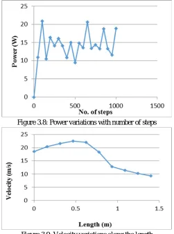
Figure 3.8: Power variations with number of steps
[image:7.612.184.429.544.712.2]Figure 3.9: Velocity variations along the length
Figure 3.8 shows the variations of power with the number of steps for velocity of 21.26 m/s. The power is continuously varies from one step to another because of air swirl and the air movements between the blades and shaft. For this velocity the power generated is 14.355W.
Figure 3.9 shows the variations of wind velocity along the length of line. The velocity increases at the diffuser around is 3.95m/s.
B. Model 2
1) Velocity 4.28m/s:
Technology (IJRASET)
©IJRASET 2015: All Rights are Reserved
260
(b)
[image:8.612.160.438.70.425.2](c)
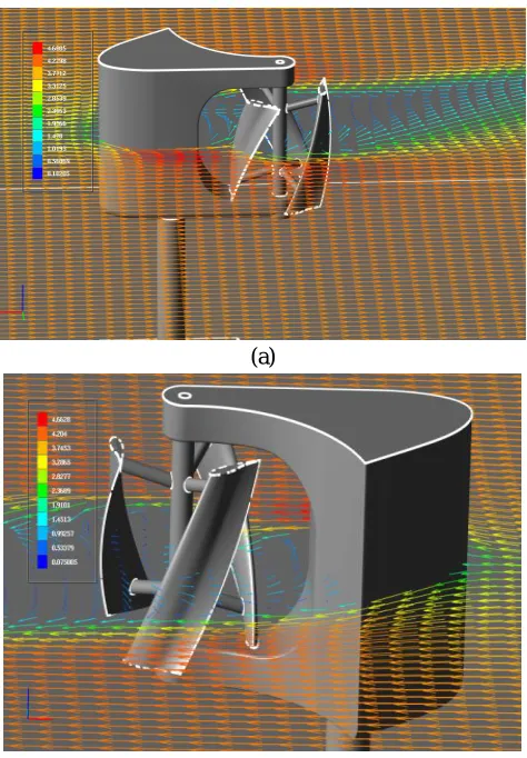
Figure 3-10: Different views of air swirl for model 2
Figure 3.10 shows the different views of air swirl around the blades. Figure 3.10 (a) shows the air swirl in Y plane, by keen observation of the picture, some amount of air moving along the blade rotation with velocity 1.6m/s. This is indicated by light blue color vectors. Figure 3.10 (b) shows the vectors of air movement in X plane, the air strike on the surface of blade and some amount of air moving back towards the diffuser which is indicated by blue color vectors. The velocity increases at the diffuser which is indicated by the red color vectors. Red color vectors show the maximum velocity at diffuser. Figure 3.10 (c) is another view of turbine assembly here air swirl between blades and shaft is less compared to model 1.
[image:8.612.183.428.535.713.2]Technology (IJRASET)
©IJRASET 2015: All Rights are Reserved
261
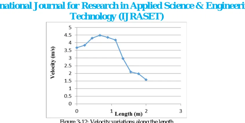
[image:9.612.105.528.39.252.2]Figure 3-12: Velocity variations along the length
The figure 3.11 shows the variation of power with the number of steps. The power generated is 1.01W for this velocity.
The figure 3.12 shows the variation of velocity along the length. For this model the wind velocity is increases around 0.81m/s at the diffuser, hence generate more power than the model 1.
2) Velocity 8.50m/s
Figure 3-13: Power variations with the number of steps
[image:9.612.184.432.73.248.2]Figure 3-14: Velocity variations along the length
[image:9.612.182.430.329.690.2]Technology (IJRASET)
©IJRASET 2015: All Rights are Reserved
262
Figure 3.14 shows the variation of velocity along the length. For this design of diffuser the wind velocity at entrance of it is increased around 1.62m/s.
[image:10.612.181.431.120.452.2]3) Velocity 13.63m/s
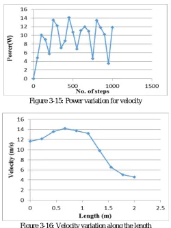
Figure 3-15: Power variation for velocity
Figure 3-16: Velocity variation along the length
Figure 3.15 shows the variation of power with number of steps. Power is varying from one step to another. For this velocity the average power is 10.208W.
Figure 3.16 shows the variation of velocity along the length. The velocity is decreasing after hitting the blade it is because of the kinetic energy of wind is extracted from turbine. Here velocity is increasing around 2.56m/s.
4) Velocity 21.26m/s
[image:10.612.183.431.541.691.2]Technology (IJRASET)
[image:11.612.160.486.66.249.2]©IJRASET 2015: All Rights are Reserved
263
Figure 3-18: Velocity variation along the length
[image:11.612.188.425.374.715.2]Figure 3.17 shows the power variation with number of steps. Here also power is varying from one step to another step. The power generated for this velocity is 26.345W.
Figure 3.18 shows the variation of velocity along the length. Here velocity is increasing around 4.08m/s. The maximum velocity is at the diffuser section and minimum is at the air movement after the striking on the blade surface where the energy in wind is harnessed from turbine blades
C. Model 3
1) Velocity 4.28m/s:
(a)
Technology (IJRASET)
©IJRASET 2015: All Rights are Reserved
264
(c)
Figure 3-19: Different views of air swirl for model 3
[image:12.612.84.513.33.230.2] [image:12.612.185.431.327.501.2]The above figures show the different views of air swirling around the blade area. Figure 3.19 (a) shows the air swirling around the blades in X plane here we can see the air stream towards the outlet of domain and some moving back towards the diffuser wall. Figure 3.19 (b) shows clearly the air movement towards the diffuser and some amount of air moving through the blades rotation velocity of these vectors is low. Figure 3.19 (c) shows the next step of (b) here we the air movement on the blades surface due to swirl at the diffuser, inside surface which is exposed to the blade side. In this model more power generate, since here air swirl and air movement between the blades is less compared to model 1.
[image:12.612.186.430.532.700.2]Figure 3-20: Power variation with the number of steps
Technology (IJRASET)
©IJRASET 2015: All Rights are Reserved
265
Figure 3.20 shows the variation of power with the number of steps for velocity 4.28m/s. We have obtained a power of 0.858W. Figure 3.21 shows the variations of velocity along the length of the line which is drawn from air entrance at the diffuser to air passing away from blades after blades rotation. In this case velocity is increased around 0.99m/s.
[image:13.612.183.431.136.486.2]2) Velocity 8.50m/s:
Figure 3-22 : Power variation with the number of steps
Figure 3-23: Velocity variation along the length
Figure 3.22 shows the variation of power with the number of steps for velocity 8.50m/s. We have gained a power of 3.36W. Figure 3.23 shows the variations of velocity along the length of the line. The velocity at the diffuser is increasing around 1.97m/s.
[image:13.612.188.428.547.710.2]3) Velocity 13.63m/s:
Technology (IJRASET)
[image:14.612.179.483.68.262.2]©IJRASET 2015: All Rights are Reserved
266
Figure 3-25: Velocity variation along the length
Figure 3.24 shows the variations of power with the number of steps. Here the power is varying because of air swirl around the blade area. The power generated is 8.78W.
Figure 3.25 shows the variations of velocity along with the length of the line. Here the velocity at the diffuser is increased around 3.06m/s.
4) Velocity 21.26m/s :
[image:14.612.181.430.346.705.2]Figure 3-26: Power variation with the number of steps
Technology (IJRASET)
©IJRASET 2015: All Rights are Reserved
267
Figure 3.26 shows the power variations with the number of steps Even here the power is varying continuously with number of steps. Figure 3.27 shows the velocity variations along the length of the line. The increased velocity for this model is around 4.23m/s.
[image:15.612.181.433.137.248.2]D. Comparison of Analytical Results
Table 3.1: Results of CFD analysis
Table 3.1 shows the analytical results of all models. For all wind velocities more power is generated using model 2 and model 3 for different wind velocities compared to model 1. Based on the CFD analytical results we conclude that model 2 is the best, which gives more power compared to model 1 and model 2. Considering model 3 gives us the more wind velocity at the diffuser compared to model 1 and model 2
1) Variation Of Power With Vehicle Speed:
[image:15.612.182.429.351.525.2]Figure 3-28: variation of power with vehicle speed
Figure 3.28 shows the variation of power with respect to vehicle speed. As we said earlier the power in model 2 is more compared to other two models and model 3 is producing more power than the model 1.
IV. CONCLUSION
From the results obtained, the following conclusions are made.
For velocity 4.28m/s the power increased in model 2 are 26.25% and 17.71% compared to model 1 and model 3 respectively. In model 3 power increased to 7.25% compared to model 1.
For velocity 8.50m/s power increased in model 2 are 91.7% and 30.65% compared to model 1 and model 3 respectively. In model 3 power increased to 46.72% compared to model 1.
For velocity 13.63m/s power increased in model 2 are 27.12% and 16.26% compared to model 1 and model 3 respectively. In model 3 power increased 9.38% compared to model 1.
For velocity 21.26m/s power increased in model 2 are 83.52% and 24.85% compared to model 1 and model 3 respectively. In model 3 power increased 46.98% compared to model 1.
Sl. No Vehicle speed (Km/hr) velocity (m/s) Power (W) Model 1 Model 2 Model 3
01 20 4.28 0.8 1.01 0.858
02 40 8.50 2.29 4.39 3.36
03 60 13.63 8.03 10.208 8.78
Technology (IJRASET)
©IJRASET 2015: All Rights are Reserved
268
REFERENCES
[1] Nilay Sezer-Uzol, Lyle N. Long “3-D Time-Accurate CFD Simulations of Wind Turbine Rotor Flow Fields”. American Institute of Aeronautics and Astronautics. published on 2006, AIAA paper no 2006-0394.
[2] Travis J. Carrigan, Brian H. Dennis, Zhen X. Han, and Bo P. Wang “Aerodynamic Shape Optimization of a Vertical-Axis Wind Turbine Using Differential Evolution”. International Scholarly Research Network ISRN Renewable Energy Volume 2012, Article ID 528418, 16 pages doi:10.5402/2012/528418.
[3] Habtamu Beri, Yingxue Yao “Double Multiple Stream Tube Model and Numerical Analysis of Vertical Axis Wind Turbine”. Energy and Power Engineering, 2011, 3, 262-270 doi: 10.4236/epe. 2011.33033 Published Online July 2011.
[4] Chris Kaminsky, Austin Filush, Paul Kasprzak, Wael Mokhtar “A CFD Study of Wind Turbine Aerodynamics”. American Society for Engineering Education, Proceedings of the 2012 ASEE North Central Section Conference.
[5] Dr.P.M.Ghanegaonkar, Ramesh K.Kawade, Sharad Garg “Conceptual Model of Vertical Axis Wind Turbine and CFD analysis” International Journal of Innovative Research in Advanced Engineering (IJIRAE), Volume 1 Issue 3(May 2014) SPECIAL ISSUE.