Machine Learning Optimisation for Realistic 2D and 3D PET CT Phantom Study

SCIENCEDOMAIN

international

Machine Learning Optimisation for Realistic 2D and 3D

PET-CT Phantom Study

Mhd Saeed Sharif

, Maysam Abbod

, Luke I Sonoda

and Bal Sanghera

1_{Department of Electronic and Computer Engineering, School of Engineering and Design, Brunel}

University, London, United Kingdom.

2_{Paul Strickland Scanner Centre, Mount Vernon Hospital, United Kingdom.}

Original Research

Article

Received: 31 May 2013 Accepted: 03 August 2013 Published: 20 November 2013

Abstract

An experimental study using artificial neural network (ANN) is carried out to achieve the optimal network architecture for proposed positron emission tomography (PET) application. 55 experimental phantom datasets acquired under clinically realistic conditions with different 2-D and 3-D acquisitions and image reconstruction parameters along with 2min, 3min and 4min scan times per bed are used in this study. The best scanner parameters are determined based on the ANN experimental evaluation of the proposed datasets. The analysis methodology of phantom PET data has shown promising results and can successfully classify and quantify malignant lesions in clinically realistic datasets.

Keywords: Image Analysis, Positron Emission Tomography (PET), Tumour, Segmentation, Artificial Neural Network

1

Introduction

A positron as the antimatter equivalent of an electron ( i.e. positive electron) is produced by radioactive decay and can be used in medical imaging. Positron emission tomography (PET) is a tomographic technique which is used to measure physiology and function rather than anatomy by imaging elements such as carbon, oxygen and nitrogen which have a high abundance within the human body. Among all diagnostic and therapeutic procedures, PET is unique in the sense that it is based on molecular and pathophysiological mechanisms and employs radioactively labeled biological molecules as tracers to

study the pathophysiology of the tumour in vivo to direct treatment and assess response to therapy. The leading current area of clinical use of PET is in oncology, where18_{F-fluorodeoxyglucose (FDG)} remains the most widely used tracer. It has already had a large valuable effect on cancer staging and treatment and its use in clinical oncology practice continues to evolve [1, 2]. PET imaging is utilised in the clinical specialities of oncology, cardiology and neurology.

PET has been mostly used to diagnose and determine treatments effectiveness for tumours in different parts of the human body such as lung, breast, head, neck and heart. In general, malignant cells have higher rates of aerobic glucose metabolism than healthy cells. As a result, tumours are depicted as regions of increased intensity. If patient lesions are spread from their original focus area, a whole body PET scan is performed. The patient is injected intravenously with FDG and placed in the scanner around 30 minutes up to 2 hours after injection [3, 4]. PET can be also used to monitor cerebral blood flow and glucose metabolism in diabetic patients [5, 6]. PET is used as well for staging, assessing residual disease and treatment response for patients with lymphoma [7, 8].

Analysing the volume data acquired from PET scanner is very important for different clinical applications including artefact reduction and removal, tumour quantification in staging, a process which analyses the development of tumours over time, and to aid in radiotherapy treatment planning [9, 10]. The utilisation of advanced high performance analysis software will be useful in aiding clinicians in diagnosis and radiotherapy planning. Although the task of medical volume analysis appears simple, the reality is that an in-depth knowledge of the anatomy and physiology is required to perform such tasks on clinical medical images. Essentially for each slice within a specified volume the clinical expert determines borders between regions and classifies each region using transaxial, sagittal and coronal slice information.In addition to this, identifying the features of small region of interest (ROI) in each slice and modifying the contrast are often required by the clinical experts. Despite the potential for lengthy visual analysis and uncertainty in complex cases, their manual analysis for a typical 3D data-set is considered as the most reliable and accurate method of medical volume analysis. This is due to the immense complexity of the human visual system, a system well suited to this task [11, 12, 13]. Analysing and extracting the proper information from PET volumes can be performed by utilising software analysis and classification approaches which provide richer information compared to what can be extracted from visual interpretation of the PET volumes alone. The need for accurate and fast analysis approaches of imaging data motivated the exploitation of artificial intelligence (AI) technologi-es. Artificial neural network (ANN) is one of the powerful AI techniques that has the capability to learn from a set of data and construct weight matrices to represent the learning patterns. ANN can be defined as an information processing system which contains a small/large number (according to the design and application) of highly interconnected processing units called neurons. This system has been inspired by the biological nervous system. The ANN components work at three levels, firstly they work together in a distributed manner to learn the input pattern (input information), secondly they coordinate internal processing, and finally optimise the final output.

Bayesian information criterion (BIC) were used to assess the optimal number of classes for each PET dataset. This paper is organised as follows: Section 2 presents theoretical background for the proposed approach with details regarding optimisation of neural network architecture. PET scanner methodology and characteristics are presented in section 3, the proposed medical slice analysis approach is described in section 4 with details of the ANN best architecture chosen. Results metrics between ANN of individual PET scans and the real phantom spheres with analysis are illustrated in section 5, and finally the conclusion of which PET clinical scanning parameters can best be represented by ANN analysis is highlighted in section 6.

2

Theoretical Background

Feedforward neural network (FFNN) is a mathematical model which emulates the activity of biological neural networks in the human brain. It has many interconnected group of neurons, each one of them has a number of inputs and one output. Those neurons are grouped in a finite number of layers with different types of connections between layers. The number of neurons in each layers is selected to be sufficient for solving the problem in question. Typically the network consists of input layer, a certain number of hidden layers, and outputs layer. The number of layers is desired to be minimal in order to decrease the problem solving time. FFNN is a supervised network, where the stimulus for learning comes from a teacher as the output of the neuron is compared against the known answer, i.e. the network targets. The neuron is trained with a representative subset of the processed data plus its suitable targets and if the training set, architecture, and learning approach are correct, the network will be able to generalise and solve the required problem. During the training phase the weights are adapted according to the discrepancy between the actual and desired output from the neuron in an attempt to bring the former one in line with the latter one. This stage is very important to achieve the training objective in term of correlating the input pattern with the desired targeted response. In other words, the rule will always converge to weights which accomplish the desired classification [16, 17, 18, 19, 20]. In this study the main neural network parameters have been investigated thoroughly at the beginning to obtain the optimal neural network architecture. The utilised design has been achieved based on the experiment done on different parameters as discussed in later sections.

2.1

Mathematical Model of a Neuron

The main element of the neural network is the neuron, which may work in two modes; the training mode and the evaluation mode. Each neuron in the network has a number of inputs (the input vector

X) and one output (Y). The input vector elements are multiplied by weightsw1,1,w1,2, ... ,w1,m ,

and the weighted values are fed to the summing junction. Their sum is simply the dot product (W.X) of the single row matricesW andX. The neuron has a biasb, which is summed with the weighted inputs to form the net inputn. This sum,n, is the argument of the transfer functionf[16]. An abstract model of an artificial neuron is illustrated in Figure 1.

n= m

∑

i=1

w1,i.xi+b (2.1)

Y =f(W.X+b) (2.2)

Y(j) =f[ m

∑

i=1

w1,i(j).xi(j) +b] (2.3)

The learning process can be summarised in the following steps:

Figure 1: Abstract model of an artificial neuron [21].

2. The neuron is activated by applying inputs vector and desired output (Yd).

3. The actual output (Y) is calculated at iterationj=1 as illustrated in Equation 2.3, where iteration

jrefers to thejth_{training example presented to the neuron.}

4. This step is to update the weights to obtain an output consistent with the training examples, this update can be done according to Equation 2.4.

w1,i(j+ 1) =w1,i(j) + ∆w1,i(j) (2.4)

where∆w1,i(j)is the weight correction at iterationj. The weight correction is computed by

using the delta rule in Equation 2.5.

∆w1,i(j) =α.xi(j).e(j) (2.5)

whereαis the learning rate. Different experiments have been carried out for different values of the learning rate and the most suitable value for PET application (which gives the least error) isα=0.6.e(j)is the error which can be given by the following equation.

e(j) =Yd(j)−Y(j) (2.6)

5. Finally, the iterationjis increased by one, and the previous two steps are repeated until the convergence is reached.

3

PET Scanner methodology and characteristics

PET imaging is a diagnostic imaging modality used to map the distribution of positron emitting radio-pharmaceutical agents within the human body. These agents are predominantly created using a cyclotron and are radioactive equivalents of biologically active molecules. A commonly used radio-pharmaceutical agent is FDG which contains 18_{F. This isotope undergoes radioactive decay} by emitting a positron and a neutrinov[4, 3].

A ZX −→

A

Z−1X+e +

+v (3.1)

are a consequence of the conservation of energy and momentum. The scanner contains hardware discriminators which automatically reject photons with energies that are considerably lower as this will be due to scattered radiation which causes noise in images.The two γ-rays travel in opposite directions at an angle of approximately180oto one another [3].

e++e−−→γ+γ (3.2)

The two γ-rays are detected by the detection system in the scanner, which is an entire ring of scintillation crystals that surround the patient. A schematic of a PET head scanner showing annihilation coincidences is illustrated in Figure 2 [4].

[a]

[b]

Figure 2: PET imaging detection system. (a) Transaxial view. (b) Anterior view

shows how radio-nuclides in a particular cross-sectional plane will be detected by

the rings of detectors [4].

detectors. In 2-D acquisition mode retractable septa are positioned between each ring enabling volume acquisition with collimation of signal, whereas in 3-D mode these septa are retracted. Image planes can be formed between two crystals in the same ring (direct planes), and also from crystals in adjacent rings (cross planes). For a system withnrings, there arendirect planes andn−1cross planes, making a total of2n−1image planes as illustrated in Figure 3. Then×nthree dimensional volume can be obtained when the septa are removed, the sensitivity of a 3-D acquisition can be ten times higher than that of the corresponding 2-D acquisition due to the absence of the septa [3].

Figure 3:

Different data acquisition modes in 2-D acquisition and 3-D PET

acquisition [3].

Both 2-D and 3-D acquisition modes lead to the creation of 3D data volumes following image reconstruction techniques. Following physical acquisition of data with 2-D or 3-D acquisition modes, image reconstruction techniques are employed to visualise the original radioisotope distribution within the patient’s body using projections of data acquired from the scanner detectors at different angles. A statistical image reconstruction technique called ordered subset expectation maximisation (OSEM) is used. In OSEM, a crude image estimate is initially generated and the corresponding estimated projection data is calculated, and then compared with the real measured projection data. Then, the image estimate is updated based on the ratio or difference between measured and estimated projections. This process is repeated for a number of iterations until satisfactory convergence of the algorithm is established. This technique is relatively fast as it splits the estimated and measured projections into subsets and updates the estimated image before the next subset commences. A full iteration has taken place if all subsets have been considered. Both 2-D and 3-D acquisition modes result in the reconstruction of 3D volumes of data for visualisation and quantitative analysis.

(FORE-WLS-OSEM) [24] and model based scatter correction [25]. Additional 2D and 3D corrections were performed for randoms (singles), decay, dead time, geometry and attenuation. In 2D imaging, a relatively uniform response across the detectors occurs, and many signals are rejected, especially from scattered events which degrade image quality. 3D imaging mode greatly increases the sensitivity of the PET scanner (typically bigger than 5 times) compared to 2D imaging with the acquisition of oblique events. The detector response in 3D is not uniform but it is more peaked. For adequate sampling, this requires more bed positions to be scanned for the same body sections. In 2D acquisition mode, patients may be scanned in five or six bed positions as they pass through the PET scanner, but in 3D mode, seven or eight beds position might be required. However, with 3D mode the PET system must be able to cope with the additional scattered radiation that degrades image quality. In addition the scanner must be able to cope with the extra signals being emitted from the patient. So, dead time (time required to process information) must be managed properly to avoid paralysis of the system. Furthermore the increase in the received signal will also contribute to a form of noise called randoms, which substantially increases as more signals are detected by the system.

Some large volumetric errors encountered using the acquisition systems exist due to the choice of systems variables, such as the slice thickness selected for the scan. The slice thickness can cause large fluctuations in accurately viewing and measuring transaxial tumour areas that can change the shape between image slices. This problematic characteristic occurs notably with small anatomical objects, such as the lesion in its early stages or the smallest spherical insert in NEMA IEC body phantom, where single voxel reallocation causes a large deviation in percentage error.

One of this study’s objectives is to attempt to define standards of using the PET scanner variables in the area of medical imaging. NEMA IEC body phantom has been used experimentally in this study. This phantom consists of an elliptical cavity housing six spherical inserts suspended by plastic rods of volumes 0.5, 1.2, 2.6, 5.6, 11.5, and 26.5 ml. The inner diameters of these spheres are: 10, 13, 17, 22, 28 and 37 mm. The PET attenuation corrected reconstructed image volume consists of 128 x 128 x 47 voxels, each voxel has dimensions of 4.6875 mm x 4.6875 mm x 3.27 mm corresponding to a volume of 0.0718 ml. The deployed NEMA IEC body phantom is illustrated in Figure 4 [26].

Figure 4: NEMA IEC body phantom containing six spheres [26].

each case, the generated cross sectional area using the developed ANN software has been analysed and compared with the cross sectional area acquired under standard clinical imaging conditions for the scanner.

In PET-CT scanning a ”whole body”, namely from orbit of the eyes to mid thigh, scan is acquired with fixed PET detectors as the patient moves through the scanner. In our system the PET detectors correspond to a bed position of about 16 cm transaxially, and a series of bed positions allow the entire body to be scanned. Each static bed position is scanned for a fixed time; the default is 4 minutes per bed position.

A standard clinical 2D imaging protocol with a 4min scan time per bed position is routinely used by the scanning centre providing the data here, with OSEM reconstruction utilising two iterations and 30 subsets. In 3D scanning, with no collimator, the OSEM reconstruction arbitrarily employs five iterations and 32 subsets as routine, with a 4min scan per bed acquisition. The other objective of this study is to investigate the efficiency of the proposed approach for segmenting lesions of different sizes (represented by spheres in the NEMA IEC body phantom), in a clinically realistic setting of relative activity levels and lesion diameters. The influence of the sphere size is investigated in both 2D and 3D, with OSEM reconstruction of varying iterations for a fixed 4min, 3min and 2min scan time/bed. This clinically realistic study was expected to optimise the capability of the developed proposed system for future clinical lesion detection with lesions of varying size and under different clinical environments.

4

The Proposed Approach

There are different parameters that should be investigated to build the proper approach based on ANN, such as the training approach, how many hidden layers should be used, and how many hidden neuron in each layer should be utilised. Beside that there are some other aspects should be considered during the primary experiment such as over-learning, over-fitting, or sometimes not having sufficient training examples. As the network with less weights may not be sufficiently powerful to model the underlying problem. For instance, a network with no hidden layers actually models a simple linear problem. However, a larger complex network will almost invariably achieve a lower error eventually, but this may indicate over-fitting rather than good modeling. Therefore a test subset data has been deployed to check the network progress. The number of hidden neuron has been also controlled to prevent network over-learning, where the error stops dropping, or indeed starts to rise. On the other hand if the error keeps high and not drops to the required level, this indicates insufficient network design. To add more confidence in the performance of the achieved model, a validation subset data has been deployed, where the final model has been evaluated with this set to ensure that the results on the testing and training set are real, and not artifacts of the training process.

Iterative experiments have been conducted 10 times with each network configuration, and the best architecture has been retained. This includes 9 inputs, 70 hidden neurons and 1 outputs. There are different activation functions have been investigated such as, hard limit, symmetrical hard limit, linear, saturating linear, symmetric saturating linear, log-sigmoid, and hyperbolic tangent sigmoid function [15, 16, 21]. Based on the initial investigation hyperbolic tangent sigmoid transfer function has been used for all layers except the output layer. Hyperbolic tangent sigmoid can be defined using Equation 4.1, and it is illustrated in Figure 5 (a). While the linear activation function has been selected for output layer, as linear transfer is sufficient for the classification purpose of different voxels into a distinct class. The deployed linear function (f(x) =x) is shown in Figure 5 (b).

a=e n₋

e−n

en_+e−n (4.1)

[a]

[b]

Figure 5: Activation functions: (a) Tangent-sigmoid function, (b) Linear function [21].

activation function, and the training approach. In general too few hidden units leads to high training error and high generalisation error due to under-fitting. However too many hidden units generate low training error but might associated with high generalisation error due to over-fitting. There are different rules implemented in the literature to obtain the best hidden neuron number. The first one states that this number should be between the input neurons numberNinand the output neurons numberNout, this method has been applied to the proposed PET application, however bad performance has been achieved in terms of the network performance error and the outputs error, both were high. The second rule indicates that the hidden neuron numberNhcan be calculated using the following formula.

Nh=

2∗(Nin+ Nout)

3 (4.2)

Based on this equation high training error has been achieved, therefore it has not led to the best number of hidden neurons for the proposed application. Others stated that just double the number of the inputs is enough as a hidden neurons number [16, 27, 28], also this method has not generated the proper number for the hidden neurons. Therefore doing the primary experiment is essential to obtain the optimal hidden neurons for the proposed PET analysis. In this experimental study multilayer FFNN consists of input layer, hidden layer (variant number of hidden neurons), and outputs layer has been chosen to determine the best number of hidden neurons. A window of size 3×3

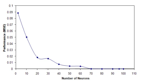
has been utilised in the neural network input, as this window considers the area of the neighbouring voxels, so the effect of the whole neighbouring voxels is considered. While utilising an input with one voxel has not given much information about the processed voxel. The outputs layer has one neuron. To evaluate the effect of the number of neurons in the hidden layer and achieve the best ANN performance for the proposed application, different numbers of neurons in the hidden layer have been used. The maximum number of iterations used in the neural network training is 1000. This number has been chosen based on the fact that the network can reach the steady state for all the training cases by using an iteration number equal to or less than 1000. The experiment has been repeated 10 times for each chosen number of the hidden neurons, and the average was considered for that number. Hyperbolic tangent sigmoid transfer function has been used for all layers except the output layer where the linear activation function is used. Levenberg-Marquardt backpropagation training algorithm [29] has been used during the evaluation of neurons numbers in the hidden layer to validate the best design for the ANN, which is suitable for the proposed PET application. Figure 6 presents the number of neurons in the hidden layer with the performance measured using mean squared error (MSE) based on 1000 iterations. The results obtained after this evaluation shows that the best number of the hidden neurons which corresponds to the smallest MSE, and good network outputs is 70 hidden neurons. Using two hidden layers has not added any significant performance value for the proposed application, it has just complicated the network architecture, and consumed more processing time. Therefore one hidden layer has been used in the proposed network design.

Figure 6: Evaluation of the number of neurons in the hidden layer with neural

network performance using MSE.

for each deployed training algorithm. The best outputs associated with the best performance was achieved using Levenberg-Marquardt backpropagation training algorithm.

5

The Results

5.1

Experimental Phantom Study

This study has utilised 55 PET acquired NEMA IEC volume datasets with a clinical GE DST PET-CT scanner, where each individual dataset consists of 47 slices. Some of these volume datasets have 2D acquisition, with the collimator in place, while other datasets have 3D acquisition without the collimator in place. Datasets were acquired for different times such as 2, 3 and 4 min. All the PET data is attenuation corrected (AC), except one dataset has non-attenuated PET data (PET NAC) used for a reference by clinicians in cases were attenuation may have introduced artefacts.

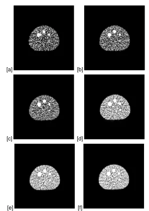
Figure 7 shows NEMA phantom slice acquired using 2D mode versus 3D mode for 2min, 3min and 4min acquisition time respectively. Changing the acquisition time as well as the acquisition mode have affected and altered the accuracy of the developed approach.

5.2

Results and Discussion

The experiment was evaluated based on the ratio between the combined spheres area (as ROI) to the remaining area of the scanned slice with the highest sphere diameters. The actual spheres area can be calculated according to equation 5.1, given that the spheres diameters are 10, 13, 17, 22, 28, 37 mm.

S= 1 4π

∑

r∈{a}

r2;{a}={10,13,17,22,28,37} (5.1)

[a]

[b]

[c]

[d]

[e]

[f]

Figure 7: NEMA phantom data using different acquisition modes and time (all at 15

iterations). (a, b, c) 2D acquisition at 2min, 3min and 4min respectively. (d, e, f) 3D

acquisition at 2min, 3min and 4min respectively.

equations 5.2 and 5.3 respectively; SBR is the sphere to the rest of the slice ratio.

A= 128×128×4.6875×4.6875 = 360000mm2 (5.2)

SBR= S

A−S ×100 = 0.7019% (5.3)

derived an error measure called absolute relative error defined as ARE = the absolute of (ANN PET measured value - phantom original) /phantom original. Table 1 illustrates SBR and ARE for different datasets with different scanner variables. It can be seen that the SBR percentages vary based on the used scanner variables. The 3D scans produce closer SBR percentages than 2D for all iterations except at iteration = 1. It can be noticed that the region of interest evaluating the spheres decreases as the iteration value increases for both 2D and 3D and for all bed section scanning times. This result matches the expectation of the radiologists.

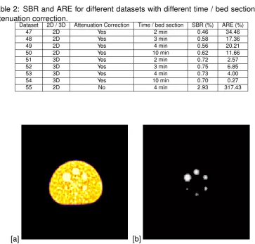
Table 2 shows the other datasets with different scanning time per bed section which also tested with attenuation correction and without attenuation correction. SBR and ARE of these datasets are also demonstrated in the same table. It can be seen that 3D is still much better than the 2D scan, and the quality is increased by increasing the time spent on each bed section in the scanning process. A very small error of 0.27% has been achieved for the dataset number 54 at 10 min bed section time. A big jump in the SBR can be noticed from the scanned dataset without attenuation correction (number 55) with a huge ARE. This is expected as the scanned output is blurred and very hard to analyse.

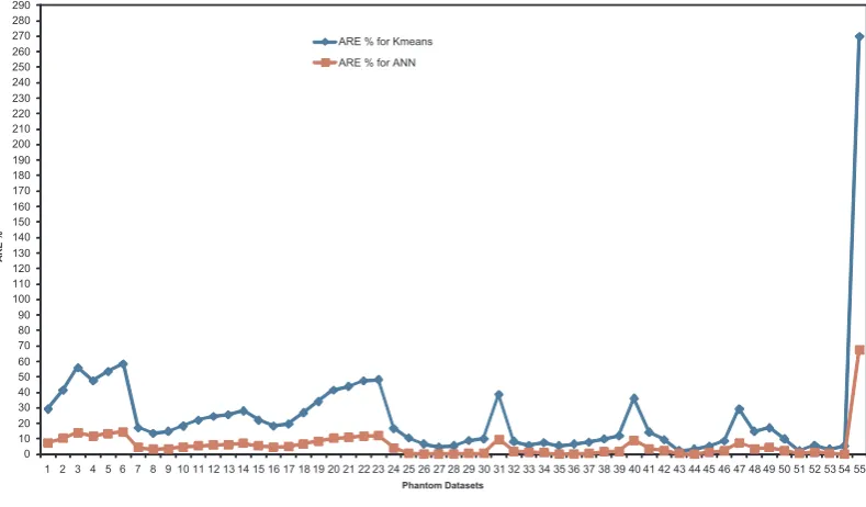
The proposed approach has been used to analysed all the phantom datasets. The best result has been achieved for the 3D datasets with iteration= 10, such as dataset number 35. An ARE%=0.27 has been achieved for this dataset. These results have been compared with the results achieved by using another classification approach based onkmeans and followed by thresholding approach. The best ARE% using this approach was 3.33 which is 12 times bigger that the ARE% achieved by the proposed approach. The worst ARE% was for dataset number 55 which has no attenuation correction. Figure 8 shows the ARE% results achieved for all the 55 datasets using the proposed ANN approach andKmeans. Figure 9.(a) presents original NEMA slice containing six spheres (128×128) from dataset number 54, and Figure 9.(b) illustrates the segmented slice (128×128) based on the ANN, where just the ROI is displayed.

3KDQWRP'DWDVHWV $5( $5(IRU.PHDQV $5(IRU$11

Table 1: SBR for different datasets with different scanner parameters.

Dataset 2D / 3D Iteration Subsets Time / bed section SBR (%) ARE (%) 1 2D 1 30 2 min 0.46 34.46 2 2D 3 30 2 min 0.36 48.71 3 2D 10 30 2 min 0.24 65.80 4 2D 20 30 2 min 0.31 55.83 5 2D 25 30 2 min 0.26 62.95 6 2D 30 30 2 min 0.22 68.65 7 2D 1 30 3 min 0.56 20.21 8 2D 5 30 3 min 0.59 15.94 9 2D 7 30 3 min 0.58 17.36 10 2D 10 30 3 min 0.55 21.64 11 2D 15 30 3 min 0.52 25.91 12 2D 20 30 3 min 0.50 28.76 13 2D 25 30 3 min 0.49 30.18 14 2D 30 30 3 min 0.47 33.03 15 2D 1 30 4 min 0.52 25.91 16 2D 3 30 4 min 0.55 21.64 17 2D 5 30 4 min 0.54 23.06 18 2D 10 30 4 min 0.48 31.61 19 2D 15 30 4 min 0.42 40.16 20 2D 20 30 4 min 0.36 48.71 21 2D 25 30 4 min 0.34 51.56 22 2D 30 30 4 min 0.31 55.83 23 3D 1 32 2 min 1.10 56.71 24 3D 2 32 2 min 0.84 19.67 25 3D 3 32 2 min 0.76 8.27 26 3D 7 32 2 min 0.71 1.15 27 3D 10 32 2 min 0.70 0.27 28 3D 15 32 2 min 0.69 1.69 29 3D 25 32 2 min 0.67 4.54 30 3D 30 32 2 min 0.66 5.96 31 3D 1 32 3 min 1.02 45.31 32 3D 3 32 3 min 0.77 9.70 33 3D 5 32 3 min 0.75 6.85 34 3D 7 32 3 min 0.74 5.42 35 3D 10 32 3 min 0.70 0.27 36 3D 15 32 3 min 0.69 1.69 37 3D 20 32 3 min 0.68 3.12 38 3D 25 32 3 min 0.65 7.39 39 3D 30 32 3 min 0.64 8.81 40 3D 1 32 4 min 1.00 42.47 41 3D 3 32 4 min 0.82 16.82 42 3D 7 32 4 min 0.78 11.12 43 3D 10 32 4 min 0.70 0.27 44 3D 15 32 4 min 0.72 2.57 45 3D 20 32 4 min 0.66 5.96 46 3D 30 32 4 min 0.63 10.24

6

Conclusion

Table 2: SBR and ARE for different datasets with different time / bed section and

attenuation correction.

Dataset 2D / 3D Attenuation Correction Time / bed section SBR (%) ARE (%) 47 2D Yes 2 min 0.46 34.46 48 2D Yes 3 min 0.58 17.36 49 2D Yes 4 min 0.56 20.21 50 2D Yes 10 min 0.62 11.66 51 3D Yes 2 min 0.72 2.57 52 3D Yes 3 min 0.75 6.85 53 3D Yes 4 min 0.73 4.00 54 3D Yes 10 min 0.70 0.27 55 2D No 4 min 2.93 317.43

[a]

[b]

Figure 9: PET phantom dataset number 54. (a) Original NEMA slice containing six

spheres (

128

×

128

). (b) The segmented slice (

128

×

128

) based on the ANN.

References

[1] S. Basu. Selecting the optimal image segmentation strategy in the era of multitracer multimodality imaging: a critical step for imageguided radiation therapy. Journal of Cancer Research and Clinical Oncology, 36(2):180–181, 2009.

[2] P. Dendy and B. Heaton.Physics for Diagnostic Radiology. Institute of Physics, 2002.

[3] A. Webb. Introduction to Biomedical Imaging. IEEE Press Series in Biomedical Engineering, 2003.

[4] S. A. Kane.Introduction to Physics in Modern Medicine. Taylor and Francis, 2003.

[5] E. Bingham, J. Dunn, D. Smith, J. Sutcliffe-Goulden, L. Reed, P. Marsden, and S. Amiel. Differential changes in brain glucose metabolism during hypoglycaemia accompany loss of hypoglycaemia awareness in men with type 1 diabetes mellitus. an [11C]-3-O-methyl-D-glucose PET study. Diabetologia, 48(10):2080–2089, October 2005.

[6] S. Sawada, O. Hamoui, J. Barclay, S. Giger, R. Fain, J. Foltz, N. Fineberg, and G. Hutchins. Usefulness of positron emission tomography in predicting long-term outcome in patients with diabetes mellitus and is- chemic left ventricular dysfunction. American Journal of Cardiology, 96(1):2–8, July 2005.

[7] L. Rigacci, A. Castagnoli, C. Dini, A. Carpaneto, M. Matteini, R. Al-terini, V. Carrai, L. Nassi, F. Bernardi, C. Pieroni, and A. Bosi. 18FDG positron emission tomography in post treatment evaluation of residual mass in hodgkin’s lymphoma: Long-term results. Oncology Reports, 14(5):1209–1214, November 2005.

[8] D. Fuster, S. Chiang, C. Andreadis, L. Guan, H. Zhuang, S. Schuster, and A. Alavi. Can 18_{fuorodeoxyglucose positron emission tomography imaging complement byopsy results from} the iliac crest for the detection of bone marrow involvement in patients with malignant lymphoma? Nuclear Medicine Communications, 27(1):1–15, January 2006.

[9] H. Zaidi and I. El Naqa. PET-guided delineation of radiation therapy treatment volumes: a survey of image segmentation techniques.European Journal of Nuclear Medicine and Molecular Imaging, 37:2165–2187, 2010.

[10] H. Zaidi, M. Diaz-Gomez, A. Boudraa, and D. O. Slosman. Fuzzy clustering-based segmented attenuation correction in whole-body PET imaging. Physics in Medicine and Biology, 47(4):1143–1160, 2002.

[11] M. Aristophanous, B.C. Penney, and C.A. Pelizzari. The development and testing of a digital pet phantom for the evaluation of tumor volume segmentation techniques. Medical physics, 35(7):3331–3342, 2008.

[12] M. S. Sharif and A. Amira. An intelligent system for PET tumour detection and quantification. Proceedings of the IEEE International Conference on Image Processing (ICIP), November 2009.

[13] H. Vees, S. Senthamizhchelvan, R. Miralbell, DC. Weber, O. Ratib, and H. Zaidi. Assessment of various strategies for18_{F-FET PET guided delineation of target volumes in high-grade glioma} patients.European Journal of Nuclear Medicine and Molecular Imaging, 36(2):182–193, 2009.

[15] M. S. Sharif, M. Abbod, A. Amira, and H. Zaidi. Artificial neural network-based system for PET volume segmentation. International Journal of Biomedical Imaging, 2010:4:1–4:11, January 2010.

[16] G. F. Luger. Artificial intelligence : structures and strategies for complex problem solving. Pearson Education Inc., 2009.

[17] A. I. Galushkin.Neural Networks Theory. Springer, 2007.

[18] Shifei Ding, Hong Zhu, Weikuan Jia, and Chunyang Su. A survey on feature extraction for pattern recognition. Artificial Intelligence Review, 37:169–180, 2012.

[19] G. Dreyfus. Neural Networks Methodology and Applications. Springer, 2005.

[20] M. A. Arbib. The handbook of brain theory and neural networks. Massachusetts Institute of Technology, 2003.

[21] MATLAB and Simulink. Neural Network ToolboxT M _{user’s guide. The MathWorks Inc., Natick,}

September 2010.

[22] H. M. Hudson and R. S. Larkin. Accelerated image reconstruction using ordered subsets of projection data.IEEE. Trans. Med. Imag., 13:601–609, 1994.

[23] M. Bergstom, L. Eriksson, C. Bohm, G. Blomqvist, and J. Litton. Correction for scattered radiation in a ring detector positron camera by integral transformation of the projections.Comput. Assist. Tomogr., 7:42–50, 1983.

[24] C. W. Stearns and F. A. Fessler. 3d PET reconstruction with FORE and WLSOS-EM. IEEE Nuclear Science Symposium Conference Record. Norfolk, VA: Institute of Electrical and Electronics Engineers, Inc., 2:912–915, 2002.

[25] J. M. Ollinger. Model-based scatter correction for fully 3D PET. Phys. Med. Biol., 41:153–176, 1996.

[26] NEMA IEC phantom, www.spect.com/pub/nema-iec-body-phantom-set, 2013.

[27] Z. Boger and H. Guterman. Knowledge extraction from artificial neural network models. IEEE International Conference on Computational Cybernetics and Simulation, 4:3030–3035, October 1997.

[28] K. Swingler.Applying neural networks: a practical guide. Academic Press, 1996.