http://dx.doi.org/10.4236/ica.2015.64021
Adaptive Control for a Class of Systems with
Output Deadzone Nonlinearity
Nizar J. Ahmad1, Ebraheem K. Sultan1, Mohammed Q. Qasem1, Hameed K. Ebraheem1, Jasem M. Alostad2
1Faculty of Electronic Engineering Technology, College of Technological Studies,The Public Authority for
Applied Education and Training (PAAET), Kuwait City, Kuwait
2Faculty of Computer Science, College of Basic Education,The Public Authority for Applied Education and
Training (PAAET), Kuwait City, Kuwait
Received 6 September 2015; accepted 1 November 2015; published 4 November 2015
Copyright © 2015 by authors and Scientific Research Publishing Inc.
This work is licensed under the Creative Commons Attribution International License (CC BY).
http://creativecommons.org/licenses/by/4.0/
Abstract
This paper presents a continuous-time adaptive control scheme for systems with uncertain non- symmetrical deadzone nonlinearity located at the output of a plant. An adaptive inverse function is developed and used in conjunction with a robust adaptive controller to reduce the effect of deadzone nonlinearity. The deadzone inverse function is also implemented in continuous time, and an adaptive update law is designed to estimate the deadzone parameters. The adaptive output deadzone inverse controller is smoothly differentiable and is combined with a robust adaptive nonlinear controller to ensure robustness and boundedness of all the states of the system as well as the output signal. The mismatch between the ideal deadzone inverse function and our proposed implantation is treated as a disturbance that can be upper bounded by a polynomial in the system states. The overall stability of the closed-loop system is proven by using Lyapunov method, and simulations confirm the efficacy of the control methodology.
Keywords
Adaptive Inverse Control, Output Deadzone, Hard Nonlinearity
1. Introduction
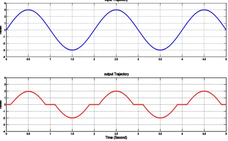
Figure 1 is the effect of deadzone on the output of a plant for a pure sinusoidal input trajectory. The majority of earlier investigations to this problem focus on the problem where the nonlinearity is located at the input of the plant as an actuator problem [1] [2]. In an actuator deadzone, the control effort is within the span of the nonlin-earity which makes it somewhat easier to reduce or eliminate its deleterious effects before it enters the dynamics of the system to be controlled. As a matter of fact, several papers present a two structure control schemes that can be designed to handle deadzone as well as other requirements for plant performance criteria [3]. On the other hand, output deadzone, which is physically inherent in some sensors that measure output signals of a plant, is a more complicated problem. The control effort has to eliminate the deleterious effect of the deadzone nonlinearity whilst going through the complicated dynamics of the plant. Therefore, whatever added control re-quirements enforced on the designer due to disturbances or noise affecting the plant, will further complicated the task. One of the earliest investigations of output nonlinearities such as deadzone was presented by [4]. Their proposed methodology was based on output matching control which involved the design of an adaptive dead-zone inverse used to reshape the input reference trajectory to negate the effect of the deaddead-zone. The parameters of the deadzone were adaptively estimated by designing an error function utilizing the output to observe plants states. The implementation was quiet complex in design and implemented in discrete time. In [5], an output feedback design was analysed for robustness and was developed using input to state stability (ISS) small gain tools. The combination of observer and controller design was proved to be essential when handling output nonlinearities. An adaptive compensation scheme without constructing a dead-zone inverse was presented in [6]. The proposed adaptive method requires only the information of bounds of the deadzone slopes and treats the time-varying input coefficient as a system uncertainty. The new control scheme ensures bounded-error trajectory tracking and assures the boundedness of all the signals in the adaptive closed loop. Tian Ping et al. utilized the integral-type Lyapunov function to design an adaptive compensation term for the upper bound of the residual and optimal approximation error as well as the dead-zone disturbance [7]. It was demonstrated that the closed- loop control system was semi-globally uniformly bounded. In [8], an inverse deadzone function was incorpo-rated in control system driven from a mathematical model of a deadzone in pneumatic servo valves. Tests were performed out using controllers with and without dead zone compensation to comparison validated the efficacy of the method. In [9], a somewhat earlier work was presented in discrete time which successfully achieved reduction
of the tracking error in plants with output deadzone nonlinearity while ensuring the global boundedness stability. The paper presented by Jing Zhoua et al. introduced a smooth approximation to the deadzone model which al-lowed them to employ back stepping technique [10]. In their approach, no knowledge was assumed of the un-certainty’s and the deadzone’s parameters. It is shown that the proposed controller not only can guarantee global stability, but also can achieve excellent transient performance. It is worthwhile to note that other non-classical control methods, such as fuzzy logic or neural network, have been presented by several researchers to reduce the effect of a deadzone nonlinearity [11]-[14]. For example, Wallace and Max used an adaptive fuzzy controller for nonlinear systems subject to dead-zone input. The boundedness of all closed-loop signals and the convergence properties of the tracking error are proven using Lyapunov stability theory and Barbalat’s lemma [15].
Motivated by the success in producing successful results in handling input deadzone, we present an extended method to reduce the errors caused by output deadzone nonlinearity. The proposed method relies on the premise that by pre-shaping the input trajectory to mimic an inverse form of the deadzone nonlinearity, the combined ef-fect will reduce if not completely eliminating the efef-fect of output deadzone.
In this paper, a new continuous time robust adaptive output deadzone inverse controller (RAODI) is used in conjunction with a conventional model reference adaptive control to counter the distortions cause by output deadzone. The ideal deadzone inverse controller is approximated by an infinitely differentiable implementation to insure asymptotic tracking and minimized error generation. The overall stability of the system under the pro-posed scheme will be proven analytically and demonstrated by simulation to a practical application. The struc-ture of the paper starts with a brief presentation of the dynamics of an output deadzone nonlinearity that defines various parameters and its effect on the output of a system are presented in Section 2. Meanwhile, the proposed control methodology is presented and its analytical proof using the Lyapunov argument is shown in Section 3. Consequently, an illustrative example of a model reference adaptive control scheme combined with the inverse control method is presented and followed by simulation results in Section 4.
2. The dynamics of Output Deadzone Nonlinearity
A common representation of a non-symmetrical deadzone nonlinearity, shown in Figure 1, can be described as follows
( )
(
)
(
)
, if
0, if
, if
r r
l r
l l
m x d x d
DZ y d x d
m x d x d
− >
= − < <
+ < −
(1)
where DZ y
( )
denotes the output of deadzone function, x t( )
the output of a plant, m is the slope of the lines,(
dr−dl)
is the width of the deadzone distance, and u t( )
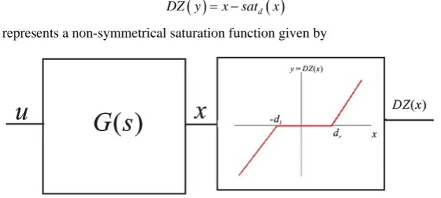
is the input of the plant block as shown in Figure 2. Although the width of the deadzone spacing is assumed not to be exactly known, an upper bounds on it is given byr l M
d −d ≤d (2)
where dM is a positive scalar. Output deadzone may also be written as
( )
d( )
DZ y = −x sat x (3)
[image:3.595.156.472.565.707.2]where satd
( )
u represents a non-symmetrical saturation function given by( )
, if , if , ifr r
d l r
l l
d x d
sat x x d x d
d x d
>
= < <
− < −
(4)
By defining a logical switching operator
1 if 0
0 otherwise r
x χ = >
(5)
1 if 0
0 otherwise l
x χ = <
(6)
Then, the dynamics of the non-symmetrical deadzone presented in (3) can be rewritten as follows
( ) ( )
( )
Tl l r r
y=DZ x =x t −χd −χ d =x t −d χ (7)
where x t
( )
is the. Meanwhile, thelogical indicators, χ=[
χ χr l]
can be implemented by utilizing the defini-tion of a sign funcdefini-tion given as( )
1 0sgn 1 0 d d d x x x > = − ≤
. (8) To obtain a smoothly differentiable implementation of (8), we replace it with a
( )
(
)
sgn xd ≈tanh ks⋅xd . (9) with ks >0 appropriately selected with high value for fast switching applications.
Hence, rewriting Equation (5) and Equation (6) as
(
)
1 tanh 2 s d r k xχ = + ⋅ (10)
(
)
(
)
1 tanh 1 . 2 s d l r k xχ = − ⋅ = −χ (11)
To proceed with the design of the compensator the following assumptions are required: (A1) The deadzone parameters dr >0 and − <dl 0 .
(A2) The deadzone parameters dr and dl are bounded as follows:
[
min, max]
l l l
d ∈ d d and dr∈
[
drmin,drmax]
.(A3) Without any loss of generality the slope of the deadzone m is positive and is set to 1.
Assumption (A1) and (A2) are the actual physical attributes of a real industrial deadzone and is adopted in [16]. Therefore, the saturation function given by (4) is physically bounded
( )
T .M
sat x = d χ ≤d (12)
3. Robust Adaptive Controller Design
Considering the following nonlinear systems with input deadzone nonlinearity described as
( )
{
( )
( )
}
( )
x Ax f x B u x
y DZ x
ψ
= + + +
=
(13)
where the matrices A and B are given by
0 1 0
0 0 1 0
0 0 0
= A 0 0 1 =
Meanwhile, the unmeasurable disturbances represented as ψ
( )
x and f x( )
are assumed to be bounded by a known pth order polynomial in the states [17]:( )
0 p k k k x x ψ ζ =≤
∑
(14a)( )
0 p k k kf x ζ x
=
≤
∑
. (14b)The desired reference model is given by
{
}
d d d
x = Ax +B Kx +r , (15)
where K∈R1×n and r is a reference signal. By reshaping the desired reference model in a way to produce a deadzone inversed version of it will reduce the effect of the deadzone. Tracking the reshaped copy of the refer-ence model will force the output of the deadzone nonlinearity to track the original desired referrefer-ence signal. The adaptive output deadzone inverse compensator can be deduced from (7) as
( )
* ˆ ˆ ˆT
d d d l l r r d
x =DI x =x +χd +χ d =x +d χ, (16)
where ˆT ˆ ˆ
r l
d = d d is the adaptively estimated values of the exact deadzone spacing * *
r l
d= d d . The
adap-tive inverse dynamics may be determined by differentiating (16) as follows
( ) ( ) ( ) ( )
* T
1
* * T T
2 1
* * T T T
3 * * T 0 ˆ ˆ ˆ
ˆ 2ˆ ˆ
ˆ
d d
d d d
d d d
n
n n k n k
nd d d
k
x x d
x x x d d
x x x d d d
n
x x x d
k
χ
χ χ
χ χ χ
χ − = = + = = + + = = + + + = = + ⋅ ⋅
∑
Consequently, we can utilize (15) to construct the inverse deadzone model reference as
( ) ( )
* *
0
ˆ .
n
k n k
T
d d d
k n
x Ax B K x d r
k χ − = = + ⋅ + ⋅ ⋅ +
∑
(17)
Hence, the states tracking error dynamics *
d
x= −x x may be written as follows
( )
( ) ( )0
ˆ ,
n
k n k
T d
k n
x Ax B u x K x d r
k
ψ χ −
= = + + − ⋅ − ⋅ ⋅ −
∑
(18)
where r is the desired reference signal. Equation (18) is written compactly as
( )
{
*}
.
d
x=Ax+B u+ψ x −Kx −r (19)
where dynamics of x*d are given by (17).
By defining the output tracking error
( )
t = −y xd an adaptive update law for T ˆd can be written as
( )
ˆ
d= −σ t χ (20)
Once again, by ensuring that the plant states x t
( )
tracking x t*d( )
will cause( )
(
*( )
)
(
(
( )
)
)
( )
d d d
y t =DZ x t =DZ DI x t =x + t (21)
( )
( )
*( )
( )
T( )
ˆTd d
y t y t x t d x t d
t = − = − χ− + χ
(22)
or simply written as
( )
Tt =d χ
. (23)
where T
d the deadzone parameters estimation error is
* T * ˆ , ˆ r r l l d d d d d − = −
(24)
Therefore, the deadzone effect noted by the term dTχ in (7) can be cancelled by simply ensuring that the system’s states vector x t
( )
track the inverse dynamics of the desired trajectory xd( )
t . To achieve proper tracking and global bounded stability of the overall system, we propose the following RAODI controller:( )
T ˆ T *d d
u t = −αB Px−βB Px+Kx +r (25)
where α>0, x= −x x*d, and P is the positive definite symmetric solution of the Algebraic Riccati equation (ARE). Moreover, the adaptation law for ˆβ is given by
T
ˆ Γ B Px , Γ 0.
β= > (26)
The properties of the controller (25) are stated in the following theorem:
Theorem. For the plant described by (13) with input deadzone (1), and the RAODI control law (25) along with the adaptive update laws (22) and (26) will ensure the closed-loop stability and boundedness of tracking error, hence reducing the effects of deadzone on the control law driving the system dynamics and ensures-bounded output tracking.
Proof. Using the following positive definite control Lyapunov function
1 1
T Γ 2 2
2 2
V x Px β σ d
− −
= + + (27)
Differentiating along the trajectories of the system and substituting for the closed loop dynamics given by (19) yields
( )
{
}
(
)
( )
{
}
(
)
T T 1 1
T *
T * 1 1
ˆ ˆ Γ ˆ ˆ Γ d d
V x Px x Px dd
Ax B u x Kx r Px
x P Ax B u x Kx r dd
ββ σ ψ
ψ ββ σ
− − − − = + + + = + + − − + + + − − + + (28)
Applying the robust controller given in (25) into (28) gives
( )
{
}
(
)
( )
{
}
(
)
T T TT T T 1 1
ˆ
ˆ
ˆ Γ ˆ
V Ax B B Px B Px x Px
x P Ax B B Px B Px x dd
α β ψ
α β ψ −ββ σ−
= + − − + + + − − + + + (29)
Collecting terms and simplifying
(
)
(
{
( )
}
)
(
)
(
{
( )
}
)
T T T T T 1 1
T T T T T 1 1
ˆ
ˆ ˆ
2 Γ
ˆ
ˆ ˆ
2 2 Γ
V x A P PA x x PB B Px B Px x dd
V x A P PA PBB P x x PB B Px x dd
α β ψ ββ σ
α β ψ ββ σ
− − − − = + + − − + + + = + − + − + + +
(30)
(
)
(
( )
)
T T T ˆ T T T 1 ˆ 1 ˆ
2 2 Γ
V=x A P+PA− αPBB P x−βB Pxx PB + x PB ψ x + −ββ σ+ −dd (31)
The first term can be simplified by solving the Algebraic Reccati Equation given by
T 2 T
which gives
( )
(
)
2
T ˆ T T 1 ˆ 1 Tˆ
2 Γ
V = −x Qx −β x PB + x PB ψ x + −ββ σ+ −d d (33)
Replacing the adaptation law (23) and replacing β β βˆ= + *
in (31) yields
(
)
2(
( )
)
2T * T 2 T T 1 Tˆ
V= −x Qx − β β+ x PB + x PB ψ x +β x PB +σ−d d (34)
( )
2
T * T T 1 Tˆ
2
V= −x Qx −β x PB + x PB ψ x +σ−d d (35)
Substituting the adaptive update law (7) dˆ= −σ
( )
t χ makes the fourth term in( )
( )
2
T * T 2 T T
V= −x Qx −β x PB + x PB ψ x −d t χ (36)
Utilizing Equation (23) for output tracking error
( )
t =dTχ.( )
( )
2
T * T 2 T T 2
V= −x Qx −β x PB + x PB ψ x − d χ (37)
Renders the last term negative. For the third term, we utilize the general inequality 2ab≤a2+b2 the third term in (37) can be bounded as
( )
T T 1
2x PB ψ x ≤ς x PB +ς− x (38)
Applying this bound to (37)
( )
(
)
2( )
21 * T T
min
V≤ − λ Q −ς γ− x −β x PB − d χ (39)
By choosing the degree of freedom ς satisfying the condition ς λmin
( )
Qγ
< and choosing β*
to be
greater than ς ensures all terms of V negative.
4. Illustrative Example & Simulations
To illustrate the efficacy of the proposed compensator a second order sinusoidal desired reference model is se-lected for tracking. Simulations of the system in (22) under the adaptive control law (23) and (24) have been performed for a sinusoidal reference trajectory given by xd
( )
t =3sin( )
πt represented by a second order model. The actual plant is also chosen to be a second order system simulating a rotational gear with deadzone resulting form the spacing between its meshing teeth.( )
( )
( )
1 2
m m m
l m m m
k k u t
DZ sat
θ θ θ
θ θ θ θ
+ + =
= = −
, (40)
where θ θm mT represent the driving motor angle and velocity respectively;
[
]
T 1 2
k k represent the viscous
friction and the electromotive force constant; and θl represents the output load angle. By defining the state vector
[
x x1 2]
T to represent θ θmm, then the system under investigation can be represented in space state form as( )
{
}
( )
( )
T
x Ax B k x u t
y DZ x x sat x
= + +
= = −
. (41)
where the matrices A and B along with the gain k are given by
1
2
0 1 0
, ,
0 0 1
k
A B k
k
= = =
Meanwhile, the desired reference model to be tracked at the output for the overall system may be rewritten as
( )
{
T 2}
3π sin
,
π
d d d
d
x Ax B k x t
y x
γ
= + −
=
(43)
where γ >0 used to insure the stability of the desired tracked model. In the case of meshing gears, the dead-zone spacing parameter can be easily predetermined and measured. The reference point is chosen to be at the center of the deadzone spacing. Hence, define d*=d*r = −dl*=1 with ˆd being the adaptation that estimate-sits value as given by Equation (20). Therefore, the adaptive deadzone inverse trajectory written as follows
( )
* ˆ
d d d
x =DI x =x +dχ
. (44) The proposed controller is given by
( )
T ˆ T *d d
u t = −αB Px−βB Px+Kx +r (45)
where the first term is the conventional PD-controller, the second term is the robust adaptive controller, and the third term is the adaptive deadzone inverse one.
T
ˆ Γ B Px , Γ 0.
β= > (46)
Meanwhile, the initial value of ˆd is set to be zero and no prior knowledge of its values is needed. The exact value of the simulated deadzone parameter is set to *
1
d = . For all other simulated parameters refer to Table 1.
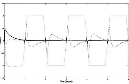
Figure 3 shows the output trajectory yo=θl for the system under RAODI control is presented and is com-pared to the trajectory tracking of the system under adaptive without the inverse (in dotted blue), and a PD-con- troller (dashed red). The system performance is shown with the black solid line while the performance of a regular PD controller is shown in dotted red line. Clearly, the output of the system under RAODI outperforms the system with a conventional PD controller. The deadzone spacing effect is practically eliminated and the tracking error is held to a small negligible amount.
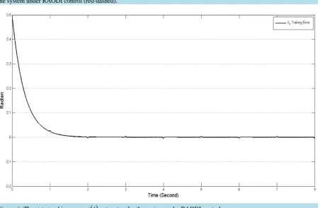
The improvement in reducing the effect of output deadzone on the output signal is demonstrated in Figure 4
where the error
(
yo−xd)
= −θ θl d is plotted in solid line as apposed to the same error for the system under a PD controller plotted in dotted red line. In addition, in Figure 4, the dashed blue line reflects the output track-ing error for the system without the use of inverse deadzone modifier. The error without the deadzone inverter is much larger than the improved performance due to RAODI controller.The system state x1=θm( )
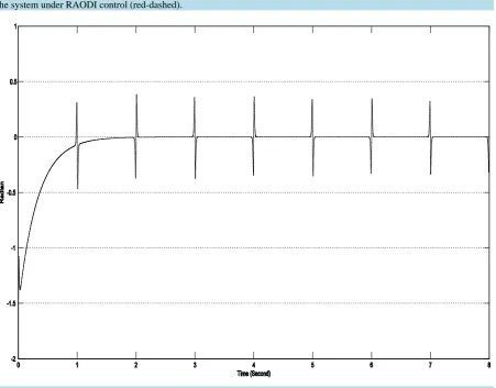
t tracking performance (solid) verses the deadzone inverted trajectory x1d =θd for the system under RAODI control is presented in Figure 5, with Figure 6 demonstrating the state tracking error ( )
t = −θ θl d for the system under the proposed control scheme. The second state x2=ω( )
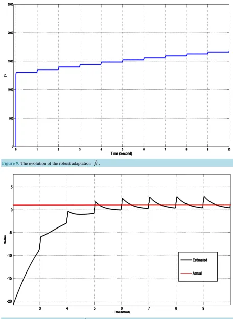
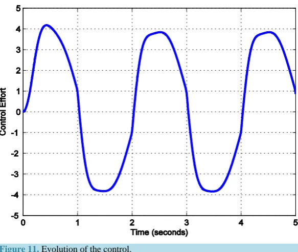
t tracking performance and its error 2= −ω ωd are presented in Figure 7 and Figure 8, respectively. In addition, Figure 9 and Figure 10 show the evolution of the adaptations βˆ and ˆd confirming their bounded stability. Meanwhile, the adaptive controller effort ud( )
t is shown in Figure 11.Table 1. Parameters utilized in the example.
Systems Physical Attributes
Parameter Value Unit
1 kp 40 Gain Constant
2 kv 13 Gain Constant
3 γ 100 Gain Constant
4 *
r
d 1.0 radian
5 *
l
d −1.0 radian
6 α 1.0 N.m/rad
7 Γ 100 Gains
8 J 1 V 2
s rad
−
⋅
Figure 3. The output trajectory yo (black-solid) for the system under RAODI control vs. the performance of an adaptive controller (blue-dotted), and a PD-controller (red-dashed).
[image:9.595.92.539.386.677.2]Figure 5. The system state x1=θ
( )
t tracking performance (solid) verses the deadzone inverted trajectory x1d =θd for [image:10.595.69.543.78.397.2]the system under RAODI control (red-dashed).
[image:10.595.90.543.413.707.2]Figure 7. The system state x2=ω
( )
t tracking performance (solid) verses the inverted deadzone trajectory x2d=ωd for [image:11.595.73.537.82.351.2]the system under RAODI control (red-dashed).
[image:11.595.90.542.354.707.2]Figure 9. The evolution of the robust adaptation ˆβ.
Figure 10. The evolution of the adaptation dˆ estimating the actual *
Figure 11. Evolution of the control.
5. Conclusion
In this paper, an adaptive inverse deadzone controller is compared with a robust adaptive controller for systems with output deadzone nonlinearity. Both controllers have been shown to effectively stabilize a second order sys-tem, and achieve bounded input bounded output (BIBO) tracking. The proposed deadzone inverse controller has greatly improved the performance of the system over the robust controller. The deadzone inverse controller was implemented in continuous time and was used to modify a desired model reference to mimic an inverse dead-zone trajectory. The RAODI is smoothly differentiable and can easily be combined with any of the advanced control methodologies. The stability of the closed-loop system has been proven by using Lyapunov arguments and simulations results confirm the efficacy of the control methodology.
Acknowledgements
This work is supported by the Public Authority for Applied Education and Training (PAAET) Kuwait grant number TS-14-03.
References
[1] Ahmad, N.J., Alnaser, M.J. and Alsharhan, W.E. (2013) Asymptotic Tracking of Systems with Non-Symmetrical Input Deadzone Nonlinearity. International Journal of Automation and Power Engineering, 2, 287-292.
[2] Tao, G. and Kokotovic, P. (1995) Discrete-Time Adaptive Control of Systems with Unknown Dead-Zones. Interna-tional Journal of Control, 61, 1-17. http://dx.doi.org/10.1080/00207179508921889
[3] Ahmad, N.J., Ebraheem, H.K., Alnaser, M.J. and Alostath, J.M. (2011) Adaptive Control of a DC Motor with Uncer-tain Deadzone Nonlinearity at the Input. 2011 Chinese Control and Decision Conference (CCDC), Mianyang, 23-25 May 2011, 4295-4299. http://dx.doi.org/10.1109/CCDC.2011.5968982
[4] Toa, G. and Kokotovic, P. (1996) Adaptive Control of Systems with Actuator and Sensor Nonlinearities. John Wiley & Sons, Inc., New York.
[5] Arcak, M. and Kokotovic, P.V. (2000) Robust Output Feedback Design Using a New Class of Nonlinear Observer. Proceedings of the 39th Conference on Decision and Control, Sydney, December 2000, 778-783.
[6] Ibrir, S., Xie, W.F. and Su, C.-Y. (2007) Adaptive Tracking of Nonlinear Systems with Non-Symmetric Dead-Zone Input. Automatica, 43, 522-530. http://dx.doi.org/10.1016/j.automatica.2006.09.022
http://dx.doi.org/10.1007/s11633-009-0124-5
[8] Andrighetto, P.L. and Bavaresco, D. (2008) Dead Zone Compensation in Pneumatic Servo Systems. ABCM Symposium Series in Mechatronics, 3, 501-509.
[9] Recker, D.A. and Kokotovic, P.V. (1993) Indirect Adaptive Nonlinear Control of Discrete-Time Systems Containing a Deadzone. Proceedings of the 32nd Conference on Decision and Control, San Antonio, 15-17 December 1993, 2647- 2653. http://dx.doi.org/10.1109/CDC.1993.325676
[10] Zhou, J., Er, M.J. and Wen, C.Y. (2005) Adaptive Control of Nonlinear Systems with Uncertain Dead-Zone Nonlinear-ity. 44th IEEE Conference on Decision and Control, and the European Control Conference, Seville, 12-15 December 2005, 797-801.
[11] Betancor-Martin, C.S., Montiel-Nelson, J.A. and Vega-Martinez, A. (2014) Deadzone Compensation in Motion Con-trol Systems Using Model Reference Direct Inverse ConCon-trol. 2014 IEEE 57th International Midwest Symposium on Circuits and Systems (MWSCAS), College Station, 3-6 August 2014, 165-168.
http://dx.doi.org/10.1109/MWSCAS.2014.6908378
[12] Jang, J.O., Chung, H.T. and Jeon, G.J. (2005) Saturation and Deadzone Compensation of Systems Using Neural Net-work and Fuzzy Logic. Proceedings of the 2005 American Control Conference, 3, 1715-1720.
http://dx.doi.org/10.1109/ACC.2005.1470215
[13] Chang, C.-Y., Hsu, K.-C., Chiang, K.-H. and Huang, G.-E. (2006) An Enhanced Adaptive Sliding Mode Fuzzy Control for Positioning and Anti-Swing Control of the Overhead Crane System. IEEE International Conference on Systems, Man and Cybernetics, 2, 992-997.
[14] Kong, X.Z. and Zang, F.Y. (2009) Study on the Intelligent Hybrid Control for Secondary Regulation Transmission System. IEEE International Conference on Automation and Logistics, Shenyang, 5-7 August 2009, 726-729.
http://dx.doi.org/10.1109/ICAL.2009.5262830
[15] Bessa, W.M. and Barrêto, R.S.S. (2010) Adaptive Fuzzy Sliding Mode Control of Uncertain Nonlinear Systems. Re-vista Controle & Automação, 21, 117-126.
[16] Lewis, F.L., Tim, W.K., Wang, L.-Z. and Li, Z.X. (1999) Deadzone Compensation in Motion Control System Using Adaptive Fuzzy Logic Control. IEEE Transactions on Control Systems Technology, 7, 731-742.
http://dx.doi.org/10.1109/87.799674
[17] Jain, S. and Khorrami, F. (1995) Robust Adaptive Control of a Class of Nonlinear Systems: State and Output Feedback. Proceeding of the 1995 American Control Conference, Seattle, June 1995, 1580-1584.