Spectral Gradient Algorithm Based on the Generalized Fiser Burmeister Function for Sparse Solutions of LCPS

(1)

http://dx.doi.org/10.4236/ojs.2015.56057

Spectral Gradient Algorithm Based on the

Generalized Fiser-Burmeister Function for

Sparse Solutions of LCPS

Chang Gao, Zhensheng Yu, Feiran Wang

College of Science, University of Shanghai for Science and Technology, Shanghai, China Email: [email protected]

Received 27 August 2015; accepted 20 October 2015; published 23 October 2015

This work is licensed under the Creative Commons Attribution International License (CC BY). http://creativecommons.org/licenses/by/4.0/

Abstract

This paper considers the computation of sparse solutions of the linear complementarity problems LCP(q, M). Mathematically, the underlying model is NP-hard in general. Thus an lp(0 < p < 1)

regu-larized minimization model is proposed for relaxation. We establish the equivalent unconstrained minimization reformation of the NCP-function. Based on the generalized Fiser-Burmeister func-tion, a sequential smoothing spectral gradient method is proposed to solve the equivalent prob-lem. Numerical results are given to show the efficiency of the proposed method.

Keywords

Linear Complementarity Problem, Sparse Solution, Spectral Gradient, Generalized Fischer-Burmeister

1. Introduction

Given a matrix M∈Rn n× and an n-dimensional vector q, the linear complementarity problem, denoted by LCP(q,

M), is to find a vector x∈Rn such that

(

)

T

0, 0, 0

x≥ Mx+ ≥q x Mx+q = .

The set of solutions to this problem is denoted by SOL M q

(

,

)

. Throughout the paper, we always suppose

(

,

)

(2)

solu-tion of the LCPs such as portfolio selecsolu-tion [3] [4] and bimatrix games [5] in real applications.

In this paper, we consider the sparse solutions of the LCP. We call x∈SOL q M

(

,

)

a sparse solution of LCP (q, M) if x is a solution of the following optimization problem

(

)

0

T

min

. 0, 0, 0

x

s t x≥ Mx+ ≥q x Mx+q = (1)

To be more precise, we seek a vector x∈Rn by solving the l0 norm minimization problem, where x₀

stands for the number of nonzero components of x. A solution of (1) is called the sparsest solution of the LCP. Recently, Meijuan Shang, Chao Zhang and Naihua Xiu design a sequential smoothing gradient method to solve the sparse solution of LCP [6]. We inspire by the model and use the spectral method based on the genera-lized Fischer-Burmeister function to solve our new model (3). The spectral method is proposed by Barzilai and Borwein [7] and further analyzed by Raydan [8] [9]. The advantage of this method is that it requires little com-putational work and greatly speeds up the convergence of gradient methods. Therefore, this technique has re-ceived successful applications in unconstrained and constrained optimizations [10]-[13].

In fact, the above minimization problem (1) is a sparse optimization with equilibrium constraints. From the problem of constraint conditions, as well as the non-smooth objective function, it is difficult to get solutions due to the equilibrium constraints to overcome the difficultly, and we use the NCP-functions to construct the penalty of violating the equilibrium constraints.

A function φ: R2 → R1 is called a NCP-function, if for any pair

( )

a b, T∈R2 ϕ

( )

a b, = ⇔ ≥0 a 0,b≥0,ab=0. A popular NCP-functions is the Fischer-Burmeister (FB), which is defined as

( ) (

)

2 2

,

FB a b a b a b

ϕ = + − +

The Fischer-Burmeister function has many interesting properties. However, it has limitations in dealing with monotone complementarity problems since it is too flat in the positive orthant, the region of main interest for a complementarity problem. In terms of the above disadvantage of the Fischer-Burmeister function, we consider the following generalized Fischer-Burmeister function [10].

( ) ( )

, ,

(

)

P a b a b _P a b

ϕ = − + (2)

where p is any fixed real number from P∈ +∞

(

1,

)

and

( )

, P

a b denotes the p-norm, i.e.

( )

, P P P

P

a b = a +b

In other words, in the function ϕP, we replace the 2-norm of

( )

a b, in the FB function ϕFB by a more

general p-norm of

( )

a b, . The function ϕP is still an NCP-function.

Define

( )

: n n P x R R

Φ → by

( )

(

)

( )

(

)

1, 1

,

P P

P n n

x F x x

x F x

ϕ

 

 

Φ =  

 

 



where F x

( )

=Mx+q with q∈Rn and M∈Rn n× . Obviously, x∈SOL M q

(

,

)

if and only if Φ_P

( )

x =0. By further employing the lpregularization term for seeking sparsity, we obtain the following unconstrained mi-nimization problem to approximate

( )

1

( )

2

min

2 n

p

P p

x R

f x x λ x

∈ = Φ + (3)

where λ∈

(

0,∞

)

is a given regularization parameter, and

1

n p p

i p

i

x x

=

∑

for any 0 < p < 1. We call (3) as lp regularized minimization problem.

(3)

( )

1

( )

2

P x P x

Ψ = Φ (4)

For any given P>1, the function ΨP

( )

x is shown to possess all favorable properties of the FB function;

we can see [8]. It plays an important part in our study throughout the paper. We observe in [14] [15] that P has a great influence on the numerical performance of certain descent-type methods; a larger P yields a better conver-gence rate, whereas a small P often gives a better global convergence.

The paper is organized as follows: In Section 2, we present absolute lower bounds for nonzero entries in local solution of (3). In section 3, we approximate the minimal zero norm solutions of the LCP. In section 4, we give a sequential smoothing spectral gradient method to solve the model. In Section 5, numerical results are given to demonstrate the effectiveness of the sequential smoothing spectral gradient method.

2. The l

p

Regularized Approximation

In this section, we consider the minimizers of (3). We study the relation between the original model (1) and the

lp regularized model (3), which indicates the regularized model is a good approximation. We use a threshold lower bound L [6] for nonzero entries in local minimizers and the choice of the lpminimization problem (3).

2.1. Relation between (3) and (1)

The following result is given in [6], which is essentially based on some results given by Chen Xiaojun [14]. Lemma 2.1. [6] for any fixed λ>0 the solution set of (3) is nonempty and bounded. Let x_λ be a solution of (3), and

{ }

λk be any positive sequence converging to 0. If SOL M q

(

,

)

≠φ, then

{ }

xλk has at least one ac-cumulation point, and any acac-cumulation point x of

{ }

k

x_λ is a solution of (3). That is, for any x∈SOL q M

(

,

)

satisfied

(

,

)

x∈SOL q M and x p_p ≤ x p_p.

2.2. Lower Bounds for Nonzero Entries in Solutions

In this section, we extend the above result to the lp norm regularization model (2) for approximating minimal l0 norm solutions of the LCP. We provide a threshold lower bound L > 0 for any local minimizer, and show that any nonzero entries of local minimizers must exceed L. Sincef x

( )

≥λ x p_p, the objective function f x

( )

is bound below and f x

( )

→ +∞ if x → ∞. Moreover, the set χ_p∗ of local minimizers of (3) is nonempty and bounded.

Lemma 2.2. [6] let x∗ be any local minimizer of (3) satisfying

( ) ( )

0

f x∗ ≤ f x for an arbitrarily given point 0

x . Set

(

)

( )

1 1

0 2 2 1

p

p L

M f x

λ −

 

 

= _ ₊ _

 

(5)

Then we have: for any i∈

{

1, 2,,n

}

,x_i∈ −

[

L L,

]

⇒x_i∗ =0. Moreover, the number of nonzero entries in x∗ is bounded.

( )

0

0 p

f x x

L λ

∗ _≤

Let us denote the first term of (3) by the function

( )

: n P x R R+

Ψ → . That is

( )

1

( )

2

P x P x

Ψ = Φ (6)

(4)

Lemma 2.3. [12] let ϕ_P:R2 →R1 be given by (3). Then, the following properties hold: 1) ϕP is a positive homogeneous and sub-additive NCP-function.

2) ϕP is strongly semismooth.

3) If

{

(

a bk, k

)

}

⊆ ×R R with ak → −∞, or bk → −∞, or ak → ∞, bk → ∞, then ϕP

(

a bk, k

)

→ ∞ when k→ ∞.

4) Given a point

( )

a b, ∈ ×R R, very element in the generalized gradient ∂ϕ_P

( )

a b, has the representation

(

ξ−1,ζ −1

)

, where

( )

1 1 sgn , P P P a a a b ξ − − ⋅

= and

( )

1 1 sgn , P P P b b a b ζ − − ⋅

= for

( ) ( )

a b, ≠ 0, 0

sgn(.) represents the sign function; ξ and ζ are real numbers that satisfy 1 1 ₁

P P

ξ − +ζ − ≤ _.

Theorem 2.1. The function ΨP

( )

x is continuously differentiable everywhere and the gradient of ΨP

( )

x

can be obtained by

( )

T

( )

P x Da x M Db x  P x

∇Ψ =_ + _Φ (7)

where Da

( )

x =diag

{

a xi

( )

}

and Db

( )

x =diag

{

b xi

( )

}

are diagonal matrices whose diagonal element is given by

( )

(

)

(

)

(

)

1 1 sgn

1 if , 0

, 1 otherwise P i i i P i i _i i _P i x x

x Mx q a x _x _Mx _q

ξ − −  _⋅  − + ≠  = +  − 

( )

( ) (

)

(

)

(

)

(

)

1 1 sgn

1 if , 0

, 1 otherwise P i i i P i i _i i _P i

x Mx q

x Mx q b x _x _Mx _q

ζ − −  _⋅ ₊  ₋ ₊ _≠  =  +   − 

where

(

ξ ζ,

)

is any vector satisfying 1 1 ₁

P P

ξ − +ζ − ≤ _.

3. Smoothing Method for l

p

Regularization

Most optimization algorithms are efficient only for convex and smooth problems. However, some algorithms for Non-smooth and non-convex optimization problems have been developed recently. Note that the term x p_p (0 <

p < 1) in (3) is neither convex nor Lipschitz continuous in n

R . Solving the non-convex, non-Lipschitz conti-nuous minimization problem is not easy. We use some approximation methods to surmount the non-Lipschitz continuity problem in solving (3).

Smoothing Counterpart for (3)

For µ∈

[

0,+∞

)

, let

( )

, ,

ln exp exp , .

t t

s t _t _t

t µ µ µ µ µ µ  >  =   ₊ ₋  _≤              (8)

It is clear to see that, for any t∈R,

( )

(

)

(5)

and s_µp

( )

t is continuously differentiable with

( )

(

)

( )

1 1 , exp exp

ln exp exp

exp exp

p

p p

p t sign t t

t t

s t _t _t

p t t t µ µ µ µ µ µ µ µ µ µ − −  _>       − − ′₌ _ _ _{ } _ _     ₊ ₋      _≤         _{ } _ _          _{ }₊ _₋ _  _{ } _ _ 

We can construct a smoothing approximation of (2) as

( )

2

( )

1 1 min 2 n n p P i

x R _i

fµ x x λ sµ x

∈ = Φ +

∑

₌ (9)

by noting that f_µ

( )

x is continuously differentiable, and

( )

0

limf_µ x f x

µ→ = since

( )

(

)

0≤ f_µ x −f x ≤λ µn ln 2 p (10) for any x∈Rn.

Let χp u, ∗

denote the set of local minimizers of (10). We have the similar results as in Lemmma 2.1 and 2.2, corresponding to the smoothing counterpart (10).

Theorem 3.1. Let

{ }

x_µ_k be a sequence of vectors being global minimizers of (10) with µ_k →0 as k→ ∞. Then, any accumulation point of

{ }

xµ_k is a global minimizer of (3).

Proof. Let x∗ be a global minimizer of (3) and x be an accumulation point of

{ }

xµk . We can deduce from (11) that

( )

k k

( )

k k

( ) ( )

(

kln 2

)

p

f xµ ≤ fµ xµ ≤ fµ x∗ ≤ f x∗ +λ µn

On the other hand, we have f x

( )

f x

( )

µk

∗ _≤

, and consequently

( )

_k

( )

(

_kln 2

)

p

f x∗ ≤ f x_µ ≤ f x∗ +λ µn

Which indicates x is a global minimizer of (3). Lemma 3.2. [6] for any µ >0, let xµ χp u,

∗_∈ ∗

be any local minimizer of (14) satisfying f x

( ) ( )

_µ∗ ≤ f x0

for an arbitrarily given initial points 0

x . Let L be defined in Lemma 2.2. Then, we have for any

{

1, 2, ,

}

,

( )

[

,

]

( )

i

i∈  n x_µ∗ ∈ −L L ⇒ x_µ∗ ≤µ

4. SS-SG Algorithm

We suggest a sequential Smoothing Spectral Gradient (SS-SG) Method to solve (3). With the SS-SG method, we need the Spectral Gradient method as the main step for decreasing the objective value. The smoothing me-thod is very easy to implement and efficient to deal with optimization; see [15].

We first introduce the spectral projected gradient method in [8] as follow. Algorithm 1. Smoothing Spectral Gradient Method

Step 0: Choose an initial point 0

n

x ∈R , and parameters σ∈

[

0, 0.5

]

, β ρ µ, , 0∈

[ ]

0,1 ,

30 10

η= . Let

1 1

α = , C1= fµk

( )

x1 , k=0.

Step1: Let gk = ∇fµk

( )

xk , dk = −αkgk

( )

αk ,

T 1 1 T 1 1 , k k k k k s s s y

α − −

− −

= where sk−1=xk −xk−1, yk−1 =gk−gk−1. If

0

k

g = , then stop.

Step 2: Compute the step size vk by the Armijo line search, where

{

}

0 1

max , , k

v = ρ ρ  satisfies

(

)

T

(

₁

)

k k k k k k k k k

f x +v d ≤C +σ αv g g µv −

(6)

Step 3: If ∇fµk

(

xk+1

)

≥nµk, then set µk+1=µk; otherwise, choose µk+1=βµk.

Algorithm 2. Sequential Smoothing Spectral Gradient Method Step 1: Find x by using the algorithm 1 to solve

( )

1

( )

2

min

2 n

p

P p

x R

f x x λ x

∈ = Φ +

Step 2: Compute

(

)

( )

1 1

0 2 2 1

p

p L

M f x

λ

λ −

 

 

= _ ₊ _

 

Use the lower bound L_λ to set the entries of x with small values to zeros and obtain the computed solution

x_λ with

( )

0 otherwise

i i

i

x x L

xλ λ

 ≥

=  

Step 3: Decrease the parameter λ and set x0:=xλ.

5. Numerical Experiments

In this section, we test some numerical experiments to demonstrate the effectiveness of our SG algorithm. In order to illustrating the effectiveness of the SS-SG algorithm we proposed, we introduce another algorithm of talking the LCPs. In [6], the authors designed a sequential smoothing (SSG) method to solve the lpregularized model and get a sparse solution of LCP(q, M). Numerical experiments show that our algorithm is more effective than (SSG) algorithm.

The program code was written in and run in MATLAB R2013 an environment. The parameters are chooses as 0.5

σ = , β =0.25 and µ0 =0.01. The maximum number of iterations in step 1 is set to be 2000. We end the SS-SG algorithm in Step 1, if fµk

( )

xk 105

−

∇ < and ₁₀ 4

k

µ _< −

, or it reaches the maximum number of itera-tions.

5.1. Test for LCPs with Positive Semidefinite Matrices

Example 1. We consider the LCP(q, M) with

0.4 0.3 0.1 0.4

0.3 0.3 0.3 0.3

0.1 0.3 0.7 0.1

M q

− −

   

   

= −_ − _ =_ _

 ₋  ₋ 

   

，

The solution set is SOL q M

(

,

) (

=

{

1, 0, 0

)

T+a

(

2, 3,1

)

T:a≥0

}

.

When a=0, the vector x∗=

(

1, 0, 0

)

T is the sparse solution of LCP(q, M). We choose P = 10, p = 0.1 in (3) for this small example, and use our SS-SG algorithm with the regularization parameter λ=0.01. We use the initial point x0=

(

3, 3,1

)

T, we get a minimal lp norm solution x=

(

1.000, 0, 0

)

and the distance

4

2.452 10

x∗−x = × − .

Example 2. We consider the LCP(q, M) with

5 1 1 4

1 1 1 , 0

1 1 2 2

M q

− −

   

   

= −_ _ =_ _

  ₋ 

   

The solution set is

(

) (

)

T

(

)

(

)

1 2 3 1 2 3

2 2

, , , : 1 , , 1 , 0 1

3 3

SOL q M = x x x x = + −a a x =a x = −a ≤ ≤a 

(7)

When a=0, the vector

T

1

2 2 , 0, 3 3

x∗=  _

  is the sparse solution of LCP(q, M). When a=1, the vector

(

)

2 1,1, 0

x∗= is the sparse solution of LCP(q, M). We choose the same parameters as Example 1. We use the in-itial point x0 =

(

2,1, 2

)

T, we get a minimal lp norm solution x=

(

0.667, 0, 0.667

)

and the distance

4 1 1.341 10

x∗−x = × − . We use the initial point x0 =

(

2, 2,1

)

T, we get a minimal lp norm solution

(

1.000,1.000, 0

)

x= and the distance x2 x 1.079 10 4

∗₋ ₌ _× −

.

These examples show that, given the proper initial point, our algorithm can effectively find an approximate sparse solution.

5.2. Test for LCPs with Z-Matrix [6]

Let us consider LCP(q, M) where

T

1 1 1

1

1 1 1

1 1

1 1 1

1 n

n n n M I ee n n n

n

n n n

 ₋ ₋ ₋ 

 

₋ ₋ ₋ 

 

= − =

 

− − −

 

 



   



and 1

1 1

1

n q n

n

 ₋ 

 

=

 

 



Here In is the identity matrix of order n and

(

)

T

1,1, ,1 n

e=  ∈R . Such a matrix M is widely used in statis-tics. It is clear that Mis a positive semidefinite Z-matrix. For any scalar a≥0, we know that the vector

1

x=ae+e is a solution to LCP(q, M), since it satisfies that

(

)

T 1

0, 0, 0

x≥ Mx+ =q Me + =q x Mx+q =

Among all the solutions, the vector x e1

(

1, 0, , 0

)

T

∗_{= =} _

is the unique sparsest solution. We test the SS-SG algorithm for different dimensions with n = 100, 300, 500, 1000, 1300, respectively. In this set of experiments, we set P=10,p=0.01, =0.01λ .The results are displayed in Table 1.

In Table 1, “ x−xˆ ” denotes the Euclidean distance between x and the true sparsest ˆx, and “time” de-notes the computational time in seconds. Form Table 1, we can see that the SS-SG algorithm is effective to find the sparse solution of LCPs.

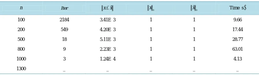
[image:7.595.194.438.249.350.2]

In order to test the effectiveness of the SS-SG algorithm, we compare with the SSG algorithm of talking the LCPs. In [10], the authors use the Fiser-Burmeister function established a lp (0 < p < 1) regularized minimization model and designed a SSG method to solve the LCPs. The results are displayed in Table 2, where “_” denotes the method is invalid. Although the sparsity x₀ is same and the recovered errors x−xˆ are pretty small, the average cpu time less than the SSG algorithm.

Table 1.SS-SG’s computation results on LCPs with Z-matrices.

n Iter x−xˆ x0 xˆ0 Time s( )

100 789 2.71E−3 1 1 2.25

200 452 5.22E−3 1 1 2.27

500 14 3.91E−4 1 1 4.02

800 11 4.21E−4 1 1 4.73

1000 3 1.64E−5 1 1 4.73

[image:7.595.89.536.573.720.2]

(8)

[image:8.595.88.537.99.231.2]

Table 2.SSG’s computation results on LCPs with Z-matrices.

n Iter x−xˆ x0 xˆ0 Time s( )

100 2184 3.41E−3 1 1 9.66

200 549 4.20E−3 1 1 17.44

500 18 5.11E−3 1 1 28.77

800 9 2.23E−3 1 1 63.01

1000 3 1.24E−4 1 1 4.13

1300 _ _ _ _ _

6. Conclusion

In this paper, we have studied a lp (0 < p < 1) model based on the generalized FB function defined as in (2) to find the sparsest solution of LCPs. Then, an lp normregularized and unconstrained minimization model is pro-posed for relaxation, and we use a sequential smoothing spectral gradient method to solve the model. Numerical results demonstrate that the method can efficiently solve this regularized model and gets a sparsest solution of LCP with high quality.

Acknowledgements

This work is supported by Innovation Programming of Shanghai Municipal Education Commission (No. 14YZ094).

References

[1] Facchinei, F. and Pang, J.S. (2003) Finite-Dimensional Variational Inequalities and Complementarity Problems. Sprin- ger Series in Operations Research, Vol. I & II, Springer, New York.

[2] Ferris, M.C., Mangasarian, O.L. and Pang, J.S. (2001) Complementarity: Applications, Algorithms and Extensions. Kluwer Academic Publishers, Dordrecht.

[3] Gao, J.D. (2013) Optimal Cardinality Constrained Portfolio Selection. Operations Research, 61, 745-761. http://dx.doi.org/10.1287/opre.2013.1170

[4] Xie, J., He, S. and Zhang, S. (2008) Randomized Portfolio Selection with Constraints. Pacific Journal of Optimization,

4, 87-112.

[5] Cottle, R.W., Pang, J.S. and Stone, R.E. (1992) The Linear Complementarity Problem. Academic Press, Boston. [6] Shang, M.J., Zhang, C. and Xiu, N.H. (2014) Minimal Zero Norm Solutions of Linear Complementarity Problems.

Journal of Optimization Theory and Applications, 163, 795-814. http://dx.doi.org/10.1007/s10957-014-0549-z [7] Barzilai, J. and Borwein, J.M. (1988) Two Point Step Size Gradient Method. IMA Journal of Numerical Analysis, 8,

174-184. http://dx.doi.org/10.1093/imanum/8.1.141

[8] Raydan, M. (1997) The Barzilai-Borwein Gradient Method for the Large Scale Unconstrained Optimization Problem.

SIAM Journal on Optimization, 7, 26-33. http://dx.doi.org/10.1137/S1052623494266365

[9] Raydan, M. (1993) On the Barzilai and Borwein Choice of Step Length for the Gradient Method. IMA Journal of Nu-merical Analysis, 13, 321-326. http://dx.doi.org/10.1093/imanum/13.3.321

[10] Chen, J.-S. and Pan, S.-H. (2010) A Neural Network Based on the Generalized Fischer-Burmeister Function Fornonli-near Complementarity Problem. Information Sciences, 180, 697-711.http://dx.doi.org/10.1016/j.ins.2009.11.014 [11] Chen, J.-S. and Pan, S.-H. (2008) A Family of NCP Functions and a Descent Method for the Nonlinear

Complementar-ity Problem. Computation Optimization and Application, 40, 389-404. http://dx.doi.org/10.1007/s10589-007-9086-0 [12] Chen, J.-S. and Pan, S.-H. (2008) A Regularization Semismooth Newton Method Based on the Generalized Fischer-

Burmeister Function for P0-NCPs. Journal of Computation and Applied Mathematics, 220, 464-479.

http://dx.doi.org/10.1016/j.cam.2007.08.020

(9)

[14] Chen, X.J., Xu, F. and Ye, Y. (2010) Lower Bound Theory of Nonzero Entries in Solutions of l2-lpMinimiization.

SIAM: SIAM Journal on Scientific Computing, 32, 2832-2852. http://dx.doi.org/10.1137/090761471

[15] Chen, X. and Xiang, S. (2011) Implicit Solution Function of P0 and Z Matrix Linear Complementarity Constrains.