Behavioural patterns in social networks

(1)

BIROn - Birkbeck Institutional Research Online

Conte, A. and Di Cagno, D. and Sciubba, Emanuela (2015) Behavioural

patterns in social networks. Economic Inquiry 53 (2), pp. 1331-1349. ISSN

0095-2583.

Downloaded from:

Usage Guidelines:

Please refer to usage guidelines at or alternatively

(2)

Behavioural Patterns in Social Networks

Anna Contea,b, Daniela T. Di Cagnoc, Emanuela Sciubbad

a_{Max Planck Institute of Economics, Kahlaische Str. 10, 07745 Jena, Germany} b

University of Westminster, EQM Department, 35 Marylebone Road, NW1 5LS London, UK

c_{LUISS University, Viale Romania 32, 00198 Rome, Italy} d

Birkbeck, University of London, Malet Street, Bloomsbury, WC1E 7HX London, UK

Abstract

In this paper, we focus on the analysis of individual decision making for the formation of

social networks, using experimentally generated data. We analyse the determinants of the

individual demand for links under the assumption of agents’ static expectations and

iden-tify patterns of behaviour which correspond to three specific objectives: players propose

links so to maximise expected profits (myopic best response strategy); players attempt

to establish the largest number of direct links (reciprocator strategy); players maximise

expected profits per direct link (opportunistic strategy). These strategies explain

approx-imately 74% of the observed choices. We demonstrate that they are deliberately adopted

and, by means of a finite mixture model, well identified and separated in our sample.

JEL classification: C33; C35; C90; D85

(3)

1 Introduction

Individual strategies for network formation can be extremely complex. The main reason for

this is that a network differs from a series of bilateral relationships because of the value

of indirect connections: any two economic agents who have to decide whether to establish

a social tie take into account not only their own characteristics and the characteristics of

the prospective partner but also their (and the prospective partner’s) position in the social

network.

The theoretical literature on endogenous network formation stems from the seminal

con-tributions by Myerson (1991), Jackson and Wolinsky (1996) and Bala and Goyal (2000).

These papers take a game-theoretic approach to the formation of social ties where the main

idea is that players earn benefits from being connected both directly and indirectly to other

players and bear costs for maintaining direct links. Predicted outcomes are typically not

unique. Even for those cases where the stable network architecture is unique (for example

the star network in information communication models `a la Bala and Goyal or Jackson and

Wolinsky), the coordination problem of which agent occupies which position in the network

still remains.

In presence of multiplicity of equilibria and coordination problems, it is hardly surprising

that most experimental contributions on this topic have highlighted the difficulty in obtaining

convergence to a stable network architecture as predicted by the theory.1

Since the observed network structures are ultimately the outcome of individual linking

decisions, one possible approach to overcome this difficulty is to investigate the process of

network formation in order to identify patterns of individual behavior that can be resumed

in prevailing linking strategies.

With this aim, we use data of a computerised experiment of network formation, where all

connections are beneficial and only direct links are costly. The network formation protocol

1_{More in detail: while convergence may be more easily achieved in experimental settings where the stable}

(4)

that we adopt, unlike the one used by most of the experimental literature that has focused on

convergence, requires that links are not unilateral, but have to be mutually agreed in order to

form. In particular, players simultaneously submit link proposals, but a connection is made

only when both players involved agree. We collect data from 9 groups of 6 participants each

and a minimum of 15 rounds of network formation.

In this paper, we estimate a system of equations that model each player’s decision on the

opportunity to propose a link to any of her prospective partners in each round of the game.

This approach allows us to take into account the fact that from a player’s perspective the

decision to propose a link to one of her opponents is not separate from the decision to propose

or not a link to another opponent; therefore, decisions made by the player in each round of

the game are the result of a joint valuation.

Relying on the results of such an analysis, we attempt to categorise players’ systematic

behaviour into a set of possible strategies adopted by the experimental subjects in our network

formation game.

An obvious departing point to interpret these results is to consider myopic best response

behavior, where players propose links so to maximise current profits while taking other players’

link proposals as given. This is a useful benchmark because most of the theoretical literature

on strategic network formation makes the assumption that agents behave according to myopic

best response and focuses on Nash Equilibrium (and refinements of Nash Equilibrium) as the

appropriate solution concept for the network formation game.

Given the payoff structure of the network formation game which we consider here, myopic

best response requires subjects to propose (direct) links to all those that in the current network

are not already reached through indirect connections. It is always advantageous, for example,

to propose a link to an isolated node. On the other hand, redundant links (i.e. links to those

nodes that are reached also through indirect connections) should be deleted. Also, given that

links are only established if they are requested by both players involved, proposing a link to

a player from which a link proposal has not been received is always a matter of indifference.

When all agents play according to myopic best response, the emerging network architecture

(5)

contains also trivial network structures such as the empty network. The empty network is

a Nash network (i.e. a network structure induced by agents who play myopic best response)

because links have to be mutually agreed in order to form, hence not proposing while not being

proposed is always a best response. To get more interesting and more focused predictions,

the theoretical literature on network formation has proposed pairwise stable networks as a

suitable refinement of Nash networks. A network is pairwise stable when it is: (1) Nash,

and (2) such that all mutually profitable links have been activated. Pairwise stable networks

are both minimal and connected, in that all nodes are connected and through the smallest

number of links.

By accepting pairwise stability as the appropriate solution concept for the network

for-mation game, most of the experimental literature has focused on whether convergence to a

minimally connected network structure, such as the star, or the chain, obtains in the lab.

Minimally connected graphs are often reached in our experimental groups (21 out of 157,

which correspond to a 13% of the total network configurations) but are typically unstable.

Convergence to a minimally connected network is only observed in one out of the nine

ex-perimental groups (group 7), where the same minimally connected graph is reached and then

kept for four rounds until the end of the session. Mostly we observed connected graphs which

are not minimally connected (68 out of 157, which correspond to a 43% of the total network

configurations).

We went on to speculate which behaviour, other than myopic best response, may concur

in explaining the observed network architectures.

We start our analysis with a preliminary investigation of the determinants of individual

linking decisions (see Section 3). In accordance with myopic best response behavior, we find

that subjects are less likely to propose links to those that can already be reached through

in-direct connections. Moreover we find a tendency to reciprocate link proposals and a tendency

to propose links to those who have the largest number of connections which is not necessarily

in accordance with best response behaviour.

This observation motivates the two residual patterns of behaviour we consider in this

(6)

“opportunistic” strategies.

A subject who follows the “reciprocator” strategy makes link proposals to all those from

whom link proposals have been received. Other than maximising expected profits, a

recip-rocator aims to establish the largest number of direct links. As for best response behavior,

reciprocators will not leave profitable linking opportunities unexploited; however, unlike best

response behavior, they may keep redundant links. Reciprocators maximise revenues, rather

than profits, and do not care about minimising the cost through which a high connectivity is

obtained.

A subject who follows the “opportunistic” strategy only activates those links (among the

ones which are feasible, in that proposals have been received by the other party involved)

which are most profitable because bring the largest number of indirect connections. While

this behavior may seem closer to profit maximisation because both costs and revenues of link

formation are taken into account, it differs from myopic best response in that profitable link

opportunities may be neglected (and at the same time there is no guarantee that redundant

links will be avoided).

We then go on to verify from our data whether the identified strategies are well represented.

Finally, in order to discriminate among these three types of systematic behaviour, we estimate

a mixture model to establish if these strategies are well identified and separated in our sample.

We find that it is safe to assume that each subject in our sample belongs to one type, with

mixing proportions approximately equal to 45%, 30% and 25% for best response, reciprocator

and opportunistic types, respectively.

We notice that the payoffs achieved by the three types are not too dissimilar, with

oppor-tunists earning marginally less than myopic best responders and reciprocators.

Finally, we note that the propensity to adopt a certain strategy is group-driven, with

subjects being more likely to best respond, to reciprocate and to behave opportunistically

when others in the same group also do.

The fact that behavioural patterns (similar to, but) other than myopic best response

be-haviour are significantly represented in the population may explain why the observed network

(7)

My-opic best response agents will always tend to include isolated nodes and delete redundant

links, whereby pushing the network architecture to a minimally connected graph. If at any

stage two reciprocators link up, then that link will not be deleted even when it is redundant,

which may result in stable network configurations which are not minimal. Finally, the

pres-ence of opportunists along with myopic best response agents and reciprocators may favour,

when prevalent, the emergence of asymmetric network configuration such as the star, over

alternative architectures. For example, when there is a single myopic best response agent

and everyone else is an opportunist, the network converges to a star (where the myopic best

response agent is the hub). Hence the exact mix of strategies represented in the population

can help us predict which network architecture will emerge in equilibrium.

The paper proceeds as follows. Section 2 describes the experimental design: the model

and the experimental procedure. Section 3 presents and discusses the results of the model

of link proposals described in Appendix A. Section 4 shows the characteristics of the three

behavioural types that emerged from the analysis in Section 3. Section 5 analyses the data

in the light of these three behavioural types. Section 6 develops the mixture model, and

Section 7 concludes. The econometric model of link proposals is explained in Appendix A.

The instructions (in their English translation) can be found in Appendix B.2

2 The Experimental Design

2.1 The Model

We model network formation as a non-cooperative simultaneous move game. As in Myerson

(1991), we assume that players’ strategies are vectors of intended links and that links are

only formed when they are mutually agreed, i.e. desired by both parties involved. There

are positive network externalities in that both direct and indirect connections are beneficial;

however direct links are costly.

Consider a set N of n ≥ 3 players, indexed by i = 1,2, . . . , n. Each player i submits a

2

(8)

vector of intended links:

si = (si1, si2, . . . , sin)

An intended link is sij ={−1,1} wheresij = 1 means that playeriintends to link to player

j while sij = −1 means that playeri does not intend to link to player j. A link between i

and j is formed if and only if sij = sji = 1. We denote the formed link by gij = gji = 1,

while we represent the fact that there is no mutually agreed link betweeniand j by setting

gij =gji= 0. A strategy profile for all players

s= (s1, s2, . . . , sn)

induces an (undirected) network of links g = {gij}_i,j_∈_N, where players are nodes and links

are the edges between them. We say thatiandj are connected in the graphg if there exists a path of adjoining nodesk1, k2, . . . , km such that gik1 =gk1k2 =· · ·=gkm−1km =gkmj = 1.

Denote by nd_i the number of direct neighbours of player i, and by ni the number of her

direct and indirect connections. More in detail, denote bynd_i the number of elements of the setN_id={j|gij = 1} and byni the number of elements of the set Ni ={j |there is a path

ingfromitoj}.Notice that ifiand jare directly linked, then there is a path between them (of length 1): hence necessarilyni ≥ndi. Playeri’s payoff, given her position in the network

g, is assumed to be equal to:

πi(g) =b×ni−c×ndi,

wherebandcrepresent, respectively, the unitary benefit from (direct and indirect) connections

and the unitary cost of direct links and are such thatb > c >0.

In this game, players simultaneously announce all the links they wish to form and the

resulting network is formed by the mutually announced links. “This game is simple and

intuitive. But, given that link creation requires the mutual consent of the two involved

parties, a coordination problem arises. As such the game displays a multiplicity of Nash

equilibria, and very different network geometries can arise endogenously.” (Calv´o-Armengol

(9)

stable) networks as a refinement of Nash networks. Pairwise equilibrium networks are not

only robust to unilateral deviations (all redundant links are deleted), but also to bilateral

deviations which may make any two players coordinate on the formation of a new link so that

no mutually beneficial links are left inactive.3

Formally:

Definition: A network g is a pairwise equilibrium network if the following conditions hold:

1. there is a Nash equilibrium strategy profile (s∗_i, s∗₋_i) that induces g;

2. for gij = 0,if πi(g+gij)−πi(g)>0 then πj(g+gji)−πj(g)<0

Goyal and Joshi (2006) show that all network architecture which are induced by a Nash

equilibrium strategy profile (Nash networks) are minimal. A minimal graph is such that there

is at most one path connecting any two agents: there are no redundant links. The intuition

why this has to hold is that if there are redundant links, then there are agents who can be

reached both directly and indirectly. Agents could obtain higher payoffs by deleting their

(costly) direct links to all those nodes that they are able to reach indirectly through others.

As long as b > c >0, all pairwise equilibrium networks are both minimal and connected (or minimally connected), i.e. there is one and only one path connecting any two agents.4

The intuition behind this is that if there is any isolated node, given that the benefit from an

extra connection is higher than the cost of a direct link (b > c), then there are incentives for a new link to be formed between the isolated player and at least another node in the graph.

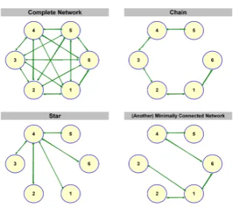
Examples of network architectures are in Figure 1. The complete network, where every

node is directly connected to every other, is an example of connected graph. The complete

network is clearly not minimal as there are many redundant links. Examples of minimally

connected graphs are the star and the chain.

3_{See Goyal and Joshi (2006), Calv´}_{o-Armengol (2004) and Bloch and Jackson (2006) for applications of}

pairwise equilibrium networks.

4

(10)

[image:10.595.216.387.103.256.2]

Figure 1: Examples of network architectures.

2.2 The Experimental Procedure

The experimental sessions were conducted in spring 2006 and 2008 at CESARE, LUISS

Uni-versity in Rome with a total of 54 participants.5 Subjects were first-year Economics students.

Each subject participated in only one session and none had previously taken part in a similar

experiment. Each experimental sessions was made of 2/3 groups of 6 participants each,

play-ing together in a network formation game. Each experimental session lasted between 30 and

45 minutes. Subjects’ total earnings were determined by the sum of the profits in each round

and were paid using a conversion rate of 100 points per euro. They earned approximately

e32 on average, on top of a e5 participation fee.

While in the sessions that were conducted in spring 2006 we implemented two alternative

treatments, with different cost parameters, in the present paper we only analyse data from

one of the two treatments, for which detailed parameters are given in the table below:6

Participants Initial Endowment Cost Benefit

Groups 1 - 9 6 500 90 100

5_{Here we re-analyse the data from Treatment 1 in Di Cagno and Sciubba (2008), plus some newly collected}

data. More in detail, of the 9 groups considered here, 7 coincide with those analysed for Treatment 1 in Di Cagno and Sciubba (2008) and were collected in spring 2006. In spring 2008 we collected data for 2 additional groups under the same experimental protocol used for the 2006 data. More independent observations than we had in 2006 were required for the econometric analysis conducted in this paper.

6

(11)

[image:11.595.189.413.106.264.2]

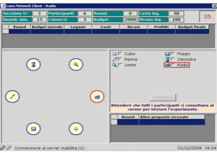
Figure 2: The initial screen

All relevant parameters were equal across participants and displayed on the screen at all

time throughout the experiment.

At the beginning of each session subjects were told the rules of conduct and provided with

detailed written instructions, which were read aloud by the experimenters.

Sessions consisted of a minimum of 15 rounds, with a random stopping rule determining

the end of the experiment.7 In each round, subjects were asked to submit (anonymously and

independently) a vector of intended links. The initial screen for each participant is shown in

Figure 2.

Participants were represented on the screen by different symbols which we considered

neutral in that they did not provide subjects with any particular clue when deciding to

establish a link with another player in the group.8 _{Subjects did not know their symbol}

(or the other participants’ symbols) in advance and could identify themselves on the screen

because their symbol was circled in red. In order to guarantee not only individual but also

group anonymity, participants were invited to the lab in groups of eighteen, with three groups

7

At the end of round 15 (and of each additional round after that), a lottery administered by the computer decided if an additional round had to be played. The probability of new rounds was fixed at 50%. The lottery was visualised on participants’ screens by two flashing buttons, one red (with a NO sign) and one green (with a YES sign).

8_{In this setting we wanted to avoid any salient coordination device that induces coordination in a particular}

(12)

[image:12.595.190.412.107.264.2]

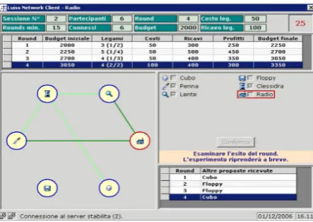
Figure 3: An example of the participants’ screen at the end of a round

being matched at the same time. Participants were not told in which of the three groups of

six they were playing, nor could they identify the group from their seating.9

The screen also displayed the relevant parameters for the session at play. After all

sub-jects had confirmed their choice of network partners, the computer checked which links were

mutually desired and activated them. At the end of each round, profits were computed and

displayed on the screen. Great care was taken in making sure that all available information

was provided to the experimental subjects in a user-friendly way. For this reason the graphical

interface was designed such that actual links were visualised on the screen as a graph rather

than a list of activated ties or as a matrix of−1/1 connections.

As an example, Figure 3 shows the players’ screen at the end of round number 4. It

displays the graph of all active links, total revenues, costs and profits in the round. It also

provides information on past unmatched proposals: at the end of a round each subject was

informed of those players who proposed a link to them but to whom they did not reciprocate.

At any time during the experiment, subjects had access to a great deal of information on past

history: by clicking on the bar corresponding to each round, they were able to visualise the

graph of active links and the profits obtained in that round.

9_{While we always invited 18 subjects to the lab, in a few occasions we could only collect data for 2 groups}

(13)

3 The Model of Link Proposals

In this section, we analyse and discuss the determinants of link proposals. In doing so, we

make the assumption of players having static expectations; that is, we assume that each player

expects her opponents to make exactly the same choices in roundtas in roundt−1. This is in line with most of the theoretical literature on network formation; also, to a certain extent,

such expectations are induced by the design of the experiment itself: the networks that result

from choices in previous rounds are portrayed on the computer screen together with all the

relevant information and made accessible throughout the game.10

Using the system of equations described in Appendix A, we estimate the probability of

each subject i proposing a link to any of her prospective partners j, with j = 1, . . . ,5, as a function of the position of i and j in the network reached in the previous round, which is

represented graphically on the subject’s screen. More in detail, we estimate the probability

of subjects proposing a link as a function of a number of variables that can be classified into

four categories: the characteristics of the relationship proposer-recipient, which, in particular,

include the lagged dependent variable; the characteristics of the prospective partner; the

characteristics of the proposer herself; the characteristics of the network of links observed in

the previous round. We also control for experience.

This exercise is meant as a preliminary analysis aiming to verify whether there is

system-atic behaviour in players’ link proposals that might be ascribed to the application of certain

strategies and, consequently, to identify and to study such strategies.

3.1 Estimation Results

The estimation results of the 5-equation multivariate dynamic probit model derived in

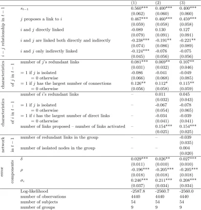
Ap-pendix A are reported in Table 1.11

The relationship between i and her opponent, j, in t−1 is described by the first five

10

In contrast to what we assume here, see Carrillo and Gaduh (2011) and Mantovani et al. (2011) for experimental evidence on farsighted behaviour in network formation.

11_{We have estimated several specifications of the model of link proposals, using many combinations of}

(14)

regressors. Let us start observing that the coefficient on the lagged dependent variable,st−1,

is positive and strongly significant, which conveys the idea that subjects tend to build on what

they did in the previous round. Given the strong statistical significance of the coefficient on

‘j proposes a link toi’, it seems more likely that a link is proposed if the recipient demanded a link to the proposer in the previous round. This could denote both a behavioural tendency

to reciprocate and a rational response. In fact, under the assumption of static expectations

(i.e. if players expect their opponents to make the same choices in roundtas they did in round

t−1), given that links have to be mutually agreed, a link can only be established by proposing a link to proposers in the previous round. The fact of i and j being linked directly plays no role here, in that the variable ‘iand j directly linked’, which is an interaction term between ‘st−1’ and ‘j proposes a link toi’, shows not to be statistically significant in any specification.

Anyhow, there is some evidence on the tendency to cut redundant links through the negative

and statistically significant coefficient on the variable ‘i and j are linked both directly and indirectly’. The attitude not to form redundant links is corroborated by the negativity and

statistical significance of the coefficient on the variable ‘i and j only indirectly linked’, even if not in terms of all the specifications of the model. Therefore, the probability of proposing

a link seems to diminish if i and j were previously linked both directly and indirectly and if they were already linked but only indirectly.

This first set of findings essentially describes the behaviour of a myopic best responder, as

delineated in the Introduction, but there is something more. The coefficient on the variable ‘j

proposes a link toiint−1’ showed to be positive and strongly significant in any specification. This makes us conclude that, other than a tendency to best respond to the previously formed

network, there might be subjects who simply reciprocate demanded links.

In our opinion, another possible motive of link formation can be extrapolated from the

results regarding the probability of iproposing a link toj as a function ofj’s characteristics, which seem to portray the figure of a player acting in a rather opportunistic way. In effect,

the estimation results disclose that players tend to propose links to those who have the largest

(15)

(1) (2) (3) i − j relationship in t −

1 st−1 0.560*** 0.400*** 0.400***

(0.062) (0.060) (0.060) jproposes a link toi 0.467*** 0.460*** 0.459***

(0.059) (0.058) (0.058) iandjdirectly linked -0.089 0.130 0.127

(0.079) (0.091) (0.091) iandjare linked both directly and indirectly -0.238*** -0.191** -0.221**

(0.074) (0.086) (0.089) iandjonly indirectly linked -0.124*** -0.076 -0.075

(0.045) (0.056) (0.056)

characteristics of

j

in

t

−

1 number ofj’s redundant links 0.081*** 0.069** 0.107** (0.031) (0.032) (0.046) = 1 ifjis isolated -0.086 -0.041 -0.049

= 0 otherwise (0.066) (0.068) (0.085)

= 1 ifjhas the largest number of connections 0.126** 0.112* 0.115**

= 0 otherwise (0.056) (0.058) (0.059)

characteristics of i in t − 1

number ofi’s redundant links – 0.011 0.045 (0.032) (0.043)

= 1 ifjis isolated – -0.067 -0.078

= 0 otherwise (0.054) (0.065)

= 1 ifihas the largest number of direct links – -0.034 -0.039

= 0 otherwise (0.041) (0.041)

number of links proposed – number of links activated – 0.154*** 0.154*** (0.025) (0.025) net w ork in t −

1 number of redundant links in the group – – -0.039 (0.035) number of isolated nodes in the group – – 0.004

(0.020)

error

comp

on

en

ts δ 0.029***_(0.011) 0.026**_(0.010) 0.027***_(0.010)

ρ -0.196*** -0.205*** -0.205***

(0.018) (0.018) (0.018)

σi 0.246*** 0.211*** 0.208***

(0.037) (0.034) (0.034)

Log-likelihood -2587.8 -2560.7 -2560.0

number of observations 4440 4440 4440

number of subjects 54 54 54

[image:15.595.97.510.111.541.2]

number of groups 9 9 9

Table 1: Estimation results of three specifications of the model of link proposals detailed in Appendix A. The coefficients on the group fixed effects,λg, are omitted.

∗ ∗ ∗,∗∗and∗indicate ap-value<0.01,<0.05 and<0.10, respectively.

the opponent’s redundant links – an indicator of high connectivity.12 If a player is instead

isolated – that is, she has no connection of any sort – the other players do not seem to be

willing to include her.

Among the variables that describeiin the previous round, we find strong evidence of the fact that the propensity to demand a link increases only if the breakdown rate in the previous

12_{Here again, the evidence is not extremely robust, making us suspect that only part of the population may}

(16)

round – measured as the difference between the number of links proposed and the number of

links activated – increases.13

We also estimate the propensity to propose a link as a function of the characteristics of the

network of links that emerged in the previous round. Despite the large number of variables

representing the network structure tested, none of them seem to play a significant role in

subjects’ decision. An example is reported in the third column of Table 1. It shows that

neither the coefficient on the number of redundant links nor that on the number of isolated

nodes in the group are statistically significant. We therefore conclude that players did not

take into account the global structure of the network established in the previous round when

expressing their willingness to demand a link and choosing the receiver of that proposal.

Table 1 also shows that the correlation coefficient ρ is precisely estimated to be about

−0.20. It is also significantly different from zero and negative, as expected. This indirectly supports our reasons for dealing with individual link proposals as being jointly determined.

The considerable magnitude of the standard deviation of the individual-specific propensity

to demand links, σα, puts into evidence the heterogeneity of the population. Finally, the

coefficientδis estimated to be positive and significantly different from zero, so indicating that the noise diminishes, the higher the level of experience that players accumulate by playing

the network game for several rounds.

Given these results, in what follows we study the distribution of three basic patterns of

behaviour adopted by the experimental subjects in our sample:

• players who reciprocate to those who demanded a link in the previous round unless they

can be reached otherwise through indirect connections (under the assumption of static

expectations, this behaviour corresponds, in fact, to profit maximisation);

• players who act by simply reciprocating link proposals from the previous round;

• players who try to reach the largest number of nodes by reciprocating to those who

exhibit a high connectivity.

13_{In our setting, reaching a node directly when it is already reached indirectly is always more beneficial than}

(17)

As stated earlier, this exercise was meant to search for the leading motives of individual

linking decisions, which essentially correspond to the maximisation of: expected profits; direct

links; and expected profits per link. In what follows, we will delineate the behavioural rules

which define these types of player, and we will try to establish whether these patterns of

behaviour are deliberately and systematically adopted by the subjects in our sample and, if

so, in which proportion of the observed sample the different types are represented.

4 Strategies of Link Formation

In each round of link formation, individuals have 32 available strategies. For each player, a

strategy is given by a 5-dimensional vector of 0s and 1s. For example, a possible strategy of

player 1 is to propose a link to each of the other 5 players in the game:

(1,1,1,1,1)

Strategy (0,0,0,0,0) corresponds to the choice of not proposing a link to any of the other players, while (1,1,0,0,0) corresponds to the choice of proposing to the first two players (other than player 1) and not the other ones, and so forth.

Under the assumption of static expectations, each player expects the other 5 players to play

the same strategy in roundtthat they played in roundt−1. Hence, given these expectations on what the others will play, each player responds by selecting one of the strategies in the

strategy set. In order to understand whether the behavioural patterns defined in the previous

section are in fact represented in our sample, we have to define the specific characteristics

required of a strategy such that it pertains to each of the behavioural types. The strategies

eligible to be assigned to a type are the following:

• a strategy is ofmyopic best response type if it maximises the player’s expected profit;

• a strategy is ofreciprocator type if it maximises the player’s expected number of direct

links;

(18)

expected profit per link.

Notice that a player who adopts a myopic best response strategy proposes a link to all

those that cannot be indirectly reached (and does not reciprocate links to those that can be

indirectly reached). Such a strategy maximises expected profits because, under our parametric

assumptions, the benefit obtained by reaching a node is larger than the cost of a link. Hence,

unless a node can be reached at zero cost through indirect connections, a proposal to connect

directly should always be reciprocated. A myopic best response strategy activates all possible

links, except the redundant ones.

A player adopting a reciprocator strategy reciprocates all link proposals that she has

received in the previous round. Given that only links which are mutually agreed are activated,

by reciprocating all link proposals a player is activating the largest possible number of direct

links. The main difference between myopic best response and reciprocator strategies is that

the latter activate all possible links, including the redundant ones.

A player following an opportunistic strategy does not reciprocate all link proposals, but

only those which bring the largest profit. An opportunist that receives more than one link

proposal always favors the link proposals received by those who have the largest number of

connections. Unlike the reciprocator, an opportunist recognises the value of indirect

connec-tions. However, unlike expected profit maximisers, opportunists may miss out on a profit

generating connection when, for example, they do not reciprocate a link proposal from a

player that does not have any direct links. On the other hand, the fact that opportunists

target highly connected individuals does not prevent them from maintaining redundant links.

While a reciprocator attempts to activate all possible direct links, the opportunist seems

to recognize that larger profits can be obtained by restricting the number of direct links and

by exploiting indirect connections. However, opportunists target the ‘wrong’ lot of links for

deletion: rather than deleting redundant links (as an expected utility maximiser would do),

they delete links to those with lower connectivity.

Given any network configuration, the strategies that fit our behavioural types are not

unique. To start with, the fact that links have to be mutually agreed in order to be formed

(19)

links to any number of players from whom a link proposal has not been received in the

previous round brings exactly the same result in terms of network configuration and profits

as not proposing to them at all.

Moreover, for myopic best response behavior, there are non trivial ways in which expected

profit maximising strategies are not unique. Consider, for example, the case of being linked

to two agents who are also linked to one another. One of the two links is redundant; however

a player would be indifferent as to which link to maintain and which link to delete. In this

case, the fact that more than one strategy can be identified as a myopic best response is not

trivial because such multiple strategies will correspond to the same payoff but to different

network configurations.

Finally, there is clearly some overlap among the three strategy types. It may occur that

the same strategy, for a given network configuration, can be classified as belonging to more

than one type.

Consider, for example, the initial configuration of empty network where nobody is

propos-ing any link. Under static expectations, no link proposals will be expected for the next round

as well, hence all types will be indifferent as of making any link proposals or not. Any strategy

choice, in this case, can be classified as a myopic best response, or as a reciprocator strategy,

or as an opportunistic strategy.

Less trivially, it may, for example, occur that expected profit maximisation requires all link

proposals to be reciprocated (imagine the initial network configuration is a minimal network),

so that myopic best response strategies will coincide with reciprocator strategies. Similarly, it

may occur that all agents who propose to a given player have the same number of connections,

so that the strategy of reciprocating to only the most connected agents (opportunist) coincides

with the strategy of reciprocating to all (reciprocator).

While it is easy to construct examples of overlap across strategies, in general the three

types are distinct. In our experimental sample 39% of the strategy choices can be assigned

(20)

5 Analysis of Experimental Data and Behavioural Types

In this section, we analyse the experimentally generated data in light of the behavioural types

defined in the previous sections in order to verify whether the strategies, as defined in the

previous section, are represented in our sample.

In our experimental sample, 360 out of 888 (40.54%) of the individual choices appear as

if they were made by best responders. In order to assess whether this is a high percentage

of choices or not, we compare it to the proportion of times a player who selects a strategy at

random ends up selecting a best response strategy. We did this by determining, for each player

in each round, the proportion of strategies which account for best response strategies, given

the network of links arisen in the previous round. This comparison is particularly useful in our

framework where the set of strategies that a best responder may wish to choose contains more

than one strategy. Assume, for example, that in a typical round the experimental network

that has been formed is such that for the next round half of the available strategies are of the

best response type. In that case, even someone choosing a strategy at random would have a

very good chance of selecting a best response strategy.

The result of this exercise shows that the average proportion of best response strategies

in our sample, given the network emerged in the previous round, is 0.3195 (s.e. 0.0067).

Consequently, the proportion of best responses effectively played in the sample (0.4054) is

significantly larger than the proportion of best responses our players would have selected,

had they picked one of the 32 strategies at random in each round, which establishes that

a significant share of choices in our experiment correspond to a ’deliberate’ desire to best

respond.14

We repeat the exercise with the other two types. Both reciprocator and opportunistic

strategies are well represented in our sample: 331 (0.3727) choices can be accounted for as

being dictated by the reciprocator strategy; 357 (0.4020) choices can be accounted for as

being dictated by the opportunistic strategy. By comparing these proportions with the

prob-abilities players had to select a reciprocator strategy (an opportunistic strategy) by picking a

14_{As each strategy has 1}_/_{32 probability of being selected, the proportion of strategies which are of a certain}

(21)

strategy

frequency % best response reciprocator opportunistic

107 12.05 X × ×

126 14.19 × X ×

112 12.61 × × X

68 7.66 X X ×

108 12.16 X × X

60 6.76 × X X

77 8.67 X X X

230 25.90 × × ×

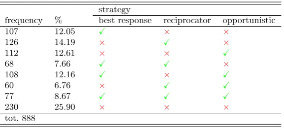
[image:21.595.159.448.107.239.2]

tot. 888

Table 2: The table shows the frequency of choices in our experimental sample explained by each of the three strategies alone and all possible overlaps. The tick indicates when a strategy is represented; the cross when it is not

strategy at random in each round, given the network arisen in the previous round, we notice

that similarly to what observed in the case of best responders, reciprocators (opportunists)

seem to be selecting their strategies deliberately. More in detail, the average proportion of

choices which account for reciprocator choices is 0.2420 (s.e. 0.0071), compared to 0.3727 in

our experimental sample; the average proportion of choices which account for opportunistic

choices is, similarly, 0.2426 (s.e. 0.0071), compared to 0.4020 in our experimental sample.

Many choices can be explained by more than one strategy at a time both in the real

and the simulated samples: there are instances when the reciprocator strategy coincides

with a best response, an opportunistic strategy or both; there are other instances when

reciprocator and opportunistic strategies coincide, or do not coincide, with best response

behaviour, and so forth. Table 2 shows the overlap between the strategies arising from our

experimental sample.15 The table shows that almost 39% of all choices can be ascribed to

only one behavioural type, the remainder being explained by none of the three types, two

types at a time or three. It also reveals that 74% of all choices in our experimental sample

can be explained in the light of one of our three behavioural types. This is quite a high

proportion considering that in many cases playing a certain strategy in such a game might

be rather difficult.

By comparing average profits obtained through each of the three strategies, we find that

15_{In table 2, the first row shows, e.g., that 107 (12.05%) choices in the experimental sample can be accounted}

(22)

100

150

200

250

average profit

1 2 3 4 5 6 7 8 9

session

[image:22.595.170.435.108.299.2]

best response reciprocator opportunistic

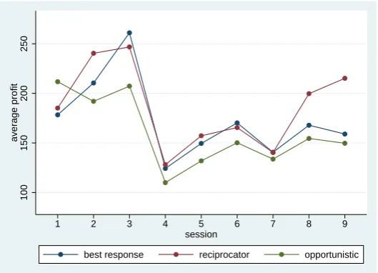
Figure 4: The figure shows average profits by strategy and by session.

the average profits obtained by best response choices are not significantly different from those

obtained by reciprocators, but both best responders and reciprocators earned, on average,

a profit larger than that earned by opportunists: best response choices yielded our

exper-imental subjects an average of 175.056 (s.e. 7.901) experexper-imental units, while reciprocators

earned 182.931 (s.e. 7.433) and opportunists 158.655 (s.e. 7.344) experimental units. Figure

4 shows that this pattern holds not just on average, but also for most sessions. The fact that

opportunists earned on average less than myopic best responders and reciprocators should

not be too surprising. Given our parametric assumptions, connections are always profitable:

indirect connections are more profitable than direct links, however both increase profits. The

opportunist, by only targeting those connections that provide the highest payoff, may often

miss out on linking opportunities by not reciprocating link proposals to those who would

bring in a more modest, but still positive, payoff.

6 The Mixture Assumption

As seen in the last section, patterns of behaviour often overlap so that the choice of a particular

strategy is compatible with more than one behavioural rule. For this reason, discriminating

(23)

the strategies selected by them. In this section, we want to verify whether subjects

system-atically adopt one of the three patterns of behaviours under investigation so that the former

can be framed alternatively within our definitions of the reciprocator type (RC), the best response type (BR) and the opportunistic type (OP). In order to assign subjects to these types, we estimate a finite mixture model (see McLachlan and Peel (2000)) that will allow us

to verify if these strategies are well identified and separated in our sample.

We proceed by assuming that a proportion πBR of the population from which the

ex-perimental sample is drawn behaves according to the best response type; a proportion πRC

behaves according to the reciprocator type; and finally a proportionπOP = 1−(πBR+πRC)

behaves according to the opportunistic type. Our mixture assumption is that each subject

belongs to one of these types and that she cannot switch type across rounds. The parameters

(πBR, πRC, πOP) are known as the mixing proportions and are estimated along with the other

parameters of the model.

The likelihood contribution of subject ithen is:

(1) Lig =πBR×lBRig +πRC×lRCig +πOP ×lOPig ,

wherelBR_ig ,l_igRC and lOP_ig are the likelihood contributions of individualiunder the hypothesis of her belonging to the best response type, the reciprocator type and the opportunistic type,

respectively. These are derived as follows.

We model the individual propensities to behave according to type h ∈(BR, RC, OP) in a very simple way, that is, by assuming that there is an average propensity,γ_gh, to choose one of the strategies that comply with that type’s rule which is common to all the subjects of

that type. γ_gh has a subscriptg because we allow it to vary across groups in order to capture possible coordination effects (group-specific fixed effects). In other words, we test whether

players are more likely to adopt a strategy if there are other players in her group of the same

(24)

his:

yh_ig,t∗ = γ_gh+εh_ig,t i= 1, . . . ,6 g= 1, . . . ,9 t= 1, . . . , Tg

(2)

εh_ig,t ∼ N[0,1]

Here, εig,t is an error term, distributed as a standard normal and independent of anything

else in the model. yh_ig,t∗ is a latent variable representing playeri’s attitude to act according to strategic type h. The available data is an unbalanced panel since the number of rounds in each session (Tc) depends on a random stopping rule that decides, after round 15, whether or

not to continue with another round of the game.

The observational rule is the following:

y_ig,th = 1 ifsig,t complies with type h’s behavioural rules

y_ig,th = −1 otherwise

The likelihood contribution of subjecti, conditional on being of type h, is

(3) lh_ig =Lh_ig

γ_gh |sig,1, . . . , sig,Tg

=

Tg

Y

t=1

Φ

h

y_ig,th ×γ_gh

i

,

where Φ [·] is the standard normal cumulative distribution function.

Results are displayed in Table 3. In specification 1, where allγ_gh, withh∈(BR, RC, OP), are estimated as common constants, we find that the predominant type is the best response

type, followed by the reciprocator and the opportunistic type. Adding group fixed effects to

the three types significantly increases the log-likelihood according to the likelihood-ratio test

(χ2₂₄= 80.010,p-value<0.0001). This makes again the best response type the most popular with a mixing proportionπBR= 0.452, followed by the reciprocator type with aπRC= 0.296

and the opportunistic type with a πOP = 0.252. Compatible with these results, we observe

that adopting a certain strategy seems group-driven (e.g., players are more likely to best

respond if they are in a group where there are other players who do best response).

(25)

probabil-(1) (2)

γBR _CC _{GF E}

γRC _CC _{GF E}

γOP CC GF E

πBR 0.417 0.452

(0.090) (0.087)

πRC 0.367 0.296

(0.090) (0.073)

πOP 0.216 0.252

(0.072) (0.073)

[image:25.595.97.499.408.471.2]

Log-likelihood -512.645 -472.640 observations 888 888 number of subjects 54 54 number of groups 9 9

Table 3: Estimation results of the mixture model. CCindicates that a common constant is estimated;GF E indicates that group fixed effects are estimated. The results are omitted.

All mixing proportions are statistically significant at 1% level.

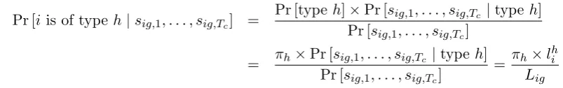
ities of each experimental subject being of each type. Using Bayes’ rule we have the following

posterior probabilities:

Pr [iis of type h|sig,1, . . . , sig,Tc] =

Pr [type h]×Pr [sig,1, . . . , sig,Tc |type h]

Pr [sig,1, . . . , sig,Tc]

= πh×Pr [sig,1, . . . , sig,Tc |type h]

Pr [sig,1, . . . , sig,Tc]

= πh×l

h i

Lig

(4)

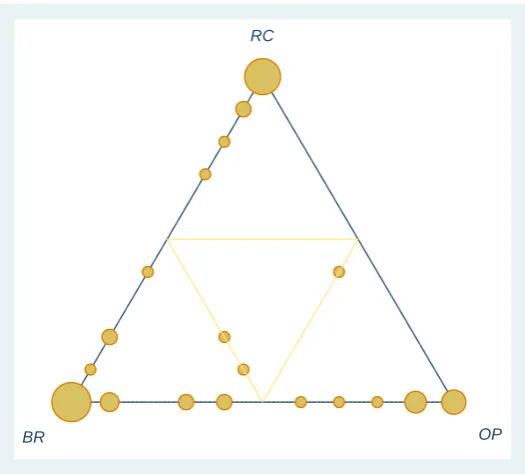
forh∈ {BR, RC, OP}.Posterior probabilities are reported on the simplex displayed in Figure 5. The 54 subjects are represented by circles in the graph: small circles represent a single

subject; larger circles cluster subjects concentrated in that area of the simplex (the larger

the circle the more numerous the cluster). The closer a subject is to a vertex of the simplex

the greater the posterior probability for that subject of being of the type represented on that

vertex.16 Subjects in the bottom left corner are of the best response type; subjects in the

top corner are of the reciprocator type and, finally, those in the bottom right corner are of

the opportunistic type. The majority of subjects are located very close to the vertices of

the simplex, a minority to the edges and only three are in the middle. The yellow simplex

in the centre represents a virtual area of “uncertainty over types” and is empty in the case

under examination. This finding confirms that the mixture model clearly separates the three

16

(26)

BR

RC

[image:26.595.170.433.107.344.2]

OP

Figure 5: Posterior probability of types from estimation results in Table 3, specification 2.

types of individuals, with most of them being assigned to a particular type with quite a high

posterior probability.17

7 Conclusions

In this paper we use experimentally generated data to analyse individual linking strategies in

a network formation game.

By a system of equations modelling players’ link proposals in each round of the game,

we are able to distinguish between strategies that we name of the reciprocator type, of the

myopic best response type and of the opportunistic type.

We find that approximately 40% of the network formation strategies adopted by the

exper-imental subjects can be accounted for as myopic best response strategies, 37% as reciprocator

strategies and 40% as opportunistic strategies. Adding myopic best response, reciprocator and

opportunistic behaviour, we are able to explain approximately 74% of the observed choices.

We show that each of these types of behaviour is ‘deliberate’ in that we have obtained shares

17

(27)

of each behaviour that are significantly different from what we would have obtained if agents

had selected links at random.

Given that there is overlap between strategies, we have tested econometrically if a mixture

assumption can be validated for our sample. We find that it is safe to assume that each

individual belongs to one type, with mixing proportions approximately equal to 45%, 30%

and 25% for best response, reciprocator and opportunistic types, respectively.

We observe that the average profits obtained by subjects following each of the strategies

are not too dissimilar, with opportunists earning marginally less. We argue that this is

because, by targeting only the links which have the highest connectivity, opportunists may

miss out on profitable connections.

Finally, we discover that the individual attitude to adopt a certain strategy is heavily

group-driven, with agents being more likely to best respond, for example, when others in the

same group also do so.

The latter finding has very interesting policy implications. By having more subjects who

have an individual propensity toward a certain behaviour, we increase the attitude to adopt

that kind of behaviour of other members of the same group. Hence by controlling the group

composition in behavioural types one could favour some network outcomes as opposed to

others.

In this paper, we present the reciprocator and the opportunist as behavioural strategies

other than myopic best response behaviour. If agents are myopic and have static expectations,

anything other than myopic best response is ‘irrational’. In a more complex model, where

agents are farsighted and averse to strategic uncertainty, rational behaviour may share features

with the strategies that we have outlined here. A rational farsighted agent may attempt

to establish her reputation as a reliable connection by always reciprocating link proposals.

Equally, an agent who is averse to strategic uncertainty may choose to keep redundant links.

We do not attempt such modelling here, but acknowledge the possibility that in a more

general model of network formation the behavioural patters we outline here may indeed stem

(28)

Appendix A. The econometric model of link proposals

In each round of the game, each subject submits a vector of choices concerning the opportunity

to propose or not propose a link to any of her opponents. From a player’s perspective, the

decision to propose a link to one of her opponents is not separate from the decision to propose

or not propose a link to another opponent. For this reason, all decisions made by a player

in a round are not independent but they are the result of a joint evaluation and need to be

analysed as such.18

Let us consider a set of 6 players, indexed byi= 1, . . . ,6. Each playeri in roundt submits a 5-dimensional vector of intended links:

sig,t= (si1g,t, . . . , sijg,t, . . . , si5g,t).

Here, j = 1, . . . ,5 represents i’s prospective players; groups of opponents are indexed by g,

withg= 1, . . . ,9;t= 2, . . . , Tgindicates the round number. The final round number,Tg, may

differ by group because of a random stopping rule that decides, after round t= 15, whether or not to continue with another round of the game. sijg,t equals 1 if subject i expresses his

willingness to be linked toj; it equals−1 otherwise.

The vector of intended links sigt is the result of a complex decision process. In making

her decisions, i needs to jointly evaluate the opportunity to propose a link to each of her 5 prospective players. In other words, ineeds to consider the following system of equations:

s∗_ijg,t = αi+λg+β

0

wWijg,t−1+β

0

xXjg,t−1+β

0

yYig,t−1+β

0

zZg,t−1+

uijg,t

(1 +δ(t−2)), for j = 1, . . . ,5 and j6=i.

(5)

Here, Wijg,t−1 is a vector of explanatory variables describing the characteristics of the

re-lationship between i and j in the previous round, including the lagged dependent variable,

sijg,t−1;Xjg,t−1 is a vector of characteristics ofjas shown by the network that emerged in the

previous round; Yig,t−1 is a vector of explanatory variables related to i’s position in the net-18

(29)

work in the previous round; the explanatory variables inZg,t−1 describe the main features of

the network resulting from players’ link proposals in the previous round. There are also two

regression intercepts, αi and λg. Intercept αi varies across individuals (individual-specific

time-invariant random effect) and is assumed to be common to all equations in (5). We

also assume that it does not depend on any observable. It represents the individual-specific

propensity to demand links and is assumed to be distributed normal across the population:

αi ∼N 0, σα2

. In a network formation game, individual decisions within a group may well

be correlated because of unobservable common shocks to all individuals in the same group

– for example, because all individuals observe the same sequence of graphs occurring during

a session. Our method of controlling for dependence on unobservables within a session is

to model the intercepts λg as random unobservables (group-specific fixed effects). The term

(1 +δ(t−2)) is introduced in order to capture the effect of experience on players’ decisions. A positive (negative)δ implies that subjects’ choices eventually become less (more) noisy.19

s∗_ijg,t– the latent dependent variable representing subject’sipropensity to demand a link toj

– andsijg,t, the observed binary outcome variable, are related by the following observational

rule:

sijg,t=

  

 

1 ifs∗_ijg,t≥0

−1 else

.

Since players in each round jointly evaluate the opportunity to propose a link to any

of their opponents, we expect that the choice of proposing a link to one of the prospective

partners reduces the probability of proposing a link to the others. In other words, we expect

to observe a negative correlation across the equations in (5).20 i’s decision in each round can be framed within the class of M-equation multivariate dynamic probit models. Anyhow,

we need to place some restrictions on the variance-covariance matrix of the errors and the

19

A positive δwould eventually reduce the error variance (that is constrained to be equal to 1 in round 2 for identification purposes), consequently making the role of the stochastic disturbance less and less relevant in players’ decisions and, in this sense, highlighting the role of experience accumulated throughout the game.

20

(30)

coefficients on the system’s variables. In particular, the joint distribution of the error terms

is assumed to take the form:

V            

ui1g,t

.. .

uijg,t

.. .

ui5g,t

            =            

1 · · · ρ · · · ρ

..

. . .. ... ... ...

ρ · · · 1 · · · ρ

..

. . .. ... ... ...

ρ · · · ρ · · · 1

            . (6)

Here, error variances on the leading diagonal of V have values of 1 and the off-diagonal

elements are all equal to ρ. This hypothesis of equi-correlation of the error terms of the system of behavioural equations (5) follows from the fact that there is no reason to assume

that a certain pair of equations in (5) are more or less correlated than another pair. Further,

we assume that the coefficients on the variables in system (5) do not vary across equations.

Estimation of the dynamic system (5) requires an assumption about the initial

observa-tions sijg,1. Since players do not know anything about their opponents and the group of

players as a whole before the graph of the network resulting from round 1 link proposals is

shown to them, we can safely assume that the initial conditionsijg,1 is completely random.

Let us define playeri’s likelihood contribution as:

Lig =

Z ∞

−∞

Tg

Y

t=1

Φ5(µig,t; Ω)f α; 0, σ2α

dα,

(7)

where µig,t= (si1g,t×µi1g,t, . . . , sijg,t×µijg,t, . . . , si5g,t×µi5g,t) and µijg,t= (1 +δ(t−2))×

αi+λg+β

0

wWijg,t−1+β

0

xXjg,t−1+β

0

yYig,t−1+β

0

zZg,t−1

, with j = 1, . . . ,5; Ω is a sym-metric 5 ×5 matrix whose elements on the leading diagonal are equal to 1 (σjj = 1 for

j = 1, . . . ,5) and are equal toσjk =sijg,t×sikg,t×ρ(forj, k= 1, . . . ,5 andj6=k) somewhere

else; f α; 0, σ2

α

is the normal density function with mean 0 and varianceσ2

α evaluated atα.

The multivariate normal cumulative distribution function Φ5(.) is evaluated by the

Geweke-Hajivassiliou-Keane (GHK) algorithm.21 The likelihood function is maximised using 20-point

21

(31)

Gauss-Hermite quadrature.22

Appendix B. Experimental instructions

Welcome

This is an experiment on the formation of links among different subjects. If you make

good choices you will be able to earn a sum of money that will paid to you in cash immediately

after the end of this session.

You are one of 6 participants to this experiment; at the very beginning the computer will

randomly assign to you an initial budget (equal across participants). The computer will also

randomly assign to you an icon (Dropper,Radio,Cube,Floppy disk,Hand lens,Hour

glass) that will identify you throughout the experiment and will assign you an initial budget

(equal across participants). The icon identifying you is circled in red on your screen.

The experiment consists of a random number of rounds: there will be at least 15 rounds,

after which a lottery administered by the computer will determine whether there will be a

further round or the experiment is over.

Each participant to this experiment represents a node. At the beginning of the experiment

all nodes are isolated. In each round, the computer will ask you whether you want to propose

any link and to whom. You may propose 0, 1 or more links. The computer will collect the

proposals from all participants and activate only the links desired by both of the two subjects

involved (reciprocated proposals).

Your screen will show the graph of active links. The box at the bottom right corner of

your screen will show you who has proposed a link to you in the previous round and to whom

you have not reciprocated.

Each link that you manage to activate has a cost (equal across participants) that is

indicated on the screen. In each round, the computer may reject your link proposals if they

entail an expenditure that is higher than your budget for that round.

Your revenues in each round are automatically computed and are given by the product by

the revenue per node (equal across subjects and indicated on your screen) and the number

(32)

of nodes that you manage to reach both through your direct links and the links activated by

other participants.

Computing costs and revenues

Example: subject Radio is directly linked to Floppy disk and Dropper and indirectly,

that is throughDropper, toHand lens.

In each round, the computer calculate out your profit and display it on your screen. The

overall profit from the experiment is given by the sum of your revenues in all rounds. At the

end of the experiment, you will be paid in cash an amount in euros equivalent to 10% of your

total profit.

References

Bala,V., Goyal, S., 2000. A Non-Cooperative Model of Network Formation. Econometrica,

68(5):1181–1229.

Bernasconi, M., Galizzi, M., 2012. Networks, Learning Cognition, and Economics.

Encyclo-pedia of the Sciences of Learning, 2440–2443.

Bloch, F. and Jackson, M., 2006. Definitions of equilibrium in network formation games.

International Journal of Game Theory, 34:305–318.

Berninghaus, S.K., Ott, M., Erhart, K.M., Vogt, B., 2007. Evolution of networks - an

experimental analysis. Journal of Evolutionary Economics, 17:317–347.

Callander, S. and Plott, C., 2005. Principles of Network Development and Evolution: An

experimental Study. Journal of Public Economics, 89(8):1469–1495.

Calv´o-Armengol, A., 2004. Job contact networks. Journal of Economic Theory, 115:191-206.

Calv´o-Armengol, A. and Ilkilic, R., 2009. Pairwise-stability and Nash Equilibrium in

Net-work Formation. International Journal of Game Theory, 38:51–79.

Cappellari, L., Jenkins, S.P., 2006. Calculation of multivariate normal probabilities by

sim-ulation, with applications to maximum simulated likelihood estimation. Stata Journal,

6(2):156–189.

Carrillo, J.D. and Gaduh, A., 2011. The Strategic Formation of Networks: Experimental

Evidence, CEPR Discussion Paper n. DP8757.

Conte, A., Moffatt, P.G., 2014. The econometric modelling of social preferences. Theory

and Decision, 76(1):119–145.

Conte, A., Levati, M.V., 2014. Use of data on planned contributions and stated beliefs in

(36)

Di Cagno, D., Sciubba, E., 2008. The Determinants of Individual Behaviour in Network

Formation: Some Experimental Evidence. M.Abdellaoui and J.D. Hey (eds), Springer,

Theory and Decision Library, Cambridge.

Falk, A., Kosfeld, M., 2012. Its all about connections: Evidence on network formation.

Review of Network Economics, 11(3):art. 2.

Goeree, J.K., Riedl, A. and Ule, A. 2009. In Search of Stars: Network Formation among

Heterogeneous Agents. Games and Economic Behavior, 67:445–466.

Goyal, S., Joshi, S., 2006. Unequal connections. International Journal of Game Theory,

34:319–349.

Jackson, M.O., Wolinsky, A., 1996. A Strategic Model of Social and Economic Networks.

Journal of Economic Theory, 71(1):44–74.

Kirchsteiger, G., Mantovani, M., Mauleon, A. and Vannetelbosch, V., 2011. Myopic or

Far-sighted? An Experiment on Network Formation, CEPR Discussion Paper n. DP8263.

McLachlan, G., Peel, D., 2001. Finite Mixture Models. Wiley and Sons, New York.

Myerson, R.B., 1991. Game theory: analysis of conflict. Harvard University Press,