Using Harmonic Mean to Solve Multi Objective Linear Programming Problems

http://dx.doi.org/10.4236/ajor.2016.61004

How to cite this paper:Sulaiman, N.A. and Mustafa, R.B. (2016) Using Harmonic Mean to Solve Multi-Objective Linear Pro-gramming Problems. American Journal of Operations Research, 6, 25-30. http://dx.doi.org/10.4236/ajor.2016.61004

Using Harmonic Mean to Solve

Multi-Objective Linear

Programming Problems

Nejmaddin A. Sulaiman, Rebaz B. Mustafa

*

Department of Mathematics, College of Education, University of Salahaddin, Erbil, Iraq

Received 11 November 2015; accepted 15 January 2016; published 20 January 2016

Copyright © 2016 by authors and Scientific Research Publishing Inc.

This work is licensed under the Creative Commons Attribution International License (CC BY). http://creativecommons.org/licenses/by/4.0/

Abstract

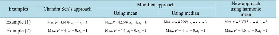
In this paper, we have suggested a new technique to transform multi-objective linear program-ming problem (MOLPP) to the single objective linear programprogram-ming problem by using Harmonic mean for values of function and an algorithm is suggested for its solution, the computer applica-tion of algorithm has been demonstrated by solving some numerical examples. We have used some other techniques, such as (sen, arithmetic mean, median) to solve the same problems, the results in Table 3 indicate that the new technique in general is promising.

Keywords

MOLPP, Harmonic Mean

1. Introduction

Linear programming is a relatively new mathematical discipline, dating from the invention of the simplex me-thod by G. B. Dantzig in 1947. He proposed the simplex algorithm as an efficient meme-thod to solve a linear pro-gramming problem.

A multi-objective linear programming problem is introduced by Chandra Sen [1] and suggests an approach to construct the multi-objective function under the limitation that the optimum value of individual problem was greater than zero. [2] studied the multi-objective function by solving the multi-objective programming problem, using mean and mean value. [3] solved the multi objective fractional programming problem by Chandra Sen’s technique. In order to extend this work, we have defined a multi-objective linear programming problem and

vestigated the algorithm to solve linear programming problem for multi-objective functions. By new technique, we use harmonic mean (HM) of the values of objective functions. The computer application of our algorithm has also been discussed by solving some numerical examples. Finally we have showed results and comparison among the new technique and Chandra Sen’s approach [1] and Sulaiman’s approach [2].

2. Mathematical Definition of Multi-Objective Programming Problems (MOPP)

A deterministic (MOPP) model is usually formulated to maximize and/or minimize several objectives simulta-neously subject to a constraint set with “≥” and/or “≤” relationships the equality constraints may be expressed as a combination of both of inequality constraints.

Mathematically, the MOPP problems can be defined as:

Max. 1, ,

Min. 1, ,

i i i

i i i

f c X i r

f c X i r s

α α

= + = _



= + = + _



 (1.1)

subject to:

AX B

≥    ₌    ≤  

(1.2)

0

X ≥ (1.3)

where x is an n-dimensional vector of decision variables c is n-dimensional vector of constants, B is m-dimen- sional vector of constants, r is the number of objective function to be maximized, s the number of objective function to maximized plus minimized,

(

s−r

)

is the number of objective that is to be minimized, A is a

(

m n×

)

matrix of coefficients all vectors are assumed to be column vectors unless transposed,

(

1, ,

)

i i s

α

=  are scalar constants, c Xi +

α

i

(

i=1,,s

)

are linear factors for all feasible solutions [3].

If α =i 0; for all i=1,,s, then the mathematical form become:

Max. 1, ,

Min. 1, ,

i i i

i i i

f c X i r

f c X i r s

α α

= + =

= + = +

  



 (2.1)

subject to:

AX =B (2.2) 0

X ≥ _(2.3)

The problem said to be multi-objective linear programming problem (MOLPP) if all the objective functions and constraint functions are linear, and all the variables are continuous variables.

3. The New Technique for Solving MOLPP by Using Harmonic Mean

Before solving MOLPP, and preface an algorithm to it, we will need to define Harmonic Mean.

Harmonic Mean [4]

Harmonic mean of a set of observations is defined as the reciprocal of the arithmetic average of the reciprocal of

the given values. If x x₁, ₂,,xn are n observations,

1

1

n

i i

n HM

x =

=

     

∑

4. Multi-Objective Functions Formulation

1 1

2 2

1 1

Max. Max.

Max. Min.

Min.

r r

r r

s s

f

f

f

f

f

+ +

= 

     Ψ = Ψ

= Ψ = _

   Ψ

= Ψ





(3.1)

where Ψi,

(

i=1, 2,,s

)

are the values of objective functions.

We require the common set of decision variable to be the best compromising optimal solution [5]. Here we can determine the common set of decision variables from the following combined objective function.

Formulate the multi-objective linear programming problem given in (1.1) can be translated by our technique to:

(

)

1

(

)

2

1 1

Max.F =

∑

rk= Max. fk Hm −

∑

k rs= + Min. fk Hm (3.2)

where

(

)

(

)

(

)

1 11 , 2 11

r s

i i

i i r

Hm =r

∑

₌ Ψ Hm = s−r

∑

_{= +} Ψ (3.3)

And Ψ ≠i 0;

(

i=1, 2,,s

)

subject to the same constraints (1.2), (1.3) and the optimum value of the

func-tions Ψ_k

(

k=1, 2,,s

)

may be positive or negative, Hm₁ the value of harmonic mean of maximized

(

1, 2, ,

)

k k r

Ψ = _ and Hm₂ the value of harmonic mean of minimized Ψk

(

k= +r 1,,s

)

. s− ≥r 2, if

1

s− =r then the combined formula (3.2) becomes.

(

)

1

(

1

)

1

1

Max.F =

∑

kr= Max. fk Hm − Min. fr+ Ψr+

If s− =r 0 then the function

(

)

₁

1

Max. r Max. _k

k

F=

∑

₌ f Hm . We can solve this (MOLPP) by Chandra

Sen’s approach [1]-[3] by using mean and median and algorithms in above researches for solving MOLPP as explained in [1]-[3].

4.1. Algorithm

This algorithm is to obtain the optimal solution for the MOLPP defined previously can be summarized as fol-lows.

Step 1: Assign arbitrary values to each of the individual objective functions that to be maximized and mini-mized.

Step 2: Solve the first objective function {Max. f₁ subject to constraints (1.2) and (1.3)} by simplex method. Step 3: Check the feasibility of the solution in step 2, if it is feasible then go to step 4, otherwise, use dual simplex method to remove infeasibility.

Step 4: Assign a name to the optimum value of the first objective function f1 say Ψ₁ Step 5: Repeat step 2, for i=1,,r for the kth objective function, for all i= +i 1,,s

Step 6: Determine Harmonic Mean Hm1 for Ψi,i=1,,r and Hm2 for i= +r 1,,s

Step 7: Optimize the combined objective function

(

)

₁

(

)

₂

1 1

Max. r Max. _k s Min. _k

k k r

F=

∑

₌ f Hm −

∑

_{= +} f Hm

under the same constraints (1.2) and (1.3) by repeating Steps 2-4.

4.2. Used Notation

The following notations were used in our algorithm:

, 1, 2, ,

i i

HA = ΨA ∀ =i  r

, 1, ,

i i

where ΨA_i = The value of objective function which is to be maximized, and

i

L

Ψ = The value of objective function which is to be minimized.

1

Hm = The value of Harmonic mean of maximized

(

₁

(

)

)

11

r i i

Hm =r

∑

₌ Ψ .

2

Hm = The value of Harmonic mean of minimized

(

₂

(

)

(

)

)

11

s i i r

Hm = s−r

∑

_{= +} Ψ .

1 1

Max. ; Min.

r s

i i

i i r

SL f SS f

= = +

=

∑

=

∑

Max.F=SL Hm1−SS Hm2

4.3. Numerical Examples

Ex. (1)

1 1 2 2 1 3 1 2 4 2

Max. 2

Max. 3

Min. 2 3

Min.

f x x

f x

f x x

f x = +   = _  = − − _  = − _ (4.1) s.to: 1 2 1 2 1 2 1 2

6 8 48

3 4 3 , 0 x x x x x x x x + ≤   + ≥ _  ≤   ≤ _  ≥ _ (4.2) Solution:

After finding the value of each of individual objective function by simplex method the results as below in (Table 1):

{

Ψ =₁ 10,Ψ = Ψ = −₂ 4, ₃ 17,Ψ = −₄ 3

}

by using Harmonic Mean technique (3.3) we get Hm₁=80 14 and

2 51 10

Hm =

After that using equation (3.2) for transform we get:

( )

1 2

Subject to given c

Max. 0.7421 1.134

onstraints 5.2 : 3

F= x + x _



 (4.3) Solving (4.3) by simplex method we get:

Max.F=6.3715 x1=4, x2=3

Solve (4.1) by:

1. Using Chandra Sen’s approach, [1]: after convert the MOLPP to the single objective problem we get

1 2

Max.F =0.4676x +0.7098x subject to the same constraints (4.2) by simplex method it is optimal solution

1 2

Max.F =3.9999 x =4,x =3.

Table 1.Results of example (1).

2. Using modified approach, [2]:

A-using Mean: after convert the MOLPP to the single objective problem we get Max.F=0.4857x₁+0.7857x₂

subject to the same constraints (4.2) by simplex method it is optimal solution Max.F =4.2999 x₁=4,x₂ =3

B-using Median: after convert the MOLPP to the single objective problem we get

1 2

Max.F =0.4857x +0.7857x subject to the same constraints (4.2) by simplex method it is optimal solution

1 2

Max.F =4.2999 x =4,x =3.

Ex. (2)

1 1

2 1 2 3 2 4 2 5 1 2

Max.

Max. 2 2

Max. 3

Min. 3

Min. 3

f x

f x x

f x

f x

f x x

= = + + = + =

   

− = − −

   

(5.1)

Subject to:

1 2 1 1 2 1 2

2 3 6

4

2 2

, 0

x x

x

x x

x x

+ 

   ≤ ≤

+ ≤

≥   

(5.2)

Solution:

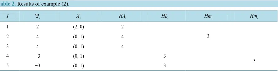
After finding the value of each of individual objective function by simplex method the results as below in (Table 2):

{

Ψ = Ψ = Ψ = Ψ = −₁ 2, ₂ 4, ₃ 4, ₄ 3 andΨ = −₅ 3

}

by using Harmonic Mean technique (3.3) we get

1 3

Hm = and Hm₂=3.

After that using equation (3.2) for transform we get:-

( )

1 2

Subject to given constraints 6.2 :

Max.F = +5 3.5x +12x _



 (5.3) Solving (5.3) by simplex method we get:

1 2

Max.F =4.6 x =0, x =1

Solve (5.1) by:

1. using Chandra Sen approach, [1]: after convert the MOLPP to the single objective problem we get

1 2

Max.F =1.25 1.08333+ x +2.75x subject to the same constraints (5.2) by simplex method it is optimal solu-tion Max.F =4 x₁=0,x₂=1.

2. using modified approach, [2]:

A-using Mean: after convert the MOLPP to the single objective problem we get

1 2

Max.F =1.5+0.93333x +2.9x subject to the same constraints (5.2) by simplex method it is optimal solution

1 2

Max.F =4.4 x =0,x =1.

[image:5.595.76.543.77.352.2] [image:5.595.92.539.605.720.2]

B-using Median: after convert the MOLPP to the single objective problem we get

Table 2.Results of example (2).

2

Hm

1

Hm i

HL i

HA i

X i

Ψ

I

3 2

(2, 0) 2

1

4 (0, 1)

4 2

4 (0, 1)

4 3

3 3

(0, 1) −3

4

3 (0, 1)

[image:6.595.89.543.101.159.2]

Table 3.Comparison between results obtained by different numerical approaches.

New approach using harmonic

mean Modified approach

Chandra Sen’s approach Examples

Using median Using mean

1 2

Max.F=6.3715x=4,x=3

1 2

Max.F=4.2999x=4,x=3

1 2

Max.F=4.2999x=4,x=3

1 2

Max.F=3.9999x=4,x=3

Example (1)

1 2

Max.F=4.6x=0,x =1

1 2

Max.F=4x=0,x =1

1 2

Max.F=4.4x=0,x =1

1 2

Max.F=4x=0,x =1

Example (2)

1 2

Max.F =1.25+0.83333x +2.75x subject to the same constraints (6.2) by simplex method it is optimal solu-tion Max.F=4 x₁=0,x₂=1.

5. Conclusions

Our aim was to develop an approach for solving multi-objective programming problem (MOLPP) and to suggest a new algorithm to convert the MOLPP into a single LPP by using harmonic mean of the values of objective functions and its computer application by using programming mathematical language (Matlab Programming). Moreover, we used different methods to solve the problems, and applied our technique and the other methods to the same examples in order to compare the results.

From this comparison, we observed that our technique gave identical results with that obtained by the other methods, for this see Table 3. So we conclude that this method is better than other methods considered in solv-ing MOLP problems.

References

[1] Chandra, S. (1983) A New Approach Objective Planning. The Indian Economic Journal, 30, 91-96.

[2] Sulaiman, N.A. and Sadiq Gulnar, W. (2006) Solving the Multi-Objective Programming Problem; Using Mean and Median Value. Ref. J of Comp & Math’s, 3.

[3] Abdul-Kadir, M.S. and Sulaiman, N.A. (1993) An Approach for Multi-Objective Fractional Programming Problem.

Journal of College of Education, University of Salahaddin, 3, 1-5. [4] Jothikumar, J. (2004) STATISTICS. 60 G.S.M Paper, p.100.