Munich Personal RePEc Archive
The Push-Pull Effects of the Information
Technology Boom and Bust
Hotchkiss, Julie L. and Pitts, M. Melinda and Robertson,
John C.
Federal Reserve Bank of Atlanta, Georgia State University, Andrew
Young School of Policy Studies
August 2008
The Push-Pull Effects of the Information Technology Boom and Bust:
Insight from Matched Employer-Employee Data
Julie L. Hotchkiss
Federal Reserve Bank of Atlanta and Georgia State University [email protected]
(404) 498-8198
M. Melinda Pitts
Federal Reserve Bank of Atlanta [email protected]
(404) 498-7009
John C. Robertson
Federal Reserve Bank of Atlanta [email protected]
(404) 498-8782
Research Department Federal Reserve Bank of Atlanta
1000 Peachtree Street, NE Atlanta, GA 30309-4470 Fax Number: (404) 498-8058
December 2007
The views expressed in this paper are those of the authors and do not necessarily reflect the views of the Federal Reserve Bank of Atlanta or the Federal Reserve System. The authors would like to thank Chris Cunningham, Sabrina Pabilonia, Kathryn Shaw, and Dan Wilson for their insightful suggestions, as well as participants at seminars presented at University of Colorado-Denver, University of Kansas and University of North
The Push-Pull Effects of the Information Technology Boom and Bust:
Insight from Matched Employer-Employee Data
Abstract
Biographies
Julie Hotchkissis a research economist and policy adviser at the Federal Reserve Bank of Atlanta. Her research on employment, earnings, and labor supply decisions can be found in the American Economic Review, Southern Economic Journal, and Social Service Review.
Melinda Pitts is a research economist and associate policy advisor at the Federal Reserve Bank of Atlanta. Recent research in health and labor economics is published in the American Economic Review, Southern Economic Journal, and American Journal of Managed Care.
The Push-Pull Effects of the Information Technology Boom and Bust:
Insight from Matched Employer-Employee Data
I. Introduction
The U.S. information technology (IT) sector experienced remarkable growth
during the second half of the 1990s, driven by strong business demand for IT goods and
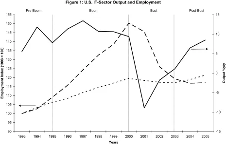
services. As shown in Figure 1, the dollar value of output of the IT-producing sector
(solid line) grew by more than 10 percent each year between 1996 and 1999. However,
IT production declined sharply in 2001 when businesses made deep cuts in IT spending.
Since 2003, IT sector production has recovered somewhat, with IT output reaching an
annual growth rate of 8.5 percent by 2005.
The boom in IT production during the 1990s led to a dramatic rise in employment
in IT-producing industries, and the subsequent contraction in IT production resulted in a
large decline in IT-sector employment in the early 2000s. Figure 1 shows that, between
1993 and 2000, the number of workers in IT-producing industries in the U.S. (dashed
line) increased by 50 percent, which is almost two and a half times as fast as the
employment gains in private sector non-IT industries (dotted line). From 2001 to 2003,
employment in IT-producing industries declined by 20 percent from the peak, compared
with a two percent decline in non-IT industries. Since 2003, employment in the IT sector
has been relatively stable, although at much lower levels than during the boom, while
non-IT employment has been expanding.
[Figure 1 here]
Although there was rapid growth in employment in the IT sector during the boom
Valetta, 2004). The concentration of IT employment growth in geographically distinct
metropolitan areas such as Washington, D.C., San Francisco, Austin, Boston, Seattle,
Phoenix, and Atlanta presents these areas as unique laboratories in which to investigate
the impact of extraordinary swings in labor demand on movements of individuals into
and out of local labor markets. Moreover, Cortright and Mayer (2001) show that
metropolitan areas varied considerably in their areas of specialization within the IT
sector. For instance, Atlanta was identified as having a relatively high concentration in
software development but a low concentration in IT manufacturing. In contrast, Phoenix
was identified as a center for hardware rather than software development. This suggests
there was considerable heterogeneity in the types of workers attracted to different IT
centers. In turn, the variation in the skill sets of these workers likely impacts their ability
to transition into other sectors during industry-specific as well as general economic
downturns. For example, Hart (2007) observes that IT-manufacturing industries are often
characterized by semi-skilled workers while hardware and software development are
characterized by high skilled workers. Thus, following an employment shock,
IT-manufacturing workers are expected to act more like workers in other IT-manufacturing
industries than workers in IT services such as software and system design.
The purpose of this paper is to investigate whether the flow of individuals into a
local workforce in response to a substantial increase in employment opportunities in the
IT sector was matched by a comparable outflow when those specific opportunities
evaporated. Research has established a fairly stable positive relationship between the
skill level of an area's workforce (as measured by educational attainment) and the growth
often been viewed as a goal of local economic development efforts, and local public
funds are often used to attract new businesses in particular high-skilled industries.
However, if skilled workers exit the local workforce when businesses fail, then the
economic gain is only as long-lived as the businesses themselves. If, on the other hand,
skilled workers have staying power beyond the original attraction to the local workforce,
the economic benefits of a skilled workforce accrue beyond the life of the initial
opportunities.
The pull on individuals to geographic areas experiencing positive economic
growth and the push of individuals out during economic declines has been referred to as
"push-pull" migration, and has been analyzed in a variety of different contexts.1 For the
purposes of this paper, migration will be considered in the context of entry and exit from
the workforce in the state of Georgia, with the IT sector’s boom providing the pull of
individuals with IT skills into Georgia's workforce, and the subsequent decline as the
potential push out. Hotchkiss, Pitts, and Robertson (2006) demonstrate that the patterns
in IT and non-IT employment in Georgia closely resemble those for the US displayed in
Figure 1. Using matched employer-employee payroll data for Georgia over the period
1993-2005, the analysis in this paper finds that workers in the Software and Computer
Services industry were disproportionately more likely to be new workforce entrants
during the IT boom, but were not any more or less likely to exit the workforce during the
IT bust. The implication is that the pull of employment opportunities in the IT-producing
sector was much stronger than the push of declining opportunities in that sector during
producing industries (see DeBacker, Hotchkiss, Pitts, and Robertson, 2005), may bode
well for long-term economic benefits of attracting high-skilled workers.
II. Theoretical Framework
The goal of the analysis in this paper is to determine whether the dramatic swings
in demand for workers in the IT-producing sector caused individuals to be more likely to
enter the state's workforce during the boom and more likely to exit after the boom ended
relative to workers in other industries. There are two ways in which workers are
observed entering or exiting the Georgia workforce. The first is through physical
migration and the second is through changes in residents' decisions to participate in the
labor market. While the data do not allow for the distinction between these two sources,
the actions are guided by the same utility maximizing framework.
A. Migration
Basic migration theory models the decision to migrate as an investment decision
(e.g., Schultz, 1961, Becker, 1964, and Mincer and Jovanovic, 1981). The net present
value of migrating (NPVM) is determined by evaluating the difference in the returns to
moving and the cost of that move:
(
)
(1 )
T
B B A A
M t
t
w w
NPV C
r
π π
⎡ − ⎤
= ⎢ ⎥−
+
⎣ ⎦
∑
. (1)The returns to moving from location A to location B are depicted as the present value of
the expected wage in location B, which is equal to the probability of finding employment
discount factor; T is the amount of time spent in location B; and C represents the cost of
the move. There is a vast literature that establishes how the total cost of migration is
dependant upon the characteristics of the worker and the amenities of the geographic
locations being compared (for example, see Greenwood, 1985, Hunt, 1993, and Gabriel
and Schmitz, 1995). For example, the greater the distance between location A and
location B the higher the cost of moving, and people with more education apparently
experience lower (psychic and informational) costs (see Schwartz, 1973).
For the purposes of this analysis, it is expected that the unprecedented growth in
demand for IT workers in Georgia during the IT boom affected migration decisions
throughπB, and perhaps throughwB. Certainly, the growth in demand for workers,
ceteris paribus, increases the probability of finding employment and may also be large
enough, relative to the supply of workers, to bid up wages. So, for any given
employment opportunities in the original geographic location (outside of Georgia) and
any given costs associated with moving to Georgia, the net present value of migrating to
Georgia would be higher during the IT boom than during other periods, increasing the
likelihood of migration.
This type of migration is often referred to as "pull-migration," as the economic
rewards in location B "pull" workers to that location. As the boom turns into a bust, and
industry demand for workers in location B falls, there may be an analogous "push" out of
the local workforce. The existing push-pull literature typically finds pull factors are
B. Labor Force Participation
In addition to physical migration into Georgia, the workforce can grow as a result
of residents of Georgia re-assessing their labor force participation decisions. The
standard labor/leisure choice model assumes that a person maximizes utility over two
goods, income and leisure:
max ( , )
L
U =U Y L , (2)
with U(.) increasing in both expected income (Y) and leisure (L). There is a tradeoff
between income and leisure summarized by the budget constraint:
*
0 ( )
Y =Y + E−L w , (3)
where Y0 is a person's non-labor income, E is the endowment of time that a person has
available to work, and w* is the person's expected wage and reflects the cost of one hour
of leisure. The expected wage, as in equation (1), can be thought of as the product of the
value of the person's human capital (the actual market wage for that person, w) and the
probability that the person can find a job (π):
*
w =wπ. (4)
The well-known optimizing solution to the labor/leisure choice model is that a
person will choose to enter the workforce if the expected wage exceeds his/her
reservation, which is defined as the marginal rate of substitution (MRS) between income
and leisure at zero hours of work (L=E):
*
if L E
L E w MRS
=
< > . (5)
Just as with the decision to migrate, an increase in demand for workers during the
wage and labor force participation for workers with the needed skills. Here, too, there is
a large literature that ties labor force participation decisions to the strength of the labor
market (for example, see Long, 1958 and Borrow, 2004).
III. Empirical Framework
Among workers observed to be working in Georgia during the IT boom, the
decision to have entered the workforce during the boom or to exit the workforce during
the bust is operationalized by assuming that a person's assessment of the costs and
benefits of migrating into or out of a labor market can be represented by a linear function
of observable factors affecting the entrance and exit decisions:
* * '
1
0 if >0 or 1
0 otherwise 0
in
M L E i
i i i
i
NPV w MRS Enter
I X
Enter
β ε ⎧⎪> > = ⇒ =
= + =⎨ ≤ ⇒ = ⎪⎩ (6) * * ' 2
0 if >0 or 1
0 otherwise 0 out
M L E i
i i i
i
NPV w MRS Exit
Y X
Exit
α υ ⎧⎪> ≤ = ⇒ =
= + =⎨
≤ ⇒ =
⎪⎩
(7)
ji
X is a vector of observable characteristics, detailed below, that determine
individual i's net return to entering or exiting the Georgia workforce. The unobserved
random components, εi andυi, are assumed to be independent and identically distributed
according to a standard normal distribution function. Estimates for β and α are
obtained via maximum likelihood.
III. The Data and Sample Construction
The data used for the analysis are for private sector workers outside of the natural
records compiled by the Georgia Department of Labor for the purposes of administering
the state's Unemployment Insurance (UI) program. The program provides almost a
complete census of employees on non-farm payrolls, with information available on
approximately 97 percent of these employees. These data are highly confidential and
strictly limited in their distribution.
The Employer file contains records on all UI-covered firms and includes
establishment level information on the number of employees and the wage bill, as well as
the NAICS industry classification of each establishment.3 The Individual Wage file
contains information on a worker's total quarterly earnings from an employer.4 The wage
file contains no information about the worker's demographics (e.g., education, gender,
race, etc.) or about the worker's job (e.g., hours of work, weeks of work, or occupation).
However, the worker's employment experience can be tracked over time using a worker
ID number and can be linked to the Employer file via a firm ID number.5 Because the
individual wage file contains a firm, rather than an establishment, identifier, a choice of
which NAICS code to assign to each worker who was employed by a multi-establishment
firm is required. Following the Department of Labor convention, a 6-digit NAICS code
is assigned based on the largest share of the firm's total employment.
A. Time Period Definitions
The data are available from the first quarter of 1993 to the fourth quarter of 2005
(52 quarters). Because the focus is on the differences in behavior of workers across
industries during the IT-employment boom and after the boom ended, the sample is split
periods shown in Figure 1. The beginning of the boom period is defined at the point
when the growth rate in Georgia’s IT-sector employment began to deviate from the
growth in the non-IT sector, which occurred in the first quarter of 1996. The peak in
Georgia’s IT sector employment occurred in the fourth quarter of 2000, signaling the end
of the boom period.
Given that the data are available from the first quarter of 1993, the pre-boom
period is defined as all quarters from 1993 through 1995. The bust period is the period
from the first quarter of 2001 through the fourth quarter of 2002. The post-bust period is
defined to be the first quarter of 2003 to the fourth quarter of 2005.
B. Industry Definitions
The IT-producing sector is divided into three components: the manufacturing of
IT equipment or components, Software and Computer Services, and Communication
Services.6 The non-IT industries are Construction, non-IT Services (including
Transportation and Utilities, Wholesale and Retail Trade, Finance, Insurance, and Real
Estate, and Miscellaneous Non-IT Services), and non-IT Manufacturing.
The industry of employment for the worker is determined by the worker’s modal
industry, i.e. the industry in which the worker spent most of his/her employed quarters
during the boom. This concept of modal industry allows for the panel data to be
collapsed in a single cross-section which describes an individual's primary activity and
C. Full-time Worker Restriction
In defining boom-period employment, the sample is restricted to those who are
most likely to be full-time workers with at least one complete quarter of employment in
the boom period. With no information on hours of work or number of weeks worked in a
quarter, this restriction is accomplished by using only "interior" quarters of earnings to
identify employment activity. An interior quarter of earnings is a quarter with real
earnings of at least $3000 that is sandwiched between two other quarters of earnings from
the same employer.8 To assign a unique industry characteristic to each worker in the
sample the firm ID is assigned based on the employer from which the worker received
his/her greatest earnings during that quarter.
D. Defining Entry and Exit
Conditional on having at least one quarter of employment in the boom-period,
individuals are considered to have entered the Georgia workforce if they were completely
absent from the Georgia Individual Wage Files during all 12 quarters of the pre-boom
period. Likewise, individuals are considered to have exited the Georgia workforce if they
were absent from the Wage Files during all 12 quarters of the post-bust period.9 These
definitions of entry and exit are used to ensure the "cleanest" entrance and exit possible,
relative to the boom period, given the limitations of the data at hand. To require that a
worker not have been present for three years prior to the boom and for three years in the
post-bust period guards against identifying a marginally attached worker as someone
whose behavior was systematically affected by the timing of the IT boom. In addition,
adjust to the declines in employment during the bust and so that short-term job losses
associated with the IT-bust are not counted as a permanent exit from the local workforce.
A further important consideration for the interpretation of the results is that the
data do not allow for the identification of where individuals are coming from upon entry,
or where they go when they exit. An individual may be absent from the Wage File for a
number of reasons. A person absent from the Wage File may be living in Georgia, but
not working, because they are unemployed or out of the labor force (e.g., retired or in
school), or may be living outside of Georgia, either working or not. For this reason, the
results do not provide information on the specific geographic migration patterns of
individuals. However, research (for example, Greenwood, 1975) has shown that
employment opportunity is a major determinant of migration, and so it is expected that
the results are generally relevant to considerations of migration.
E. Sample Characteristics
The probability of entry/exit is modeled as a function of observed boom-period
individual characteristics: the rate of employer turnover (as an indicator of mobility),
modal industry of employment, the individual's average earnings in that industry during
the boom, and the individual's average earnings interacted with modal industry.
Pre-boom absence is also included as a regressor in probability of exit specification since one
might expect that individuals who were new to Georgia’s workforce in the boom period
may be more mobile and hence may be more willing to exit as well.
The industry of employment during the boom is the regressor of primary interest.
others have found that migration and job-changing tendencies vary across human capital
characteristics, the worker's average boom period earnings is interacted with the worker's
modal industry of employment.10 Earnings are found to vary systematically across
industries, with some of the highest paid workers being found in the IT industries. The
interaction of earnings with industry controls for human capital differences in workforce
decisions and allows for conclusions specific to industry of employment.11 The
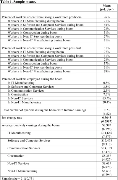
descriptive statistics for these variables are presented in Table 1.
[Table 1 here]
The 26 percent of workers that entered the Georgia workforce during the boom
mirrors the U.S. Census (2001) estimate of population growth for the state between 1990
and 2000. The 31 percent of workers who exited after the boom translates into an
average annual exit rate of 6.2 percent (this is an upper bound estimate as workers may
have exited before the year 2000). Dardia et al. (2005) found similar rates of entry and
exit in California during and after the IT boom. While the data used in this paper do not
allow us to discern the source of entry and exits, the U.S. Census Bureau (2007) estimates
that 2.7 percent of the U.S. population moved from one state to another each year
between 2000 and 2005, suggesting that transitions from employment to nonparticipation
explains about half of the annual exit rate. Frazis et al. (2005) estimate average monthly
flows of workers between employment, nonparticipation, and unemployment; the
estimation suggests that, on average across all industries, almost three percent of those
employed each month flow into nonparticipation.
Workers had an average of 0.3 different employers per quarter observed working.
Workers in construction changed jobs most frequently (every six quarters, on average)
and workers in manufacturing stayed with the same employer the longest (approximately
10 ten quarters, on average).12 The mean of average boom-period earnings was $8,993
per quarter, in 2003 dollars. Most workers were employed in non-IT Service industries
during the boom (65.5 percent), followed by non-IT Manufacturing (20.4 percent).
About seven percent of Georgia workers worked in one of the three IT-producing
industries. The highest paying industry was Software and Computer Services (an average
of $15,478 per quarter). Although Construction was the lowest paying industry (an
average of $8,356 per quarter), there was relatively very little difference in the mean of
average earnings in each of the three non-IT sectors.
The boom-period entry and exit percents show some variation across industries.
The Software and Computer Services industry and the Construction industry had the
largest share of workers that were absent from the Georgia workforce during the
1993-1995 pre-boom period. In contrast, Manufacturing workers (IT and non-IT) were the
least likely to have been absent during the pre-boom period. Construction workers were
the most likely to exit the Georgia workforce during the 2003-2005 post-bust period,
whereas manufacturing workers and communication service workers were the least likely
to have exited.
While the sample means tell us about the raw movement into and out of the
workforce by the average worker in each industry, they do not indicate whether
differences across workers in different industries are the result of the opportunities that
differ across the industries or whether they are the result of differences in the
estimation and simulations that follow yield workforce transition probabilities net of
observable worker characteristics.
IV. Predicted Probability of Entry and Exit
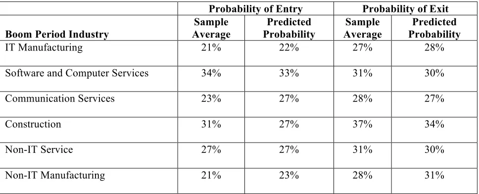
The probit estimation results for entry and exit are reported in Appendix A. Table
2 contains the average predicted probabilities of entering and exiting the Georgia
workforce constructed from the estimated parameter coefficients; the sample entry and
exit proportions by industry are also included for comparison purposes. The probability
of entry and exit for industry j was calculated for all workers as if they had been
employed in industry j during the boom, given their individual characteristics. These
individual predicted probabilities were then averaged across the entire sample to yield the
average predicted probabilities.13
[Table 2 here]
The first thing to notice in Table 2 is that there is more variation in the raw
sample averages than in the predicted probabilities. This is because controlling for the
observable individual characteristics that impact entry/exit probabilities eliminates some
individual specific sources of cross-industry variation.
Focusing on the predicted probability of entry, workers in IT Software and
Computer Services have the highest probability (33 percent) of having been absent from
the Georgia workforce prior to the IT boom. This entry probability is six percentage
points higher than the next highest probability of 27 percent, which is seen for workers in
The high probability of entry into Software and Computer Services, relative to
other IT-producing sectors, is not surprising, given the tremendous employment growth
in that sector. Between 1993 and 2000, total employment in Software and Computer
Services in Georgia increased 92 percent (an increase of more than 56,000 workers)
while employment in IT Manufacturing and Communication Services increased by 26
percent (4,000 workers) and 43 percent (20,000 workers), respectively (see Hotchkiss,
Pitts and Robertson, 2006). Although the data do not contain information on worker
experiences prior to 1993, it is likely that the large growth in demand for Software and
Computer Service workers during the boom far outstripped the supply of appropriately
skilled workers already in the Georgia workforce. Indeed, the percent of workers
employed in Software and Computer Services during the boom who were absent from the
Georgia workforce prior to the boom was greater than the percent that were employed in
Software and Computer Services in Georgia prior to the boom. In contrast, the greatest
proportion of workers employed in other industries during the boom was also employed
in those industries in Georgia during the pre-boom period.
The closeness of the predicted entry probabilities for IT and non-IT
Manufacturing matches the finding of Hotchkiss, Pitts, and Robertson (2006) and Hart
(2007) that workers in the IT Manufacturing sector behave more like non-IT
Manufacturing workers than like other workers in IT-producing industries. The relatively
low probabilities of entry into both the IT and non-IT Manufacturing sectors is consistent
with the relatively slower employment growth in these sectors over the boom period.
Turning to the estimated exit probabilities, the most striking result is for workers
Software and Computer Services industry employment during the IT-boom pulled
individuals into the Georgia work force at a faster rate than other sectors, the probability
of still being in the workforce 3-5 years after the IT-boom ended is similar to workers in
sectors that did not experience dramatic employment declines.
One reason these workers stayed in Georgia was that the IT-bust was a national
phenomenon, and so comparable employment opportunities in other IT centers weren't
pulling workers away from Georgia. Another reason is that IT workers, and especially
those in the Software and Computer Service industries, are likely to have greater
flexibility in applying their skills across industries than workers with lower levels of
skills. Interestingly, almost one-third of the boom-period IT workers who left the IT
sector during the bust period transitioned into Professional and Business Services
Industries, possibly reflecting a transition to staffing and temporary employment
agencies. Nationally, it has been observed that there was a substantial increase in IT
occupations at firms that provide staffing services (Bureau of Labor Statistics, 2007).
Nineteen percent of the IT Manufacturing workers went into non-IT Manufacturing,
reflecting the similarity of skills across the two sectors. Almost 16 percent of the
Software and Computer workers went into Financial industries, and 13 percent of
Communication Services workers went into the Retail Trade sector. A detailed table of
post-bust industry distribution of IT workers is provided in Appendix B.
Another possible explanation for the lower rates of exit among those drawn to
Georgia during the IT boom could be the amenities the workers discovered once they
attractive attributes which add to the marginal cost of a decision to exit after the boom
(see Nucci, Tolbert and Irwin, 2002).
V. Post-bust Entry: The Importance of Pull Factors
The disproportionate entry of new workers into Georgia’s Software and Computer
Services industry during the IT boom suggests that individuals entered the state’s
workforce to take advantage of the increased employment and earnings opportunities in
the sector. The absence of a disproportionately large exit of these workers when
IT-sector employment declined sharply during the IT bust indicates that the higher entry
probability was not merely the result of a higher pattern of mobility among workers in the
Software and Computer Services sector. Thus, there was something unique about the
opportunity for these workers that motivated persistent movement into the state's
workforce.
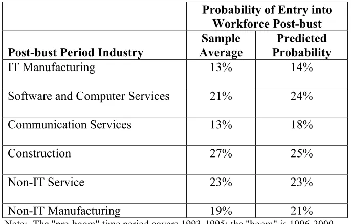
A test of the validity of this conclusion was performed by looking at entry into the
Georgia workforce during the post-bust period across industries. A probit estimation
identical to that described by equation (1) was estimated but with the sample conditioned
on being employed in Georgia during the post-bust period and entry being defined as
having been absent from the Georgia wage files prior to the post-bust period. If, indeed,
workers in the Software and Computer Services industry were motivated to enter the
Georgia workforce because of the employment and earnings opportunities available
during the IT boom, it is not expected that these workers should be entering the
since opportunities for IT workers were lower during the post-bust. Table 3 presents the
results from this probit estimation.
[Table 3 here]
The predicted probabilities in Table 3 indicate that IT workers (including those in
Software and Computer Services) were not any more likely to enter the Georgia
workforce during the post-bust period than workers in other industries.14 This is further
evidence that boom-period entrants into IT-industries were responding to the unique
economic opportunities of the time period.
VI. Conclusions and Implications
The IT boom pulled workers into Georgia’s IT sector, specifically the Software
and Computer Services industry, at higher rates than seen in other industries. However,
the decline of employment in the IT sector did not result in an analogous
disproportionately large push of those individuals out of the Georgia workforce. Given
that workers in the Software and Computer Services industry are among the highest paid
and most skilled in the workforce, the large inflow followed by the much smaller outflow
suggests that the IT boom in Georgia resulted in a net gain of skilled individuals in the
workforce. Thus, the IT boom resulted in Georgia’s workforce becoming more highly
concentrated with high-skilled workers.
An interpretation of this finding is that the inter-industry transferability of skills
for these workers allowed them to remain in the local workforce during economic
downturns. This is especially relevant in the case of workers at IT-service providing
decline in demand for workers with IT skills. Businesses outside of the IT sector brought
more IT services in-house during the IT bust, and this generated demand and employment
opportunities for IT workers leaving the IT sector. This is supported by the result that
nearly one third of workers who left the IT sector during the bust period transitioned into
non-IT Professional and Business Services Industries.
The results in this paper imply that economic development strategies that
encourage the growth of a highly educated workforce with skills that are transferable
across industries will result in a more resilient workforce. In other words, those regions
that focused on developing IT industries with larger concentrations of semi-skilled and/or
low-skilled workers, such as certain types of IT manufacturing, likely fared relatively
worse after the end of the IT-boom.15 In addition, there is some evidence that the
presence of high skilled (educated) workers helps a local economy to mitigate the effects
of negative economic shocks (Glaeser and Saiz, 2003). Furthermore, Giannetti (2001)
found that once a workforce has a large enough concentration of high-skilled workers, the
workers themselves benefit from the rents generated by skill complimentarity, thus
attracting more high-skilled workers. Thus, the results in this paper suggest that
development efforts to attract high skilled workers (or industries that employ skilled
workers) can have benefits that last beyond the life of the initial attraction.
There are several important considerations in trying to apply the experience
identified for Georgia to economic development planning and policy in other locales.
First is that Atlanta (the primary IT center of Georgia) enjoyed some unique natural
advantages in attracting skilled workers during the IT boom. One advantage was the
significant IT center in the nineties was Washington, D.C. That means that there was
very little competition in attracting high-skilled workers over a significant geographic
area. Other advantages include community and social characteristics that come together
to define a location's "quality of place" (see Florida, 2007 and Nucci et al., 2002) as well
as human capital, financial, and economic characteristics that define a location's
"knowledge competitiveness" (see Huggins and Izushi, 2007 and Partridge, 1993).
The second consideration is that the rapid growth of the IT sector in Georgia
during the 1990s was not a random event, but was associated with a concerted, diverse
effort by state and local governments, often in partnership with private enterprises, to
position the region as a major IT center. The primary example of these initiatives is the
Advanced Technology Development Center (ATDC) at the Georgia Institute of
Technology, which was created in 1980 to help establish links between research
institutions and the IT businesses.16 This very early effort of the ATDC created an
environment and made resources available to establish a critical mass of activity that
attracted skilled workers to the state, and was likely the reason why the IT specialization
in Atlanta became IT services, as opposed to IT hardware development (see Cortright and
References
Abraham, K. G., & Farber, H. S. (1987). Job duration, seniority, and earnings. American
Economic Review,77 (3), 278-97.
Barrow, L. (2004). Is the official unemployment rate misleading? A look at labor market
statistics over the business cycle. Federal Reserve Bank of Chicago Economic
Perspectives2 (2), 21-35.
Becker, G. (1964). Human Capital. New York: National Bureau of Economic Research.
Blevins, A. L., Jr. (1969). Migration rates in twelve southern metropolitan areas: a
"push-pull" analysis. Social Science Quarterly,50, 337-53.
Bowles, R. (2004). Employment and wage outcomes for North Carolina's high-tech
workers. Monthly Labor Review127 (5), 31-9.
Boyd, R. L. (2002). A 'migration of despair': unemployment, the search for work and
migration to farms during the great depression. Social Science Quarterly,83 (2),
554-67.
Bureau of Labor Statistics (2003, September 30). New quarterly data on business
employment dynamics from the BLS. Retrieved December 12, 2007, from
http://www.bls.gov/news.release/archives/cewbd_09302003.pdf
Bureau of Labor Statistics (2007). Career guide to industries (CGI), 2006-2007 edition.
Retrieved December 12, 2007 from http://www.bls.gov/oco/cg/home.htm.
Chiquiar, D., & Gordon H. H. (2005). International migration, self-selection, and the
distribution of wages: evidence from Mexico and the United States. Journal of
Daly, M., & R.G. Valetta. (2004). Performance of urban information technology centers:
the boom, the bust, and the future. Federal Reserve Bank of San Francisco
Economic Review, 1-18.
Dardia, M., Grose, T., Roghmann, H., & O'Brian-Strain, P. (2005). The high-tech
downturn in Silicon Valley: what happened to all those skilled workers?
Bulingame, CA: The SPHERE Institute.
DeBacker, J., Hotchkiss J., Pitts M., & Robertson J. (2005). It's who you are and what
you do: explaining the IT industry wage premium. Federal Reserve Bank of
Atlanta Economic Review, 90 (Q3) 37-45.
Economics and Statistics Administration. (2003). Digital economy 2003. Washington,
D.C.: U.S. Department of Commerce.
Fallick, B. D., & Fleischman, C.A. (2001). The importance of employer-to-employer
flows in the U.S. labor market. (Finance and Economics Discussion Series No.
2001-18).Washington D.C.: Federal Reserve Board of Governors.
Feliciano, C. (2005). "Educational selectivity in U.S. immigration: how do immigrants
compare to those left behind?" Demography,42 (1), 131-52.
Florida, R. (2007, November). Quality of place & the new economy: positioning
Pittsburgh to compete. Strategic Report, Retrieved November 30, 2007, from
http://www.sustainablepittsburgh.org/NewFrontPage/PublicDocs/Quality_of_Plac
e_Report.htm
Gabriel, P. E. and Schmitz, S. (1995). Favorable self-selection and the internal migration
of young white males in the United States. Journal of Human Resources,30 (3),
Giannetti, M. (2001). Skill complementarities and migration decisions." Labour,15,
1-31.
Glaeser, E. L. and Saiz, A. (2003). The rise of the skilled city. (Working Paper #10191).
New York: National Bureau of Economics Research, Center for Economics
Analysis.
Greenwood, M. (1975). Research on internal migration in the United States: a survey.
Journal of Economic Literatur, 13 (2), 397-433.
Greenwood, M. J. (1985). Human migration: theory, models and empirical studies.
Journal of Regional Science,25 (4), 521-44.
Haltiwanger, J., Lane J., Spletzer J., Theeuwes J., & Troske K. (1999). The creation and
analysis of employer-employee matched data. Amsterdam: North Holland.
Hotchkiss, J. L., Pitts M. M., & Robertson J.C. (2006). Earnings on the information
technology roller coaster: insight from matched employer-employee data."
Southern Economic Journal,73(2), 342-61.
Huggins, R. and Izushi H. (2007). The knowledge competitiveness of regional
economies: conceptualisation and measurement. Bank of Valletta Review, 35,
1-24.
Hunt, G. L. (1993). Equilibrium and disequilibrium migration modeling. Regional
Studies,27 (4), 341-49.
Kyriakoudes, L. M. (2003). The social origins of the urban South: race, gender, and
migration in Nashville and middle Tennessee, 1890-1930. Chapel Hill and
Light, A. (2005). Job mobility and wage growth: evidence from the NLSY79. Monthly
Labor Review, 128 (2), 33-9.
Long, C. D. (1958). The labor force under changing income and employment. Princeton,
NJ: Princeton University Press.
Mincer, J., & JovanovicB. (1981). Labor mobility and wages. In S. Rosen (Eds.), Studies
in labor markets (pp. 21-64). Chicago, IL: University of Chicago Press.
Nucci, A., Tolbert C., & Irwin M. (2002). Leaving home: modeling the effect of civic and
economic structure on individual migration patterns. (Working Paper No.
02-16). Washington D.C.: U.S. Census Bureau, Center for Economic Studies.
Partridge, M. (1993). High-tech employment and state economic development policies.
Review of Regional Studies, 23, 287-305.
Perrins, G. (2004). Employment in the information sector in March 2004. Monthly Labor
Review, 127 (9), 42-7.
Schafft, K. (2005, May). Poverty, residential mobility and student transiency within a
rural New York school district. Paper presented at Northeastern US Rural
Poverty Conference, Pennsylvania State University, University Park, PA.
Schultz, T. W. (1961). Investment in human capital. American Economic Review, 51,
1-17.
Schwartz, A. (1973). Interpreting the effect of distance on migration. Journal of Political
Economy, 81, 1153-67.
Thornthwaite, C. W. (1936). Internal migration in the United States. Philadelphia:
Todd, P. E., & Wolpin K.I. )2003). On the specification and estimation of the production
function for cognitive achievement. The Economic Journal, 113, F3-33.
White, S. B., Zipp J.F., McMahon W.F., Reynolds P.D., Osterman J.D., & Binkley L. S.
(1990). ES202: The data base for local employment analysis. Economic
Development Quarterly, 4, 240-53.
Zimmerman, K. F. (1996). European migration: push and pull. International Regional
Science Review, 19, 95-128.
Zoghi, C., & Pabilonia S.W. (2004). Which workers gain from computer use? (Working
Table 1. Sample means.
Mean (std. dev.)
Percent of workers absent from Georgia workforce pre-boom 26%
Workers in IT Manufacturing during boom 21%
Workers in Software and Computer Services during boom 34%
Workers in Communication Services during boom 23%
Workers in Construction during boom 31%
Workers in Non-IT Services during boom 27%
Workers in Non-IT Manufacturing during boom 21%
Percent of workers absent from Georgia workforce post-bust 31%
Workers in IT Manufacturing during boom 27%
Workers in Software and Computer Services during boom 31%
Workers in Communication Services during boom 28%
Workers in Construction during boom 37%
Workers in Non-IT Services during boom 31%
Workers in Non-IT Manufacturing during boom 28%
Percent of workers employed during the boom:
In IT Manufacturing 0.8%
In Software and Computer Services 3.5%
In Communication Services 2.3%
In Construction 7.6%
In Non-IT Services 65.5%
In Non-IT Manufacturing 20.4%
Total number of quarters during the boom with Interior Earnings 9.73
(6.52)
Job change rate 0.3045
(0.2987)
Average quarterly earnings during the boom $8,993
(6,798)
IT Manufacturing $11,666
(7,879)
Software and Computer Services $15,478
(9,310)
Communication Services $14,109
(7,470)
Construction $8,356
(4,927)
Non-IT Services $8,619
(6,820)
Non-IT Manufacturing $8,632
(5,794) Sample size = 3,150,731
Table 2. Predicted probability of entering and exiting Georgia's workforce by boom period industry.
Probability of Entry Probability of Exit
Boom Period Industry
Sample Average
Predicted Probability
Sample Average
Predicted Probability
IT Manufacturing 21% 22% 27% 28%
Software and Computer Services 34% 33% 31% 30%
Communication Services 23% 27% 28% 27%
Construction 31% 27% 37% 34%
Non-IT Service 27% 27% 31% 30%
Non-IT Manufacturing 21% 23% 28% 31%
Table 3. Predicted probability of entering Georgia's workforce during the post-bust period by post-bust period industry.
Probability of Entry into Workforce Post-bust
Post-bust Period Industry
Sample Average
Predicted Probability
IT Manufacturing 13% 14%
Software and Computer Services 21% 24%
Communication Services 13% 18%
Construction 27% 25%
Non-IT Service 23% 23%
Non-IT Manufacturing 19% 21%
Figure 1: U.S. IT-Sector Output and Employment 90 95 100 105 110 115 120 125 130 135 140 145 150 155
1993 1994 1995 1996 1997 1998 1999 2000 2001 2002 2003 2004 2005
Years E mp loym ent Ind ex ( 19 93 = 10 0) -15 -10 -5 0 5 10 15 O u tp u t %y/y
IT Employment Index (rhs) Non-IT Employment Index (rhs) IT-sector Output ($b)
Appendix A: Probit Estimation of Entering and Exiting the Georgia Workforce
Prob(Entering) Prob(Exiting) Coef
(std. error)
Coef (std. error)
Absent from Georgia Workforce Pre-Boom = 1 -- 0.2611
(0.0017)
Job change rate 1.4030
(0.0027) [0.4150]
0.9591 (0.0027) [0.3169]
Log Average Quarterly Earnings during the boom 0.0626
(0.0035) [0.0185] 0.0631 (0.0033) [0.0209] Boom Industry
IT Manufacturing = 1 -2.7459
(0.1523)
-1.2700 (0.1437)
Software and Computer Services = 1 -0.5274
(0.0726)
-0.0984ns (0.0719)
Communication Services = 1 1.3689
(0.1019)
-1.6319 (0.0979)
Construction = 1 0.4434
(0.0615)
0.9587 (0.0589)
Non-IT Services = 1 -0.2387
(0.0344)
-0.5698 (0.0323) Interaction Terms
Log Ave. boom Earnings * IT Manufacturing 0.3030
(0.0165) [0.1082]
0.1338 (0.0156) [0.0651]
Log Ave. boom Earnings * Software and Computer Services 0.0936
(0.0077) [0.0462]
0.0075ns (0.0076) [0.0233]
Log Ave. boom Earnings * Communication Services -0.1387
(0.0109) [-0.0225]
0.1694 (0.0104) [0.0768]
Log Ave. boom Earnings * Construction -0.0336
(0.0069) [0.0086]
-0.00989 (0.0066) [-0.0118]
Log Ave. boom Earnings * Non-IT Services 0.0406
(0.0039) [0.0305]
0.0614 (0.0036) [0.0411]
Constant -1.7671
(0.0315)
-1.4416 (0.0293) Sample size = 3,150,731
Appendix B: Percent of Workers That Did Not Exit Georgia and Were Not Employed in Their IT Boom Sector
Boom Period Employment
Post-bust Industry
Software and Computer Services
IT Manufacturing Communication Services
Construction 3.11 2.73 4.77
Manufacturing 6.45 19.05 7.82
Transportation & Utilities
3.31 3.52 3.27
Wholesale Trade 10.57 11.00 8.53
Retail Trade 8.42 10.08 13.47
Financial 15.65 3.83 9.06
Information 9.64 7.42 9.65
Professional & Business Services
31.01 31.25 30.43
Education and Health Services
6.99 6.30 7.17
Leisure & Hospitality 3.22 2.93 3.62
Public Administration 0 0 0
Other Services 1.63 1.89 2.21
Endnotes
1
One of the earliest treatments was Thornthwaite (1934). Also see Blevins (1969), Zimmermann (1996), Boyd (2002), and Kyriakoudes (2003).
2
An exception among the rural poor is found in Schafft (2005).
3
White et al. (1990) provide an extensive discussion about the use of these employment data, commonly referred to as the ES202 file. These are the UI data being used by the BLS to construct the Business Employment Dynamics data file introduced at a BLS briefing 30 September 2003 (Bureau of Labor Statistics 2003). These data are also now referred to as the Quarterly Census of Employment and Wages by the BLS (see www.bls.gov/cew).
4
Included in wages are pay for vacation and other paid leave, bonuses, stock options, tips, the cash value of meals and lodging, and in some states, contributions to deferred compensation plans (such as 401(k) plans). Covered employer contributions for old-age, survivors, and disability insurance (OASDI), health insurance, unemployment insurance, workers' compensation, and private pension and welfare funds are not reported as wages. Employee contributions for the same purposes, however, as well as money withheld for income taxes, union dues, and so forth, are reported even though they are deducted from the worker's gross pay.
5
See Haltiwanger et al. (1999) for a collection of studies using these and other employer-employee matched data sets. These state administrative data have also been used to investigate employment and earnings among IT workers in California (Dardia et al. 2005) and North Carolina (Bowles 2004). Also see Perrins (2004).
6
The classifications are based on those used in the Department of Commerce Report: Digital Economy 2003, with two modifications: Computer Training Schools are added to the Software and Computer Services category, and Computer Software Wholesalers and Retailers are included in Software and Computer Services instead of Computer Hardware.
7
Collapsing the long panel into a cross-section of observations is primarily done to allow identification of a worker's industry during the boom period. There are other strategies to do this. For example, one could be identified as an IT worker during the boom if employed in that sector for at least one quarter or in that sector for all quarters during the time period. These options are clearly the extremes, and don't solve the problem of what to do with someone employed in multiple industries across the period. The construction of a worker's modal activity and model industry provides a reasonable approach to identifying the industry that best describes a workers' industry association during the IT boom period.
8
This cut-off value was used in a study of Californian IT employment (Dardia et al. 2005). To also maintain the focus on a more "typical" IT worker, any worker whose earnings were top-coded at $100,000 per quarter was also eliminated. The earnings of 99 percent of workers fell well below this cap in every year.
9
The "full-time" restriction applied in the boom time period is not enforced for identifying workers who were employed during the pre-boom and post-boom time periods.
10
To the extent that physical migration is less costly for workers with more education (e.g., they have greater access to information), then more educated workers will exhibit greater tendency to migrate. For example, see Feliciano (2005) and Chiquiar and Hanson (2005).
11
The use of observed earnings to control for unobserved human capital characteristics is referred to as taking a value-added approach to measuring human capital (Todd and Wolpin 2003). See Zoghi et al. (2004) for another labor market application of this methodology.
12
These rates of turnover are consistent with those found in the literature. Abraham and Farber (1987) found that professional workers stay with the same employer for three years on average and blue-collar workers stay an average of two years; Light (2005) found that the average young worker changes employers about every two years, and Fallick and Fleischman (2001) also found the highest job change rate among construction workers and the lowest rate in manufacturing.
13
Alternative, less stringent, definitions of entry and exit were investigated, with no appreciable difference in the conclusions presented here.
14
The magnitudes of the percentages in Table 3 are not directly comparable to those in Table 2, since these two analyses are conditioning on employment and defining entry over periods of time of different lengths. However, comparing relative differences across industries is valid.
15
A test of that specific implication is beyond the scope of this paper, but matched employer-employee data of the type used in the current analysis would be well suited to addressing that question.
16