Changes in the dynamic relation between the prices and the trading volume from the Bucharest stock exchange

(1)

Munich Personal RePEc Archive

Changes in the dynamic relation between

the prices and the trading volume from

the Bucharest stock exchange

Dumitriu, Ramona and Stefanescu, Razvan and Nistor,

Costel

Dunarea de Jos University of Galati, Dunarea de Jos University of

Galati, Dunarea de Jos University of Galati

20 March 2011

Online at

https://mpra.ub.uni-muenchen.de/41602/

(2)

CHANGES IN THE DYNAMIC RELATION BETWEEN THE PRICES AND THE TRADING VOLUME FROM THE BUCHAREST STOCK EXCHANGE

RAMONA Dumitriu1, RAZVAN Stefanescu2, COSTEL Nistor3

1

Faculty of Economics and Business Administration/Department of Business Administration,University “Dunarea de Jos”,Galati, Romania,[email protected]

2

Faculty of Economics and Business Administration/Department of Economics,University “Dunarea de Jos”, Galati, Romania,[email protected]

3

Faculty of Economics and Business Administration/Department of Economics,University “Dunarea de Jos”, Galati, Romania,[email protected]

Abstract: This paper explores the relation between the prices and the trading volume from the Bucharest Stock Exchange. The data employed consist in the daily values from January 2002 to March 2011. We identify some significant changes caused by events such as Romania’s adhesion to the European Union or the effects of the global crisis.

Key words: Romanian StockExchange, Stock Index Volume, Trading Volume Causality

JEL classification: G 10, G 15

1. Introduction

The relation between the stock prices and the trading volume is one of the main topics of the financial economics. The study of interactions between these variables could reveal some mechanisms of the stock markets (Karpoff, 1987). In the last decades several scientific papers approached this subject. Many of them found a positive correlation between the stock returns and the trading volume (Rogalski, 1978; Karpoff, 1987; Gallant et al, 1992; Lee and Rui, 2002). The Granger causality method was largely used to analyze the nature of the relation between the prices and the trading volume, with different results. Hiemstra and Jones (1993) identified bidirectional causality between the stock returns and the trading volume, while Saatcioglu and Starks (1998) obtained various results in their study about six Latin American stock markets.

Some studies found an asymmetrical nature of the relation between the prices and the trading volume (Epps and Epps, 1976; Karpoff, 1987). Other articles revealed some particularities of these interactions in the context of emerging markets (Saatcioglu and Starks, 1998; Kamath and Wang, 2006; Kamath, 2007). It was also revealed the relation between the prices and the trading volume could suffer changes in time due to economic and political events (Sidra et al, 2009; Khan and Ahmed, 2009).

In this paper we analyze the changes that occurred in the relation between the prices and the trading volume from the Bucharest Stock Exchange (BSE). Founded in 1882, BSE was closed during the communist regime. In 1995 BSE was reopened. However, between 1997 and 2001 the difficulties of transition and the impact of the East Asian Financial Crisis caused a significant decline of the stock prices. After the consolidation of the national economy BSE experienced a recovery in 2001. Romania’s adhesion to the European Union in 2007 contributed to significant inflows of foreign capitals on the domestic stock market. In 2008 the impact of the global crisis caused another drastic decline. Since 2009 the stock prices increased again but the Romanian financial markets were still under threat of the new shocks from the national economy or from abroad.

In order to identify the differences between the corporations and the small companies we study the two main segments of BSE: BET and RASDAQ. While on BET there are listed the biggest Romanian companies, RASDAQ contained rather smaller companies. We analyze the price – volume trading relation during four periods:

- a first period, from January 2002 to December 2006, when BSE was stimulated by the consolidation of the national economy;

- a second period, from January to December 2007, when significant inflows of the foreign capitals occurred;

(3)

[image:3.612.102.522.114.458.2]

- a fourth period, from March 2010 to March 2011 when, despite a recovery, the threats of the new shocks persisted.

Figure 1: Evolution of the indices from the BET market (BETC) and from RASDAQ (RAQC) between January 2002 and March 2011

Source of data: BSE

In the next section there are described the data and the methodology employed in this paper. The third section presents the empirical results and the fourth section concludes.

2. Data and Methodology

In our investigation we use daily data of the trading volume and the closing index prices of the two main components of BSE: BET and RASDAQ. These values cover a period of time from January 2002 to March 2011. We split this sample of data into four sub-samples corresponding to the four phases mentioned before. We use two indices: BET-C for BET market and RAQ-C for RASDAQ market.

The returns of the two indices are computed using the equation:

Rt = ln (Pt) – ln (Pt-1) (1) where:

- Rt is the return on the day t;

- Pt is the closing market index price on the day t.

We also use detrended values of trading volume obtained as residuals of the regression equations.

We analyze the stationarity of the returns and of the detrended trading volume using the Augmented Dickey Fuller (ADF) test.

We employ two types of regressions to analyse the relation between the prices and the volume.

In the first equation the detrended values of the trading volume (Vt) represent the dependent variable, while the returns compose the independent one:

(4)

The second equation describes the dependence of the detrended values of the trading volume by the absolute values of the returns:

Vt = + abs (Rt) + t (3)

We also investigate the interactions and causalities between the two variables using Vector Autoregression (VAR) models (the number of lags is chosen based on the Akaike Information Criterion) and the Granger causality method.

3. Empirical Results

[image:4.612.70.543.241.485.2]

The descriptive statistics of BET and RASDAQ returns are presented in the Table 1. The means of BET returns are negative for the third sub sample, while the means of RASDAQ returns are negative for the third and fourth sub samples. The highest volatility, measured by the standard deviation, occurred in the third sub sample. For all the sub samples the skewness is negative, while the kurtosis exceeds the normal value. The Jarque-Bera tests indicate that all the time series are not normally distributed.

Table 1: Descriptive Statistics for Returns Indicator Mean Std. Dev. Skewness Ex. kurtosis

Jarque-Bera test

p-value for Jarque-Bera test BET Returns

First Sub-sample

0.00188088 0.0126980 -0.416985 6.68844 2337.79 0.0000

Second Sub-sample

0.00113000 0.0129814 -0.295533 1.62679 31.2063 0.0000

Third Sub-sample

-0.0054978 0.0269849 -0.413382 3.62795 155.762 0.0000

Fourth Sub-sample

0.00154913 0.0185706 -0.366924 4.47750 451.189 0.0000

RASDAQ Returns First

Sub-sample

0.0008478 0.00796909 -0.348741 20.2458 21117.5 0.0000

0.00270147 0.0116866 0.174541 1.97247 41.7968 0.0000

-0.0031882 0.0241675 -0.967427 79.6733 71455.2 0.0000

-0.0002492 0.0118135 -8.86945 149.389 496013 0.0000

Source of data: BSE

In the Table 2 there are presented the descriptive statistics of the trading volume. The means were highest for the second sub-samples. For all the sub samples the skewness is positive and the kurtosis exceeds the normal value. According to the Jarque-Bera tests all the time series are not normally distributed.

Table 2: Descriptive Statistics for Trading Volume Indicator Mean Std. Dev. Skewness Ex.

kurtosis

Jarque-Bera test

p-value for Jarque-Bera test BET Trading Volume

First Sub-sample

41.9187 79.6776 17.5724 443.505 1.01935e+007 0.0000

56.9398 51.4133 3.91750 18.4965 4203.2 0.0000

51.3295 49.9390 5.32106 39.3897 18729 0.0000

55.7533 160.255 17.4009 343.899 2.61855e+006 0.0000

RASDAQ Trading Volume First

Sub-sample

[image:4.612.68.542.560.736.2]

(5)

17.2461 64.6072 12.0839 163.932 286020 0.0000

7.64525 15.9682 7.73734 67.8584 54497.5 0.0000

5.67661 9.97088 12.2527 206.979 952078 0.0000

Source of data: BSE

[image:5.612.68.542.57.130.2]

We analyzed the stationarity of the variable using the Augmented Dickey-Fuller Tests. For all the sub samples we used constants as deterministic terms, while the number of lags was chosen by the Akaike Information Criterion. The results of the unit root tests, reported in the Table 3, indicate that all the time series are stationary.

Table 3:Results of Augmented Dickey-Fuller Tests

Indicator First Sub-sample Second Sub-sample Third Sub-sample Fourth Sub-sample BET Returns

Number of lags 32 20 18 21

Test statistic -6.91655 -3.5014 -15.9087 -5.46401 Asymptotic p-value 5.549e-010 0.00798 2.053e-029 2.086e-006

RASDAQ Returns

Test statistic -5.46368 -3.04971 -15.8842 -21.9267 Asymptotic p-value 2.09e-006 0.03053 4.296e-028 4.73e-038

BET Detrended Volume

Test statistic -4.35426 -13.8382 -2.88843 -4.95802 Asymptotic p-value 1.443e-005 1.212e-024 0.04669 2.486e-005

RASDAQ Detrended Volume

Test statistic -35.1186 -3.86483 -6.13944 -21.7158 Asymptotic p-value 7.849e-022 0.002321 5.493e-008 4.56e-038 Source of data: BSE

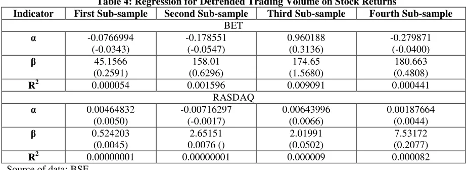
[image:5.612.69.532.498.666.2]

The regression results for the detrended trading volume on the stock returns are shown in the Table 4. We didn’t find any significant coefficient.

Table 4:Regression for Detrended Trading Volume on Stock Returns

Indicator First Sub-sample Second Sub-sample Third Sub-sample Fourth Sub-sample BET -0.0766994 (-0.0343) -0.178551 (-0.0547) 0.960188 (0.3136) -0.279871 (-0.0400) 45.1566 (0.2591) 158.01 (0.6296) 174.65 (1.5680) 180.663 (0.4808) R2 0.000054 0.001596 0.009091 0.000441

RASDAQ 0.00464832 (0.0050) -0.00716297 (-0.0017) 0.00643996 (0.0066) 0.00187664 (0.0044) 0.524203 (0.0045) 2.65151 0.0076 () 2.01991 (0.0502) 7.53172 (0.2077) R2 0.00000001 0.00000001 0.000009 0.000082 Source of data: BSE

(6)

Table 5: Regression for Detrended Trading Volume on Absolute Stock Returns

Indicator First Sub-sample Second Sub-sample Third Sub-sample Fourth Sub-sample BET -8.49568*** (-2.7768) -5.26057 (-1.0746) -8.70274** (-2.0938) -0.801775 (-0.0826) 952.849*** (3.9962) 539.665 (1.4336) 451.706*** (2.9875) 61.9167 (0.1188) R2 0.012786 0.008219 0.032229 0.000027

RASDAQ 0.457783 (0.3939) 4.62744 (0.7410) -0.0162523 (-0.0153) -0.229709 (-0.4652) -92.1837 (-0.6354) -510.318 (-0.9783) 1.64966 (0.0378) 38.9099 (0.9301) R2 0.000327 0.003844 0.000005 0.001648 Note: *** and ** indicate statistical significance at 0.01 and 0.05 per cent level respectively. Source of data: BSE

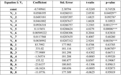
[image:6.612.104.523.329.588.2]

The results of the Vector Autoregression analysis for the BET market are shown in the Table 6. The interactions between the two variables are significant for the first and for the third sub-samples.

Table 6: Vector Autoregression analysis for the interactions between the Stock Returns and the Detrended Trading Volume from BET market

First sub - sample

Equation 1: Vt Coefficient Std. Error t-ratio p-value

const -0.749941 2.30794 -0.3249 0.74528 Vt _1 0.0588195 0.0286511 2.0530 0.04029**

Vt _2 0.0483181 0.0287207 1.6823 0.09276*

Vt _3 0.0461002 0.0287617 1.6028 0.10923

Vt _4 0.0926318 0.0286757 3.2303 0.00127***

Vt _5 0.115451 0.0286624 4.0279 0.00006***

Vt _6 0.00589222 0.0288306 0.2044 0.83810

Vt _7 0.0117568 0.0287635 0.4087 0.68280

Vt _8 0.0838992 0.0287312 2.9201 0.00356***

Rt _1 83.7992 177.985 0.4708 0.63785

Rt _2 331.02 181.116 1.8277 0.06785*

Rt _3 -77.9989 181.298 -0.4302 0.66711

Rt _4 -1.54574 181.208 -0.0085 0.99320

Rt _5 155.32 180.877 0.8587 0.39067

Rt _6 -23.6137 180.843 -0.1306 0.89613

Rt _7 -16.1624 180.656 -0.0895 0.92873

Rt _8 -11.0776 177.309 -0.0625 0.95019

Adjusted R-squared = 0.047676; F(16, 1210) = 4.836092; P-value(F) = 1.09e-09

Equation 2: Rt Coefficient Std. Error t-ratio p-value

const 0.00143625 0.00037234 3.8574 0.00012*** Vt _1 6.19733e-06 4.62229e-06 1.3407 0.18025

Vt _2 -4.42833e-06 4.63352e-06 -0.9557 0.33941

Vt _3 1.18263e-05 4.64012e-06 2.5487 0.01094**

Vt _4 1.488e-06 4.62625e-06 0.3216 0.74778

Vt _5 -4.51917e-06 4.6241e-06 -0.9773 0.32861

(7)

Vt _7 -7.84401e-06 4.64041e-06 -1.6904 0.09121*

Vt _8 1.34764e-06 4.6352e-06 0.2907 0.77130

Rt _1 0.223359 0.0287143 7.7787 0.00001***

Rt _2 -0.0341774 0.0292195 -1.1697 0.24236

Rt _3 0.0118758 0.0292488 0.4060 0.68480

Rt _4 -0.0743448 0.0292342 -2.5431 0.01111**

Rt _5 0.0237303 0.0291809 0.8132 0.41626

Rt _6 0.0207309 0.0291754 0.7106 0.47749

Rt _7 0.108838 0.0291452 3.7343 0.00020***

Rt _8 -0.0300223 0.0286053 -1.0495 0.29414

Adjusted R-squared = 0.063210; F(16, 1210) = 6.170282; P-value(F) = 2.45e-13 Source of data: BSE

Second sub – sample

const -0.231 3.21773 -0.0718 0.94283 Vt _1 0.123177 0.0636161 1.9363 0.05400*

Vt _2 0.0951049 0.0634751 1.4983 0.13535

Rt _1 -476.948 256.345 -1.8606 0.06401*

Rt _2 659.457 249.694 2.6411 0.00880***

Adjusted R-squared = 0.043427; F(16, 1210) = 3.803375; P-value(F) = 0.005097

const 0.00084265 0.000809163 1.0414 0.29873 Vt _1 1.70183e-05 1.59976e-05 1.0638 0.28847

Vt _2 3.52607e-06 1.59621e-05 0.2209 0.82535

Rt _1 0.0892814 0.0644633 1.3850 0.16732

Rt _2 0.0316713 0.0627906 0.5044 0.61444

Adjusted R-squared = -0.001592; F(16, 1210) = 0.901874; P-value(F) = 0.463482 Source of data: BSE

Third sub – sample

const 0.691672 3.04356 0.2273 0.82040 Vt _1 0.138305 0.0609176 2.2704 0.02400**

Vt _2 0.136881 0.0608042 2.2512 0.02521**

Vt _3 0.20266 0.0607578 3.3355 0.00098***

Rt _1 62.8801 107.904 0.5827 0.56057

Rt _2 120.32 108.396 1.1100 0.26803

Rt _3 -70.2858 108.265 -0.6492 0.51678

Adjusted R-squared = 0.100016; F(16, 1210) = 5.926800; P-value(F) = 8.10e-06

const -0.00537514 0.00174927 -3.0728 0.00235*** Vt _1 -3.21423e-06 3.5012e-05 -0.0918 0.92692

Vt _2 2.96084e-05 3.49469e-05 0.8472 0.39764

Vt _3 3.34914e-05 3.49202e-05 0.9591 0.33841

(8)

Rt _2 -0.0246311 0.0623001 -0.3954 0.69290

Rt _3 -0.0596896 0.0622245 -0.9593 0.33832

Adjusted R-squared =-0.001763; F(16, 1210) = 0.921982; P-value(F) = 0.479550 Source of data: BSE

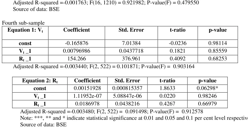
Fourth sub-sample

const -0.165876 7.01384 -0.0236 0.98114 Vt _1 0.00796986 0.0437718 0.1821 0.85559

Rt _1 154.266 376.961 0.4092 0.68253

Adjusted R-squared =-0.003440; F(2, 522) = 0.101871; P-value(F) = 0.903164

const 0.00151928 0.000815357 1.8633 0.06298* Vt _1 1.11952e-07 5.08847e-06 0.0220 0.98246

Rt _1 0.0186978 0.0438216 0.4267 0.66979

Note: ***, ** and * indicate statistical significance at 0.01 and 0.05 and 0.1 per cent level respectively. Source of data: BSE

[image:8.612.103.537.86.314.2]

In the Table 7 there are presented the results of Vector Autoregression analysis for the RASDAQ market. The interactions between the two variables are lowest for the fourth sub-sample.

Table 7: Vector Autoregression analysis for the interactions between the Stock Returns and the Detrended Trading Volume from RASDAQ market

First sub – sample

const -0.141736 0.934585 -0.1517 0.87948 Vt _1 0.00075181 0.0285706 0.0263 0.97901

Vt _2 -0.00352538 0.028521 -0.1236 0.90165

Vt _3 -0.000265825 0.0285227 -0.0093 0.99257

Rt _1 -21.6163 116.311 -0.1859 0.85259

Rt _2 251.292 118.246 2.1252 0.03377**

Rt _3 -49.5817 118.043 -0.4200 0.67454

Adjusted R-squared = -0.001160; F(16, 1210) = 0.762217; P-value(F) = 0.599724

const 0.000663922 0.000228817 2.9015 0.00378*** Vt _1 1.2622e-06 6.99502e-06 0.1804 0.85683

Vt _2 -2.65723e-06 6.98288e-06 -0.3805 0.70361

Vt _3 1.7441e-06 6.98329e-06 0.2498 0.80282

Rt _1 0.0907762 0.0284767 3.1877 0.00147***

Rt _2 0.0474058 0.0289504 1.6375 0.10179

Rt _3 0.0846101 0.0289008 2.9276 0.00348***

Adjusted R-squared =0.015586; F(16, 1210) = 4.248394; P-value(F) = 0.000304 Source of data: BSE

(9)

const 1.31598 4.24631 0.3099 0.75689 Vt _1 -0.000917082 0.0639417 -0.0143 0.98857

Vt _2 -0.0381102 0.06368 -0.5985 0.55009

Rt _1 -918.158 369.739 -2.4833 0.01369**

Rt _2 467.845 371.089 1.2607 0.20861

const 0.00177636 0.000723589 2.4549 0.01479 Vt _1 -1.6383e-05 1.08959e-05 -1.5036 0.13399

Vt _2 -2.7163e-05 1.08513e-05 -2.5032 0.01297**

Rt _1 0.224725 0.063005 3.5668 0.00044***

Rt _2 0.150585 0.0632351 2.3813 0.01802**

Adjusted R-squared =0.119067; F(16, 1210) =9.346159 ; P-value(F) = 4.84e-07 Source of data: BSE

Third sub – sample

const 0.0289976 0.985004 0.0294 0.97654 Vt _1 0.00237231 0.0613108 0.0387 0.96916

Rt _1 9.9068 40.4204 0.2451 0.80657

Adjusted R-squared = -0.007285; F(2, 266) = 0.030817; P-value(F) = 0.969656

Equation 2: Rt

Coefficient Std. Error t-ratio p-value

const -0.00304582 0.0013819 -2.2041 0.02838** Vt _1 0.00057427 8.60152e-05 6.6764 0.00001***

Rt _1 0.027223 0.0567073 0.4801 0.63158

Adjusted R-squared = 0.137785; F(2, 266) = 22.41362; P-value(F) = 1.01e-09 Source of data: BSE

Fourth sub – sample

const 0.0116348 0.428485 0.0272 0.97835 Vt _1 0.0513635 0.043689 1.1757 0.24027

Rt _1 28.0362 36.2673 0.7730 0.43985

Equation 2: Rt

Coefficient Std. Error t-ratio p-value

const -0.000264063 0.000515731 -0.5120 0.60885 Vt _1 4.12911e-05 5.25847e-05 0.7852 0.43267

Rt _1 0.0429428 0.0436518 0.9838 0.32569

(10)

[image:10.612.68.533.111.351.2]

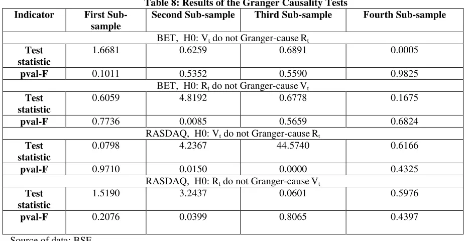
The results of the Granger Causality Tests are presented in the Table 8. For the second sub-sample, on the BET market returns Granger-cause volume, while for the RASDAQ market we found a bidirectional causality. For the third sub-sample, on the RASDAQ market volume Granger-cause returns.

Table 8: Results of the Granger Causality Tests Indicator First

Sub-sample

Second Sub-sample Third Sub-sample Fourth Sub-sample

BET, H0: Vt do not Granger-causeRt

Test statistic

1.6681 0.6259 0.6891 0.0005

pval-F 0.1011 0.5352 0.5590 0.9825 BET, H0: Rt do not Granger-causeVt

0.6059 4.8192 0.6778 0.1675

pval-F 0.7736 0.0085 0.5659 0.6824 RASDAQ, H0: Vt do not Granger-causeRt

0.0798 4.2367 44.5740 0.6166

pval-F 0.9710 0.0150 0.0000 0.4325 RASDAQ, H0: Rt do not Granger-causeVt

1.5190 3.2437 0.0601 0.5976

pval-F 0.2076 0.0399 0.8065 0.4397

Source of data: BSE

3. Conclusions

This paper approached the changes occurred in the relation between the stock market returns and the trading volume from two main components of BSE: BET and RASDAQ. We found significant differences between these segments that could be considered as a reflection of the size impact on this relation. We also identify an asymmetrical behavior on the BET market for the first and the third sub-sample, when the returns experienced the highest, respectively the lowest means.

On the BET market the results showed that returns Granger caused the volume only for the second sub-sample. In this period of time the significant inflows of the foreign capital encouraged the speculative transactions. In these circumstances the information contained in evolution of the returns influenced the volume of transactions. For the same period of time on the RASDAQ market we found bidirectional causality, suggesting that in comparison with the BET market the returns were more sensitive to the trading volume.

For the third sub-sample on the RASDAQ market the trading volume Granger caused the returns. In this period of time the financial markets were affected by the global crisis and the investors from the RASDAQ market, considered riskier than the BET markets, were very sensitive to the evolution of the trading volume.

4. References

• Campbell, J.; Grossman, S.; Wang, J. (1993) Trading Volume and Serial Correlation in Stock Returns, Quarterly Journal of Economics, Vol. 108, p. 905-939.

• Chen, G. M.; Rui, O. M.; Wang, S.S. (2005) The Effectiveness of Price Limits and Stock Characteristics: Evidence from the Shanghai and Shenzhen Stock Exchanges, Review of Quantitative Finance and Accounting, Vol. 25, p. 159-182.

(11)

• Epps, T.; Epps, M. (1976) The Stochastic Dependence of Security Price Changes and Transaction Volumes: Implications for the Mixture-of-Distributions Hypothesis, Econometrica, Vol. 44, p. 305-321.

• Gallant, R.; Rossi, P.; Tauchen, G. (1992) Stock prices and volume, Review of Financial Studies, Vol.5, p. 199-242.

• Granger, C. (1969) Investigating Causal Relations by Econometric Models and Cross-Spectral Methods, Econometrica, Vol. 37, 424-438.

• Hiemstra, C.; Jones, J.D. (1994) Testing for linear and nonlinear Granger causality in the stock price - volume relation, Journal of Finance 49 (5): p. 1639-1664.

• Kamath, R.; Wang, Y. (2006) The Causality between Stock Index Returns and Volumes in the Asian Equity Markets, Journal of International Business Research, Vol.5, p. 63-74.

•

Kamath, R. (2007) Investigating Causal Relations Between Price Changes and Trading

Volume Changes in the Turkish Market,

ASBBS E-Journal

, Volume 3, No. 1.

•

Kamath, R. (2008) The Price-Volume Relationship in the Chilean Stock Market,

International Business & Economics Research Journal

– October, Volume 7, Number 10.

• Karpoff, J.M. (1987) The relation between price changes and trading volume: A survey, Journal of Financial and Quantitative Analysis, 22 (1): p. 109-126.

• Khan, A.; Ahmed, S. (2009) Trading Volume and Stock Return: The Impact of Events in Pakistan on KSE 100 Indexes, International Review of Business Research Papers, Vol. 5 No. 5, September, p. 373-383.

• Lee, B-S; Rui, O.M. (2002) The dynamic relationship between stock returns and trading volume: Domestic and cross-country evidence, Journal of Banking and Finance, 26 (1): p. 51- 78.

• Medeiros, O.; Van Doornik, B. (2008) The Empirical Relationship between Stock Returns, Return Volatility and Trading Volume in the Brazilian Stock Market, Brazilian Business Review, Vol. 5, No. 1, Ian - Apr, p. 1-17.

• Rogalski, R. J. (1978), The Dependence of Prices and Volume, Review of Economics and Statistics, Vol. 60, p. 268-274.

• Saatcioglu, K.; Starks, L. T. (1998) The stock price-volume relationship in emerging stock markets: The case of Latin America, International Journal of Forecasting, 14, p. 215–225.

• Sidra, M.; Shahid, H.; Shakil, A. (2009) Impact of Political Event on Trading volume and Stock Returns: The Case of KSE, International Review of Business Research Papers,Vol. 5 No. 4, June, p. 354-364.

• Smirlock, M.; Starks, L. T. (1985) A Further Examination of Stock Price Changes and Transactions Volume, Journal of Financial Research, 8(3), p. 217-225.

• Smirlock, M.; Starks, L. T. (1988) An Empirical Analysis of the Stock Price-Volume Relationship,