NBER WORKING PAPER SERIES
ON ESTIMATING THE EXPECTED RETURN ON THE MARKET: AN EXPLORATORY INVESTIGATION
Robert C. Merton
Working Paper No.
444
NATIONAL BUREAU OF ECONOMIC RESEARCH 1050 Massachusetts Avenue
Cambridge MA 02138 February 1980
The research reported here is part of the NBER's research project on Debt and Equity. Any opinions expressed are those of the author and not those of the National Bureau of Economic Research.
On Estimating the Expected Return on the Market: An Exploratory Investigation
ABSTRACT
The expected return on the market is a number frequently required for the solution of many investment and corporate finance problems. However, by comparison with other financial variables, there has been relatively little academic research on estimating this expected return. The current practice for estimating the expected return on the market is to take the historical average of realized excess returns on the market and add, :It to'the current observed inte're~t: rate. While th;i:smodel does explicitly relfect the depen-dence of the market experience return ,on the interest rate, it does not take into account the effect of changes in the level of risk associated with the market.
Three models of equilibrium expected market returns which do reflect this dependence are analyzed in this paper. Estimation procedures are derived which incorporate the prior restriction that equilibrium expected excess returns on the market must be positive. The parameters of the models are estimated using realized return data for the period 1926-1978.
The principal conclusions from this exploratory investigation are:
~irst, in estimating models of the expected return on the market, the
non-negativity restriction of the expected excess return should be explicitly included as part of the specification. Second, estimators which use realized return time series should be adjusted for heteroscadasticity.
Robert C. Merton
Department of Economics
Massachusetts Institute of Technology Bldg. E52, Room 243
Cambridge, Massachusetts 02139 (617) 253-6617
ON ESTIMATING THE EXPECTED RETURN ON THE MARKET:
An Exploratory Inv~stigation
Robert C. Merton*
Massachusetts Institute of Technology
I. Introduction
Modern finance theory has provided many insights into how security prices are formed and has provided a quantitative description for the risk structure of equilibrium expected returns. In the most basic form of the Capital Asset Pricing Model,ll this equilibrium structure is given by the Security Market Line relationship: Namely,
ai - r •
a
i (a - r) (1.1)where a
i and a denotes the expected rate of return on security i and the market portfolio, respectively; r is the riskless interest rate; and
a
i is the ratio of the covariance of the return on security i with the return on the market divided by variance of the return on the market. ,This same basic model tells us t~at all efficient or optimal portfolioscan be represented by a simple combination of the market portfolio with the riskless asset. Hence, if ae and cre are the expected rate of return and standard deviation of return on an efficient portfolio, then ae
=
w(a - r)+
rand cre=
we where w· is the fraction allocated to the market and cr is the standard deviation of the return on themarket. From these conditions, we have that the equilibrium tradeoff between risk and return for efficient portfolios is given by
(1.2) is called the Capital Market Line and (a - r)/a, the slope of
that lin~is called the Price of Risk.
From (1.1) and (1.2), one can determine the optimal portfolio
allocation for an investor and the proper discount rate to employ for the evaluation of securities. Moreover, these equations provide the critical "cost of capital" or "hurdle rates" necessary for corporate capital
budgeting decisions. Of course, (1.1) and (1.2) apply only for the most basic version of the CAPM, and indeed, empirical tests of the Security Market Line have generally found that while there is a positive relation-ship between beta and average excess return, there are significant
deviations from the predicted relationship.!/ However, these deviations appear principally in very "high" and very "low" beta securities. MOreover, there is some question about the validity of these tests.3/ The more sophisticated intertemporal and arbitrage-model versions of the
. 4/
CAP~ show that equilibrium expected returns on securities may depend upon other types of risk in addition to "systematic" or "market" risk, 'arid hence, they provide a theoretical foundation for (1.1) and (1.2) not
to obtain. However, in all of these models, the market risk of
a security will affect its equilibrium expected return, and indeed, for
. 5/
most common stocks, market risk will be the dominant factor.-Thus, at least for common stocks and broad-based equity portfolios, the basic model as described by (1.1) and (1.2) should provide a reasonable "first approxi.Jnation" theory for equilibrium expected returns.
Of course, all one needs to know to apply these formulas in solving portfolio and corporate financial problems are the parameter values.
And as might be
-3-expected, considerable effort has been applied to estimating them. However, this effort has not been uniform with respect to the different parameters, and as will be shown, this nonuniformity is not without good reason.
For the most part, r is an observable, and so that parameter is gotten for free. Among the other parameters, beta is the one most widely estimated. In dozens of academic research papers, betas have been
estimated for individual stocks; portfolios of stocks; bonds and other fixed income securities; other investments such as real estate; and even human capital..§.! For practitioners, there are beta "books" and beta services. While for the most part these betas are estimated from
time series of past returns, various accounting data have also been used. In their pioneering work on the pricing of options and corporate liabilities, Black and Scholes (1973) deduced an option pricing formula whose only nonobservable input is the variance rate on the underlying stock.
As a result, there has been a surge in research effort to estimate the variance .. rates for returns on both individual stocks and the market. Although this
research activity is still in its early stages of development, variance rate estimates are already available from a number of sources.
In contrast, there has been little academic research on
estimating the expected return on either individual stocks or the market. Ibbotson and Sinquefield (1976; 1979) have carefully cataloged the
historical average returns on stocks and bonds from 1926 to 1978.
However, they provide no model as to how expected returns change through time. There is no literature analogous to the term structure of
interest rates for the expected return on stocks, although there is research going on in this direction as, fOr example, in Cox, Ingersoll, and Ross (forthcoming).
One possible explanation for this paucity of research on expected returns is that for many applications within
finance, only relative pricing relationships are used, and therefore, estimates of the expected returns are not required. Some important
examples of such applications are option and corporate liabilities pricing and the testing for superior performance of actively-managed portfolios. However, for many if not most applications, an estimate of the expected return on the market is essential. For example, to implement even the most passive strategy of portfolio allocation, an investor must know
the expected return on the market and its standard deviation in order to choose an optimal mix between the market portfolio and the riskless asset. Indeed,· even if one has superior security analysis skills so that the optimal portfolio is no longer a simple mix of the market and the riskless asset, TreynJr and Black (1973) have shown that the optimal strategy will still involve mixing the market portfolio with an active portfolio, and the optimal mix between the two will depend upon the expected return and standard deviation of the market. For a corporate finance example, the application of the model in determining a "fair" rate of return for investors in regulated industries requires not only the beta but also an estimate of the expected return on the market. As these examples
illustrate, it is not for want of applications that expected return estimation has not been pursued.
A more likely explanation is simply that estimating expected returns from time series of realized stock return data is very difficult. As is shown in Appendix A, the ·estimates of variances or covariances from the
-5-available time series will be much more accurate than the. corresponding expected return estimates. Indeed, even if the expected return on the market were known to be a constant for all time, it would take a very long history of returns to obtain an accurate estimate. And, of course, if
this expected return is believed to be changing through time, then estimating these changes is still more difficult. Further, by the
Efficient Market Hypothesis, the unanticipated part of the market return (i.e., the difference between the realized and expected return) should not be forecastab1e by any predetermined variables. Hence, unless a significant portion of the variance of the market returns is caused by changes in the expected return on the market, it will be difficult to use the time
series of realized market returns to distinguish among different models for expected return.
In light of these difficulties, one might say that to attempt to estimate the expected return on the market is to embark on a fool's errand. Perhaps, but on this errand, I present three models of expected .. return and derive methods for estimating them. I also report the results
of applying these methods to market data from 1926 fo 1978.
The paper is exploratory by design, and the empirical estimates presented should be viewed with that in mind. Its principal purpose is to motivate further research in this area by pointing out the many estima-tion problems and suggesting direcestima-tions for possibly solVing them. The reasons for taking this approach are many: First, an important input for estimating the expected return on the market is the variance rate on the market. While there is much research underway in developing variance
estimation models, their development has not yet reached the point where there is a "standard" model with well-understood error properties.
Because this is not a paper on variance estimation, the model used to estimate variance rates here is a very simple one. Almost certainly, these variance estimates contain substantial measurement errors, and these alone are enough to warrant labeling the derived model estimates for
expected return as "preliminary." A second reason is that the expected return model specifications are themselves very simple, and undoubtably could be improved upon. Third, only time series data of market returns were used in the estimations, and as is indicated in the analysis, other sources of data could be used to improve the estimates. As a reflection of the preliminary nature of this investigation, no significance tests are provided and no attempt is made to measure the relative forecasting
-7-II. The Models of Expected Return
The appropriate model for the expected return on the market will depend upon the information available. For example, in the absence of any other information, one might simply use the historical sample average of realized returns on the market. Of course, we do have other informa-tion. For example, we can observe the riskless interest rate. Noting that this rate has varied between essentially zero and its current doub1e-digit level during the last fifty years, we can reject the simple sample average model for two reasons: First, it can be proved as a rather general proposition that a necessary condition for equilibrium is that the expected return on the market must be greater than the riskless rate (i. e., a » r .
11
Hence, if the current interest rate exceeds the longhistorical average return on stocks (as it currently does), then the sample average is a biased-low estimate. Thus, one would expect the expected return on the market to depend upon the interest rate. Second,
the historical average is in nominal terms, and no sensible model would suggest .. that the equilibrium nominal expected return on the market is independent
of the rate of inflation which is also observable. Both these criticisms are handled by a second-level model which assumes that the expected excess return on the market, a - r, is constant. Using this model, the current
expected return on the market is estimated by taking the historical average excess return on the market and adding to it the current observed interest rate.
Indeed, a model of this type represents essentially the state-of-the-art with respect to estimating the expected return on. the market •.§.1
expected return on the interest rate and in so doing, it implicitly takes /-iuto account the level of inflation. However, it does not take into account another important determinant of market expected return: Namely, the level of risk associated with the market. At the extreme where the market is risk-less, -then by arbitrage, a.
=
r, and the risk premium on the market will be zero. If the market is not riskless, then the market mu~t have a positive risk9/
premium. While it need not always be the case,- a generally-reasonable assumption is that to induce risk-averse investors to bear more
risk, the expected return must be higher. Given tha~ in the aggregate, the market must be held, this assumption implies that, ceteris paribus, the equilibrium expected return on the market is an increasing function of the risk of the market. Of course, if changes in preferences or in the
distribution of wealth are such that aggregate risk aversion declines between one period and another, then higher market risk in the one
period need net imply a correspondingly higher risk premium. However, if aggregate risk aversion changes slowly through time by comparison with the changes in market risk, then, at least locally in time, one would
-expect higher levels of risk to induce a higher market risk premium. If, as shall be assumed, the variance of the market return is a
sufficient statistic for its risk, then a reasonably general specification of the equilibrium expected excess return can be written as
where g
2
a. -
r .. Yg(O' )is a function of 0'2 only, with g(O)" 0 and
(11.1) 2
dg/dO' >O. In the analysis to follow, we shall assume that the function g is
-9-known and that 02 can be observed. It is also assumed that there is a set of state variables S in addition to the current 02 that can be observed. The specific identity of these state variables will depend upon the data set available. However, Y is not one of these state variables. Hence, conditional on this information set, the expected excess return on the market is given by
(11.2)
where E[
Is,a
2] is the conditional expectation operator, conditional on knowing S ando •
2 Since Y is not observable, for (11.2) to have meaningful content, the further condition is imposed that(11.3)
That is, given the state variables S, the conditional expectation of Y does not depend upon the current
o .
2 This condition, of course, does not imply that Y. is independent ofrewrite (11.2) as
2
o . Thus, from (11.3), we can
(11.4)
Since it has already been assumed that variance is a sufficient statistic for risk, with little loss in generality, it is further assumed that
market returns can be described by a diffusion-type stochastic process in the context of a continuous-time dynamic mode1.101 Specifically, the instantaneous rate of return on the market (including dividends), dM/M, can be represented by the Ita-type stochastic differential equation
dM(t) • adt
+
odZ(t)M(t) (11.5)
,
.where dZ(t) is a standard Wiener process and (11.5) is to be inter-preted as a conditional equation at time t, conditional on the ins tan-taneous expected return on the market at time t, a(t)
=
a and on thein the context of instantaneous standard deviation of that return at time
d " d " " 11/" b 1
Un er certa~n con ~t10ns,-- ~t can e Slown
t, a(t)
=
a.
an intertemporal equilibrium mod~l that toe equilibrium instantaneous expected excess return on the market can be reasonably approximated by
(11.6)
where Yl is the reciprocal of the weighted sum of the reciprocal of each investor's relative risk aversion and the weights are related to the distri-bution of wealth among investors. To add further interpretation for Y
l, in the frequently-assumed case of a representative investor with a constant relative risk aversion utility function, Y
l would be an exact constant
and equal to this representative investor's relative risk aversion. The specifi-cation for expected excess return given by (11.6) which will be referred
to as "Model 111" is indicative of models where it is assumed that aggre-gate risk preferences remain relatively stable for appreciable periods of time.
"Model
In"
makes the alternative assumption that the slope of the Capital Market Line or the Market Price of Risk remains relatively stable for appreciable periods of time. Its specification is given by-11-where Y
2 is the Market Price of Risk. Like "Model 111," it allows for
cl,anges in the expected excess return as the risk level for the market changes. "Model #3" is the state-of-the-art model which assumes that the
expected excess return on the market remains relatively stable for appreciable periods of time even though the risk level of the market is changing. Its specification is given by
(11.8) Of course. if the variance rate on the market were to be essentially constant through time, then all three models would reduce to the state-of-the-art model with a constant expected excess return. However, from the work of Rosenberg (1972) and Black (1976) as well as many others, the hypothesis that the variance rate on the market remains constant over any appreciable period of time can be rejected at almost any confidence level. MOreover, given that the variance rate is changing, the three models are mutually exclu~ive in the sense that if one of the models satisfies condition (11.3), then the other two models cannot. To this, note that
_ j-i
Y
j - Yi[a(t}] for i,j
=
1,2,3. Therefore, if Yi satisfies (11.3), then E[Yjls]=
E[Yils]E{[a(t)]j-ils}. E[Yjls,a2(t)]=
E[Yils] [a(t)]j-i. Therefore, for i+
i, Yj can only satisfy (11.3) if
E{[aCt)]j-iI S}
=
[a(t)]i-i for all possible values of aCt), and this is not possible unless the {a(t)}· are constant over time.While we have assumed that
~(t)
is observable, in reality, it is not, and therefore; like aCt), it must be estimated. Hence, these models as special cases of (11.1) will be of empirical significance onlyif for the available data set, the variance rate can be estimated more accurately than the expected return. If the principal component of such a data set is the time series of realized market returns, then it is shown as a theoretical proposition in Appendix A that, indeed, the variance rate can be more accurately estimated when the market return
dynamics are given by (11.5). As an empirical proposition, the studies of both Rosenberg (1972) and Black (1976) show that a nontrivial portion
of the change in the variance can be forecasted by using even relatively simple models. Further, along the lines of Latane' and Rendleman (1976) and Schmalensee and Trippi (1978), it is possible to use observed option prices on stocks to deduce "ex-ante" market estimates for variance rates by "inverting" the Black-Scholes option pricing formula. Hence, models
of the type which satisfy (11.4) hold out the promise of better estimates for the expected return on the market than can be obtained by direct estimation from the realized market return series.
While (11.5) describes the dynamics of realized market returns, we have yet to specify how
aCt)
and Y.,J j
=
1,2,3 change through time. Although aCt) changes through time, it is assumed to be a slowly-varying function of time relative to the time scale of marketprice changes, and,'therefore, over short intervals of time,' the variation- in realized market returns will be very much larger than the variation in
the variance rate. That is, it is assumed that
for satisfactorily small 0, there exists a finite time interval h such that the probfla2(s) - a2(t)
I
> o!EI£(t,t+
h)} will be essentially zero where ,,2(t) "[1.'
,,2(s)dsl h . In essence, we assume that the variance
-13-rate can be treated as constant over finite time intervals of length h and that h» dt. In a similar fashion, it is also assumed that the riskless interest rate can be treated as constant over this same finite time interval h.
Under the hypothesis that Model
OJ
is the correct specification, we assume that Yj is a slowly-varying function of time relative to the time scale of changes in the variance rate. That is, there exists a finite time interval T, T» h, such that Y
j can be treated as essentially constant over intervals of that length. Again, because Y
j = yi[a(t)]j-i, i, j
=
1,2,3 if one of the models satisfies this assumption, then the other two cannot.It follows immediately from these hypothesized conditions and the model specifications that the expected rate of return on the market, aCt), can be treated as essentially constant over time intervals of
length h. Therefore, over short intervals of time, the variation in the expected return on market will be similar in magnitude to the variations .. in cr2(t) and r(t) and very much smaller than the variation in
realized market returns.
Let ~(t):: Met + h}!M(t) denote the return per dollar on the
market portfolio between time t and t + h. Under the hypothesized conditions for the dynamics of a(t) and Y
j , we have from (II.5) that conditional on knowing M(t), a(t), and ret), ~(t) will be lognormally
distributed. [t+h ]
Let R(t):: exp ~ r(s)ds denote the return per dollar on the riskless asset between t and t + h and define X(t) :: In[~(t)!R(t)].
Under the hypothesis that Model
OJ
is the correct specification~we can X(t) a;g./
e:..:press '"
(II. 9)
t+h
where Z(t;h) -
J(
dZ is a normally distributed random variable with mean equal to zero and a standard deviation equal to~. Moreover, for all t and t' such that It' - tl ~ h, Z(t;h) and Z(t';h) will be independent.In preparation for the model estimation, we proceed as follows: Let T denote the total length of time over which we have data. The first step is to partition the data into neT)(= T!T) nonoverlapping time periods of length T. By hypothesis, will be constant within each of these neT) time periods. The second step is to partition each of these neT) time periods into N(= T!h) nonoverlapping subperiods of length h. By hypothesis, the variance and interest rates will be
-constant within each of these N subperiods.
Since by hypothesis none of the variables relevant to the estimation changes during any of the nonoverlapping subperiods of length h, there is nothing to be gained by further subdivisions. Hence, the interval between observations will equal h, and by appropriate choice of time units, h can be set equal to one. Therefore, all time-dimensioned variables are expressed in units of the chosen observation interval.
Because within each of the neT) time periods, the subperiods are of identical length and nonoverlapping, it should cause no confusion to
-15-redefine the symbol "t" to mean "the ~th subperiod of length' h" within' a particular time period of length h. So redefined, t will take on integer values running from t
=
1, ••• ,N. There is no need to further distinguish "t" as to the time period in which it takes place because(a) the posited stochastic processes are time homogeneous; (b) the length of the subperiods are the same for all n(T) time periods; and (c) the
units,
neT)
"t"
time periods are nonoverlapping. By the choice for time th
will also denote the ~ observation within a particular time period.
With t redefined and h
=
1, (II.9) can be rewritten for a particular time period ast
=
1, ••• ,N (IL10)where g(t) is a standard normal random variable. Because the subperiods are nonoverlapping, g(t) and g(t') will be independent for all t and t' such that t ~ t'. For the N observations within this time period, Y
j is, by hypothesis, a constant.
With this, the descriptions of the models are complete, and we now turn to the development of the estimation procedures.
III. The Estimation Procedures
Given a time series of estimates for aCt), the natural estimation procedure suggested by (11.10) is least-squares regression. (11.10) is put in standard form, by making the change in variables X'{t)
=
x{t)!a(t)+
a{t)!2
and rewriting (11.10) for ModelOJ
as X'(t)=
Y [a{t)]2-j + E(t)j .
Given the
N
observations within the time period over which Y j'"
constant, we have that the least-squares estimator for Y
j , Yj , j = 1,2,3, can be written as (II1.l) is Model II: Y
"'.
=
1 (II1.2.l)Model
12:
Y2'" {N
=
t[X{t)!a(t)]+.S (II1.2.2)(III.2.3)
From (111.1), all the conditions for least-squares are satisfied, and
'"
therefore, Y
j appears to be the best linear unbiased estimator ofYj .
Since realized rates of return on the market can be negative, it is certainly possible that for a particular time period, Y
j could ·be negative. In such a case, is that value for Y
j an unbiased estimate of Yj ? From prior knowledge, aCt) ~ ret) must be positive. Therefore, each of the Y
j must be
-17-complete description of Model #j's specification. A complete description must include the condition Y
j > O.
While there are a variety of ways to incorporate this restriction, it is done here by assuming a prior distribution for Y
j and applying Bayes' Theorem to deduce a posterior distribution based upon the observed data. The specific prior chosen is the uniform distribution so that the prior density for Y
j is given by f(Yj )
=
lIb where 0 ~ Yj ~ b. Conditional upon knowing Yj and cr(t), t
=
1, ••• ,N, we have from (111.1) that the X'(t), t=
1, •••,N are independent and joint normally distributed. Using the uniform prior assumption for Y., itJ is shown in Appendix B that the posterior density function for Y
j , F[YjIX'(t),cr(t),t
=
1, •••,N], will satisfy j=
1,2,3,where ~() is the cumulative standard normal density function;
(111.3)
.
,
(111.4.1) Nrl _
L
[cr(t)]4-2j j 1.
,
(III. 4. 2) Pj == OJ (b - Aj ) andn
j == -AjOj •By inspection of (111.3) and (111.4), the way in which the data enter the posterior distribution can be summarized by two statistics: A
j and 2
OJ. Moreover, by comparing (III.4.1) with (111.2), we have that
To reflect these observations t the posterior distribution is written as " 2
F[Y
j IYj tQj ;b]. Further inspection of (III. 3) will show that F is a truncated normal distribution on the interval [Otb] with characteristic parameters Y
j and
As Figure 111.1 il1ustrates t the posterior density function will be a monotonically decreasing function of Y
j if Yj ~ 0 and a monotonically '" " increasing function if Y j ~ b . l f 0 < Yj < b t then F monotonically "
"
increases for 0 ~ Yj < Yj; reaches a maximum at Yj = Yj; and monotoni-"
cally decreases for Y. < Y. < b. It follows immediately that the
J J
-maximum likelihood estimate of Y
j based upon the posterior distribution t R. will satisfy Y
r
yR. = 0 for Y"
j < 0 j " " =Y foro
~ Yj < b (111.6) j"
= b for Y j > bHowever t for the purposes of this analysist the maximum likelihood estimator is not the proper choice. The objective is to provide an estimate of Y
j for the prediction of the expected excess return on the market t conditional on knowing the current variance rate t cr2(t).
Conditional upon Model Dj being the correct specification t we have from (11.3) and (II.10)t that
A
)J
>b
._ .Y:=b
FIGURE:
lII.1
POSTERIOR. l)fNS,ry
FUNCTION
. .. A
. ... ... ..)J
4:0
...
.... .
_~
.=0
o
o
o
b
b
b
y.
.)y.
J2 2 2
E[a(t) - ret)
la
(t) ,S]=
E[X(t)+
.5a (t)Icr
(t) ,S]=
[cr(t)]3-jEIYjlcr2(t),S] • [C1(t)]3-j E[Yj IS]
(111.7)
where in this context, S denotes the set of data available to estimate the distribution for Y.. From (111.7), it therefore follows that the
J
correct estimator to use for estimating the expected excess return is the expected value of Y. computed from the posterior distribution.
J _ " 2 As is derived in Appendix B, Y j
=
E[Yj Iyj,nj;b], j=
1,2,3, is given by (111.8) ." whereY
j ==
bIz
is the expected value of Yj based upon the prior distribution.i
From (111.6) and (111.8), the relationship between Y
j , Yj , and Yj for a finite number of observations can be summarized as follows:
-20-> yR.
"
"
Y j j > Yj for Yj ~ 0 > yR.=
~
"
Y j j j foro
~ Yj < b/2 R. " " Y j = Yj = Yj for Yj=
b/2=
Y
j (111.9) < yR. =i
A Y j j j for b/2 < Yj ~b <Y~
<i
j "Y
j for Y j > bIf the model is correctly specified so that in the limit as the number of
Hence, both Y••
J converges to
converges to a point in the interval
are consistent estimators. N becomes large, Y
j R. "
Y.
=
Y., and from (111.8),J J
observations (O,b], then
established the model estimator properties, we now turn
\
IV. Model Estimates: 1926 to 1978
In this section, market return and interest rate data from 1926 to 1978 are used to estimate each of the three models presented in Section II. The model estimators are the ones derived in Section III. The monthly returns (including dividends) on the New York Stock Exchange
Index are used for the market return series. This index is a value-weighted portfolio of all stocks on the New York Stock Exchange. The U.S. Treasury Bill Index presented in Ibbotson and Sinquefield (1979) is used for the
~iskless interest rate series. The monthly interest rate from this
index is not the yield, but the one-month holding period returns on the shortest maturity bill with at least a thirty-day maturity.
The interval h over which it is assumed that the variance rate on the market can be treated as constant was chosen to be one month. The riskless interest rate is also assumed to be constant during this interval, and one month is, therefore, the observation interval. The choice of
a one-month interval
w~s\certainly
influenced by the availability of~ata.
However, a one-month interval is not an unreasonable choice. At least in periods in which daily return data are available, this interval is long enough to permit reasonable estimates of the variance rate along the lines discussed in Appendix A, and it is short enough so that the variation in the variance rate over the observation interval issubstantially smaller than the variation in realized returns. Other than satisfying the condition that T be significantly larger than h, I have no a priori reasons for choosing a specific value for the length of the time period over which Y
..22..
constant. Perhaps other data besides market returns would be helpful. For example, if the data on large samples of individual investors' holdings of various types of assets such as those used in the Blume and Friend study (1975) were available for different points in time, it might be possible to use these data to estimate the changes in aggregate relative risk aversion over time. However, given the explorato.ry nature of this investigation, the route taken here is simply to estimate the models assuming different values for T ranging from one year to fifty-two years and to examine the effect of these different choices on the model estimates.
A third choice to be made is the value to assign to b in the uniform prior distribution for Y
j • Unlike the lowerbound nonnegativity restriction on Y., there are no strong theoretical foundations for an
J
upperbound on relative risk aversion, and therefore, for an upperbound on equilibrium expected return3. For b to be part of a valid prior, the market return data used to form the posterior cannot be used to form an
empirical foundation for/,the upperbound restriction. Again, estimates of aggregate risk aversion from the investor data used in the previously-cited Blume and Friend study might provide some basis for setting b. However, in the absence of such other information, a reasonable choice
is a diffuse prior on the nonnegative real line with b
=
00. Taking the limit as b goes to 00 of the posterior distribution given in (111.3) leads to a well-defined posterior which can be written asFrom (111.8), the corresponding limit applied to Y
j can be written as
where
n
j
=
-Y/2j . While a diffuse prior is the working assumption for the bulk of the empirical analysis, some estimates are provided for finite values of b to demonstrate the effe~of an upper bound restric-tion on the model estimates.The most important choice for the estimations
is the selection of an appropriate method to generate the time series for the market variance. The derivations in Sections II and III assumed that
a
2et) is observable. Of course, it is not, and therefore, must be estimated. As discussed in the'~ntroduction,"this is not a paper on either variance estimation or variance forecasting. Hence, a simple variance estimation model is used. The use of estimated values for thetime series of variances introduces measurement error into the model
.,
estimators. Given the exploratory nature of the paper and the relatively unsophisticated varian~estimationmodel, no attempt is made to adjust for these measurement errors. In using the estimation formulas from Section III, it is assumed that the estimated variances are the true values of the variances. This is the principal reason why the empirical results presented here must be treated as "preliminary" and it is also the reason why no significance tests are attempted.
As discussed in Appendix A, a simple but reasonable estimate for the monthly variance is the sum of the squares of the daily logarithmic returns on the market for that month with appropriate adjustments for weekends and holidays and for the "no-trading" effect which occurs with a
•
-24-portfolio of stocks. Unfortunately, daily return data for the NYSE Index is available only from 1962 to 1978. A long time series is essential for estimating expected returns on stocks and sixteen years of data is not a long time series. Therefore, to make use of the much lonper monthly time series, a variance estimator using monthly data was created by
averaging the sum of squares of the monthly logarithmic returns on the market for the six months just prior to the month being estimated and for
the six months just after that month. That is, the estimate for the "2
variance in month t, cr (t), is given by
"2 { 6 6 } .
cr (t) =
L
(In[~(t+k)])2
+L:
(In[~(t-k)])]
112k=l . k=l
(IV.3)
With this variance estimator, all the available market return data except the first six months of 1926 and the last six months of 1978 can be used to estimate the models.
Although no explicit c~nsiderationis given to measurement errors in .. the variances, some indication of their effect on the model estimates
is prOVided by estimating the models using both the daily return and the· monthly return estimates of the variance for the period July 1~62 to June
1978.
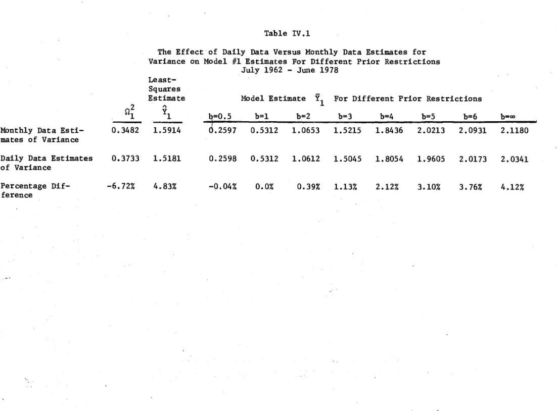
In Table IV.l, estimates for Model 111 are reported for the two different variance estimates and for different values of the upperbound restriction on Y
l under the assumption that Yl is constant over this sixteen-year period. As might be expected, for a "tight" prior (i.e., b small) and Y
YI(YI
~ b!2), the data have little weight in the posterior estimateY
I
•
For this reason, with b small, the differences in Y
I for the two different variance estimators are quite small. As b is increased, the data have greater weight in the estimate of Y
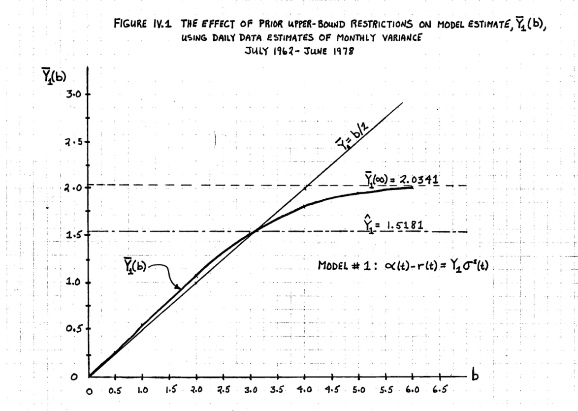
I and the effect on YI of the different variance estimators also increases. Figure IV.l plots
--- ~-.__..~..__..
Yl as a function of b using the daily data estimates of the monthly variances. As shown there,
the differences between Y
l for b as small as six and Yl for the diffuse prior (b
=
00) are rather small. Since no information is available which might provide a meaningful upperbound on aggregate relative risk aversion, the effects.of a finite b are analyzed no further and the diffuse prior assumption (b=
00) is made for the balance of the paper. That is, only the nonnegativity prior restriction is imposed upon the Y., j = 1,2,3.J
From Table IV.l, the effect of the two different variance estimators on the estimates of Model #1 is moderate with a percentage difference in .. the unrestricted regression estimate Y
l of about five percent and a percentage difference in the posterior estimate Y
l of about four percent. Both model parameter estimates were larger for the monthly-data variance estimates. However, as reported in Table IV.2, the
effect on the estimates of MOdels #2 and #3 is in the opposite direction and of considerably larger magnitude. As with Model #1, the percentage differences in the posterior estimates are somewhat smaller than the per-centage differences in the unrestricted regression estimates for both Models #2 and #3. However, for all estimates in these latter two models,
the percentage differences are in excess of 30 percent. The effect of the two variance estimators on the posterior density functions for each of
Table IV.1
The Effect of Daily Data Versus Monthly Data Estimates for Variance on Model #1 Estimates For Different Prior Restrictions
July 1962 - June 1978
MOnthly Data Esti-mates of Variance Daily Data Estimates of Variance Percentage Dif-ference Least-Squares Estimate 012 Y1")
"-0.3482 1.5914 0.3733 1.5181 -6.72% 4.83%Model Estimate Y1 For Different Prior Restrictions
~=0.5 b=l b=2 b=3 b=4 b=5 b=6 b=oo ,
.2597 0.5312 1.0653 1.5215 1.8436 2.0213 2.0931 2.1180 0.2598 0.5312 1.0612 1.5045 1.8054 1.9605 2.0173 2.0341 -0.04% 0.0% 0.39% 1.13% 2.12% 3.10% 3.76% 4.12%
, , ,
FIGURE
IV.~
TIfE
EFFECT
of PRIOR
IA.rreR-60lUJD
RE:>TRICT'OtJS
OM MODEL
E5TIH~T£1 ~(b)J
us,,.,c;
I>AIL'i
DATA f~T'HAT'SOF
MONTHL'(VARIAtJCE'
.JUL~ l~fD~-
'J'C.UJE
let7B
~(b)
3·0
. I -- r " .j . - i---; , ,MODEl.
*
1:
«l-t)-
rlt):::
Y~
(f'Ct)
i,- "
Y[oo)
="1.
0:5i1'
, '
, - - - - 1 - · - as -, -: ~ -:-_..._-..~. .---_.., ...._._.._.. _. ,
)
--
-
---1\ _ _ _ ' _ . _ _ --..-;._ ---fJ"-- ~ ~_-l1_=--1€lB1....
_~_ r I I I I I • • • I • I I I 'b
ji.!
o.s
o
=l.S
_._.: 1 ',1.0'
I :,
I~'O' .,. ,'o
O.S
1.0
1.5',
-1.D
:l.S,
3.0
3.5"
... 0
1·!,
5.0
"S.S,
'.0
'.5,
Table IV.2
The Effect of Daily Data Versus MOnthly Data Estimates of Variance on Different Models Estimates
with Nonnegative Restriction Only July 1962 - June 1978
MOnthly Data Estimates of Variance Daily Data Estimates of Variance Percentage Difference 0.3482 0.3733 -6.72% 1.5914 1.5181 4.83% 2.1180 2.0341 4.12% Model #2: ~(t) - r(t)
=
Y2cr (t)MOnthly Data Estimates of Variance Daily Data Estimates of Variance Percentage Difference 192 0.1123 0.1214 192 0.1806 0.1818 0% -37.82% -33.22% Model #3: ~(t) - r(t)
=
Y 3Monthly Data Estimates of Variance Daily Data Estimates of Variance Percentage Difference 172185 221708 -22.34% 0.0052 0.0053 0.0082 0.0083 -36.59% -35.37%
1:
Lt)-
'1
1
a& ")
.
. JULY
",% -
3"IJNi '97'
NOIINEGAT.vE PRIoR.,
Re$TRICTloN
ONLY
(b=oo)
.... DAILY
&~TU1ATEOF
MONTHLY
VARI"~C{ I•
I,
•
•
I•
I ...
-I : • i"
..
' ,Vi.
'=I.S'111---. •
•
•
-.
•
,
R R••
•
•
,
•
l-I I I,a
:
.
. I'.
,,,,,Y
_.
i
:
2.01411
I'.
,
••
•
1---I-+-.--ti----I---t....---+--==:::;.-::=--....
'11-1·0
S.O
'.0
7·0
0·0
·'0
.0
•, _ : -•_ _~• • _ . _~A'" +_ , ....:..._." ..-.- ;...MOm'HL
Y EST'MATE
OF
MOIJTHI..Y
VARIANt!
NON tlEGATIV£ PRIOR.
.RESTR.ac:.TlcN
ON"
Y
.<..
b=oo)
I ,. IYj.
=
l.seUi
~
I .,
J--:-·,
, I . · I · I . I . · I·' · I . I · I I .~Yi.:
%.1110
I I l I . I I I I . I · I. o,&...o-.--...
o--+-~t.HO--3-4.-0--41
....
-0-·
--s+.
0--=:::'+='"0::::::=='-'-+7.
/1
·0
i .._ - ,--~.-. _ ,., -.. .~.-..".-.. '--""".,-, _. ..F.GIlRI
IV. '5
PO'TER,olt
PROSABILITY
DiSTRIBUTION
FOR
Va.
MODIL
#
2. :
o((i)-t-tt)
=
Va.
O""lt)
Jw.y
11t-1-
"JUliE
'f7'
DA'LY £5T'
MATE
... OF HOttlTHL Y V/fRIANCE
.
NOtJNE~"T'v£PRIoR.
R&STR'C.T'OAI
ONLY(b-
00)
.
0-100·$0
1~o A , _V....
O.U2!.~
'.I
Y
I.=O.llI1
I , I I . .... . I I I I
MONTH..Y
eSTIMATE
OF NoN'httY v"'lAtleS
NOH
NI4ItT,V£
PRIoR.
RISTRIC.lION
ONLY... .c"=
00)
. j;
0-02S0
__ _DAII.'t
e,r'"ATE
_ _____. __ OF
"0"'11
a.
y",,,,.AIICE
___..
NOtI
NIGAT.VI
PRIoR.
.. __ . R&STIUt.T,olJ OHI.Y
_
.(b
:.0)
_•... __ ._._,_ .... _._. __ . .~,.. _. _ _ ._... _.._~.-.. •._._. ro' __ ' •.~ _ . _ - _. - • • • • •".
,
O· 0100 0.0'500-0:&00
MoO'1.
#
S:
ot(t)-rLt):=
'is
___
_
. __ _ .
3"IlLY ., '1-
:r...".
'1"
I I I I I I . I I A IYr·oot~Ys=·OO8.t
o
-ooSo
-0·0
'00-0
,so-o
-
~oo-o_. ... ...No,UIEGATIVE
PRioR
_ RiSTRIC.TION
ONLY
_.. _....
(b=
00)
"'''TNI.
'1
£ST'HAT£OF Mo-,THLY VAR,lUIcG
O· 010..0
0-01
SO O-OZOOo-ooso
AYS=.OOS%"'tVYS:
.00SI
-0·0
- ISO'O
-26-the three models are illustrated in Figures IV.2, IV.3, and IV.4. While these brief comparisons ,cannot be considered an analysis of the effects of measurement error in the variance estimates, they do serve as a warning against attaching great significance to the point estimates of the models.
From Table IV.2, it appears that for this period, the prior nonnega-tivity restriction is important only for Model #1 where for the same variance estimate, the percentage difference between Y
l and Yl is approximately 25 percent. The differences between the posterior
estimate and the unrestricted regression estimate for Model #2 and Model #3 are negligible. This result is further illustrated by inspection of the shapes and domains of the posterior density functions as
plotted in Figures IV.2, IV.3, and IV.4.
To further investigate the importance of the prior nonnegativity restriction, the differences between the pnoterior and unrestricted regression estimates are examined for fifty-tvlO years of data from
,--July 1926 to June 1978. These estimates are presented in Table IV.3 for both T=
52 years and T=
26 years. As inspection of this table immediately reveals, the percentage differences between Y. and Y.J J
are negligible for all three models with T
=
52, and for Models #2 and #3 with T=
26. For Model #1 with T=
26, the differences are small with an average about half of that found in the previous analysis from 1962-1978. As before, the posterior density functions for each of the models with T = 52 are plotted in Figures IV.5, IV.6, and IV.7.By the assumption that the Y. ,
Different Model Estimates for 52~Year and 26-Year Time Intervals July 1926 - June 1978
52-Year Intervals 26-Year Intervals 7/26-6/78 7/26-6/52 7/52-6/78 Average //1 : a.(t) - r(t) 2 Model =Y 1CJ (t)
ni
2.16246 1.6617 0.5007 1.0812 " Y 1 1.8932 1.5112 3.1608 2.3360 Y 1 1.8988 1.5588 3.2076 2.3832 Percentage Difference -0.30% -3.05% -1.46% -2.26% Model /12: a.(t) - r(t) = Y 2CJ(t)0.1
624 312 312 312 2"
Y 2 .1867 .2012 .1723 .1867 ,/ .1869 Y 2 .1867 .2012 .1725 Percentage Difference 0.0% 0.0% -0.16% -0.08% Model /13 : a.(t) - r(t) = Y 3rl
423624 144884 278740 211812 3 " Y 3 .0082 .0109 .0068 .0089-
.0082 .0109 .0068 .0089 Y 3 Percentage Difference 0.0% 0.0% 0.0% 0.0%... FIGIA.RE Iv.r
POSTERIOfl
PROBABILITY
DlsTRlauT'o~Fort
Ys.
"ODIiL
#'
~:
at
(i)-
r(t).
y~
(fIt'll
... .;rI&LY
1121. -
;JUliE.17'
... . .. --.. ..
•
.. ....•t.o
.
NOH IIIGAT'VE
PRIOR.
..
"STRIC.T'ON
ONLY
..._.._...( b.
CO)
Ys.
"·0
s·o
1-0
3·0
I I I I•
I I•
I I I•
I /..
. I .. II> . I\:I.I'1t,-~1'11.1"r
I0'0
···10
.... ..
·0
~__ ... -"._ ._ ._ ....__ •.. __ ._ .. __ ... _L.".MOl)£ L
#
2:
Q(t~)-
=
cr(.)
.. __ __
. _
~ItLY 111f. -
~UHEJ'
7 ,
NoN
NEGAT.VE
PR/ott
RISTRIC.TION
OIlL
Y
(b=
(0)
t I I I A , _'1t:""~I.,...YI.:
.llc."7
·S'·O
...-_IIIIt:;..~...__
~ ~ - . _...__
~...-__..._
YI.
. 0·0
0 · '0
0 ·
ao
0 · SO
tJ •
410
0 · 50
0 ·
'0
.. "-_..-_
..•...•.'.~..:._,-...--.. '._.._.- ' ,-,...---.--..---.._.._-- ..-._."._. _. ".FI6UR£
IV.1
PoSrlRloR.
PRolABIUTY DISTR'.WT,oN
FoR. Y
s
'NODaL
#
I:
ottt)-
rlt):
Y.
_._. _.
...
.
.
JULy ",,,-
3'Ur4E
Ict."
- -t.o·o
. __ NON
Ntt;AT,vEPI,O..
_.__ RISTR.C.T,ON Or4t
Y
_. __
(bcoo)
0·0100o·oaso
0'0,50
0·0100.
-l=.ootl
y~.ooal I .....,s
o·
00500·0
- .100·0
.-
0-0
---"'--'--'- -'-- ._.. -_.~.---.. _._..--~...•.. -.--~-- - - . - . - -~.__ .- ".•--- .- •.. -.-._ ~.." .'.f"-- .-. - -•• -'" -. , '." .. -.' I • _ ...•...•.._ •. _.__ , ...•...~ _~_. ._._~_. _ . __ ."._. ._0_ .•~_.,., 1.long time period, the number of observations N is quite large (624 for T
=
52 and 312 forasymptotic convergence of
T == 26). ,.. Y. +Y.
J J
Given the previously-demonstrated for large N, these findings were not entirely unexpected. However, if shorter time intervals over which Y
j is assumed to be constant are chosen, then the differences between Y. and Y. are not negligible.
J J
In Table IV.4, the different model estimates are presented for T
=
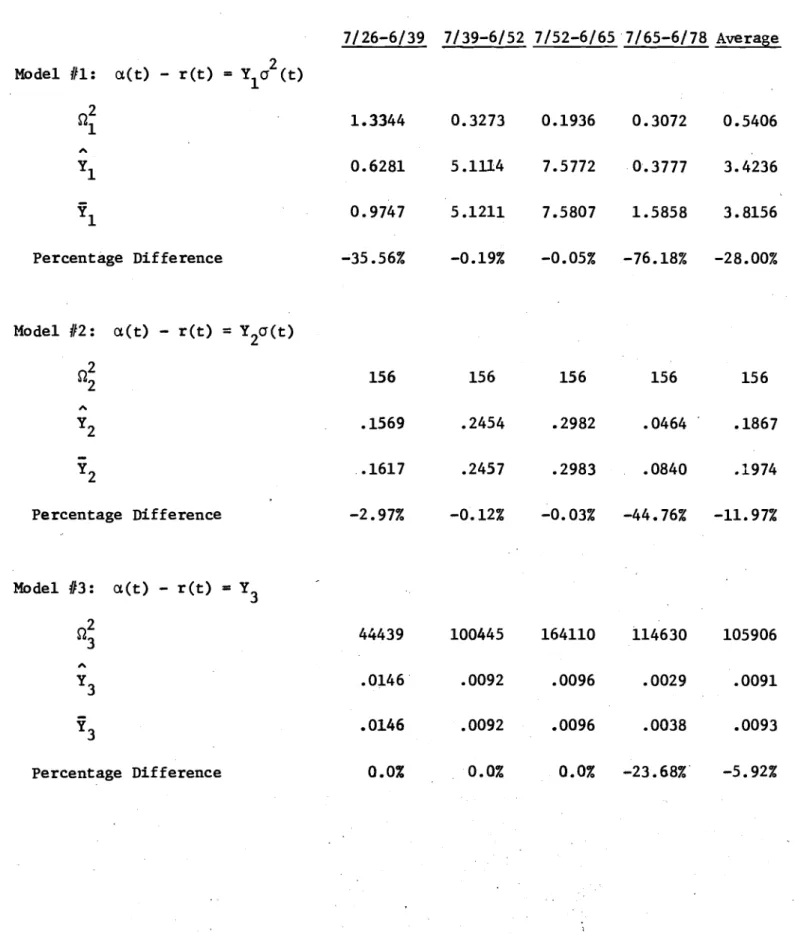
13 years (with N=
156). The average percentage difference between Y. and Y. for the four l3-year time periods ranged fromJ J
a high of 28 percent for Model /11 to a low of 6 percent for Model f!3
with Model #2 in the middle at a 12 percent difference. However, the percentage differences for each of the time periods are more important
' j :
than the average since by hypothesis, the using 13 years of data.
Y.
J can only be estimated In the 1965-1978 {ieriod, the percentage differences between the posterior estimate and the unrestricted regression estimate are
substantial for all three models. This was a period with a number of large negative realized excess returns on the market, and this is
precisely the tYpe of period in which the prior nonnegativity restriction can be expected to be important. The periods 1939-1952 and 1952-1965 did not have these large negative realized excess returns and corres-pondingly, the nonnegativity restriction was (expost) unimportant. The period 1926-1939 appears to be different from the other three in that the effect of the nonnegativity restriction is quite larg~ for Model /11; small for Model //2; and negligible for Model //3. However,
Table IV.4
Different MOdel Estimates for 13-Year Time Intervals July 1926 - June 1978 7/26-6/39 7/39-6/52 7/52-6/657/65-6/78 Average Model 111: a(t) - r(t) =Y 2 10" (t) 0.2 1.3344 0.3273 0.1936 0.3072 0.5406 1 " Y 1 0.6281 5.1114 7.5772 0.3777 3.4236 Y1 0.9747 5.1211 7.5807 1.5858 3.8156 Percentage Difference -35.56% -0.19% -0.05% -76.18% -28.00% Model /12: a(t) - r(t) = Y 20"(t) 0.22 156 156 156 156 156 " Y 2 .1569 .2454 .2982 .0464 .1867
-Y2 .• 1617 .2457 .2983 .0840 .1974 Percentage Difference -2.97% -0.12% -0.03% -44.76% -11. 97% Model 113: a(t) - r(t) = Y 3 0.2 44439 100445 164110 114630 105906 3 " Y 3 .0146· .0092 .0096 .0029 .0091 Y 3 .0146 .0092 .0096 .0038 .0093 Percentage Difference 0.0% 0.0% 0.0% -23.68%· -5.92%the results from this period are consistent with the others. This was a period of both large positive and negative realized excess returns with both large changes in variance and large variances especially in
the early 1930's when the market had a large negative average excess "
return. From the regression estimators, (II.Z), Y
l has in its numerator the unweighted average of the (logarithmic) realized excess returns. Y
Z has in its numerator the weighted average of these excess returns where the weights are such that each excess return is "deflated" by that month's estimate of the standard deviation. That is,
"
unlike Y
l in which each observed excess return has the same weight, Y
Z puts more weight on observed excess returns which occur in lower-than-average-standard-deviation months and less weight on those that occur on higher-than-average-standard-deviation months. Inspection of the regression estimator for Hodel 113 will show that the weighting of the realized excess returns is similar to that of Y
Z except the effect is more pronounced because each month's return is divided . by that month's variance. Hence, in a period such as the early
1930's when, expost, large negative excess returns occur in months
Y.
J
Of
and Y. will be largest in Model #1 and smallest in Model #3. J
course, just the opposite effect will occur in periods when, expost, where the variance is also quite large, the differences between
either large negative excess returns occur in months when the variance is small, or more likely, large positive excess returns occur in months when the variance is large and a number of negative excess returns occur in months when the variance is small.
In the 1966-1970
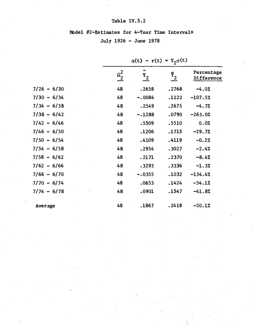
-29.-To provide further evidence in support of this explanation and to further underscore the importance of the nonnegativity constraint, especially as T becomes smaller, Tables IV.5.l, IV.5.2, and IV.5.3 provide the estimates for all three models for T
=
4 years (N=
48). In the 1930-1934 period, the regression estimates were negative for all three models with the largest percentage difference between Y. andJ Y
j occurring for Model #1 and the smallest for Model #3. In the 1938 -1942 period, the regression estimates for Model #2 and Model #3 were negative, and the ranking of the models by percentage differences between
and
Y
j was reversed from that of the 1930-1934 period.
period, the regression estimates for Model #1 and Model #2 are negative with the same model rankings as in the 1930-1934 period.
While the periods in which the regression estimates are negative demonstrate the necessity for the nonnegativity restriction most dramatically, it is not necessary that the estimatesbe negative to
Y. J
have large percentage differences between Y. and J in point 3re the 1970-1974 and 1974-1978 periods.
Y..
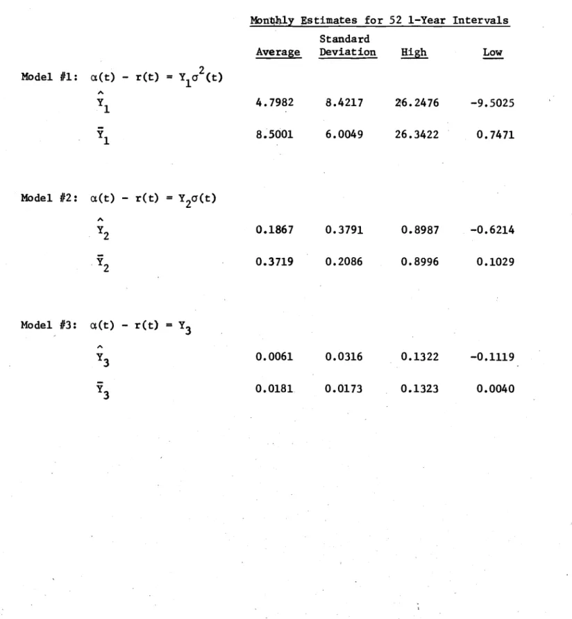
Two cases JAs expected, when T is further reduced from four years to one year, the effect of the nonnepati~ty.restrictionis even more. pronounced. The summary statistics for this case are presented in Table IV.6.
As a final illustration of the necessity for including the nonnegativity restriction, the estimates of Y
j and Yj (j
=
1,2,3) using the monthly...data variance estimator for the period 1962-1978 are compared with the corresponding estimates for the period 1965-1978.MOdel H1-Estimates for 4-Year Time Intervals July 1926 - June 1978 (l,(t) - r(t)
=
Y 2 1cr (t)r"z
,., Percentage Y 1 Y1 1 Difference 7/26 - 6/30 .1785 2.4778 3.1184 -20.5% 7/30 - 6/34 .8365 -0.1097 0.8337 -113.2% 7/34 - 6/38 .2276· 1.9389 2.6017 -25.5% 7/38 - 6/42 .2226 0.2156 1.7721 -87.8% 7/42 - 6/46 .0860 12.6511 12.6525 0.0% 7/46 - 6/50 •0787 1.9159 . 3.6625 -47.7% 7/50 - 6/54 .0553 12.2185 12.2459 -0.2% 7/54- 6/58 .0685 . 7.6509 7.8610 -2.7% 7/58 - 6/62 .0607 4.3146 5.3906 ""'20.0% 7/62 - 6/66 .0507 9.0518 9.2786 -2.4% 7/66 - 6/70 .0863 -2.2060 2.0534 -207.4% 7/70 - 6/74 .0909 0.9986 3.0443 -67.2% 7/74- 6/78 .1204 1.6183 2.9964 -46.0% Average .1664 4.0566 5.1932 -49.3%Table IV.5.2
MOdel H2-Estimates for 4-Year Time Intervals July 1926 - June 1978
aCt) - ret) =Y2a(t)
02 A Percentage Y2 Y2' 2 Difference 7/26 - 6/30 48 .2658 .2768 -4.0% 7/30 - 6/34 48 -.0084 .1122 -107.5% 7/34 - 6/38 48 .2549 .2675 -4.7% 7/38 - 6/42 48 -.1288 .0790 -263.0% 7/42 - 6/46 48 .5509 .5510 0.0% 7/46 - 6/50 48 .1206 .1715 -29.7% 7/50 - 6/54 48 .4109 .4119 -0.2% 7/54 - 6/58 48 .2954 .3027 -2.4% 7/58 - 6/62 48 . .2171 .2370 -8.4% 7/62 - 6/66 48 .3293 .3336 -1.3% 7/66 - 6/70 48 -.0355 .1032 -134.4% 7/70 - 6/74 48 .0653 .1424 -54.1% 7/74 - 6/78 48 .0901 .1547 -41.8% Average 48 .1867 .2418 -50.1%
MOdel #3~Estimates for 4-Year Time Intervals. July 1926 ~ June 1978 a(t) - r(t)
=
Y 3~i
x Percentage Y 1 Y3 3 Difference 7/26 - 6/30 22344 .0165 .0167 -1.2% 7/30 - 6/34 4091 -.0015 .0119 -112.6% 7/34 - 6/38 16124 .0183 .0185 -1.1% 7/38 - 6/42 19633 -.0149 .0026 -673.1% 7/42 - 6/46 29693 .0222 .0222 0.0% 7/46 - 6/50 33517 .0062 .0075 -17.3% 7/50 - 6/54 47626 .0126 .0126 0.0% 7/54 - 6/58 35062 .0111 .0113 -1.8% 7/58 - 6/62 43347 .0084 .0088 -4.5% 7/62 - 6/66 73342 .0088 .0089 -1.1% 7/66 - 6/70 30920 .0014 .0051 -72.5% 7/70 - 6/74 35864 .0031 .0056 -44.6% 7/74 - 6/78 32059 .0029 .0057 -49.1% Average 32586 .0073 .0106 -75.3%Table IV.6
Summary Statistics of Different MOdels Estimates for I-Year Time Intervals
July 1926 - June 1978
MOn~h1y Estimates for 52 I-Year Intervals
Standard
Average Deviation High Low
MOdel
111:
a.(t) - r(t)=
Y 2 1a (t),.
Y 1 4.7982 8.4217 26.2476 -9.5025 Y 1 8.5001 6.0049 26.3422 0.7471 MOdel #2: a.(t) - r(t)=
Y 2a(t) 0.1867 0.3719 0.3791 0.2086 0.8987 0.8996 -0.6214 0.1029 MOdel113:
a,(t) - r(t)=
Y 3,.
Y 3 0.0061 0.0316 0.1322 -0.1119 Y 3 0.0181 0.0173 0.1323 0.0040Since the variance estimates and return data axe identical for the l3-year overlapping period 1965-1978, the differences between the estimates
presented in Table IV.2 and those presented in Table IV.4 reflect the effect of a change from a l6-y.ear to a l3-year observation period. The three-year period 1962-1965 eliminated by this change was one in which the realized excess returns on the market were mostly positive .and the variances were relatively low.
For Model #1, the effect of this change on the posterior estimate Y
l is a 25.1 percent decline. While this was substantial, the effect on the regression estimate was much greater with a decline in y~
1 of 76.3 percent. The effect on the other model estimates is similar. For Model #2, the posterior estimate Y2 changes by 30.8 percent
A with a corresponding change in Y
2 of 58.7 percent. For Model #3, the change in Y
3 is 28.3 percent and the change in Y3 is 44.2 percent.
The substantial percentage change in both the Y
j and Y.J
. estimates from a relatively small change in the observation period illustrates the general difficulty in accurately estimating the parameters in an expected return model and underscores the importance of using as long a historical time series as is available. However, very long time series are not always available, and even when they are, it may not be reasonable to assume that the parameters to be estimated were stationary over that long a period. Therefore, given the relative stability of the Y. ·estimator by comparison with Y.,
J J
Having analyzed the empirical estimates of the
-31-in the specification of any such expected return model.
Y., we now examine J
the properties of the expected excess returns on the market implied by each of these models. For this purpose, it is ,!ssumed that the Y
j., (j
=
1,2,3), were constant over the entire period 1926-1978, and therefore, T equals 52 years. Of course, this assumption iscertainly open to question. However, given the much-discussed problems with the variance estimators and the exploratory spirit with which this paper is presented, further refinements as to the best estimate of T are not warranted here. Moreover, as discussed in Section II,
the current state-of-the-art model implicitly makes this assumption by using as its estimate of the expected excess return on the market, the sample average of realized excess returns over the longest data period available.
Using the estimated Y. and the time series of estimates for the J
market variances, monthly time series of the expected excess return on - the market were generated for each of the three models over the 624
months from July 1926 to June 1978. As shown in Figures IV.5, IV.6, and IV.7, with T equal to 52 years, the posterior density functions for all three models are virtually symmetric and the differences between and Y.
J are negligible. Hence, for
Y. J T
=
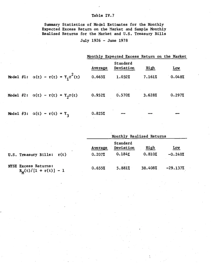
52 years, the monthly time series of expected excess returns using the unrestricted regression estimates would be identical to those presented here.The. summary statistics for thesemon~hlytime series are reported in Table IV.7 and they include the sample average, standard deviation
and the highest and lowest values. Of course, the expected excess
r~turn estimate for Model 113 is simply a constant. In Table IV.7, the same summary statistics are presented for the realized excess returns on the market and for the realized returns on the riskless asset.
Inspection of Table IV.7 shows that the average of the expected excess returns varies considerably across the three models. The
"Constant-Preferences" Model III is the lowest wUhan average of 0.665 percent per month or, expressed as an annualized excess return, 8.28 percent per year. The "Cons tant-Price-'o f-Risk" Model 112 is the
highest with an annualized excess return average of 12.04 percent per year. The "Constant-Expected-Excess-Return" Model 1/3 is almost exactly midway between the other two models with an annualized average of
10.36%. The sample average of the realized excess returns on the market was 0.655 per.:'-ent per month, or, annualized, 8.15 percent per year • . This sample average is also the point estimate for the expected excess . return on the market according to the state-of-the-art model.
Even with these large differences in the average estimates, it is unlikely that any of these models could be rejected by the realized return data. The variance of the unanticipated part of the returns on the market is much larger than the variance of the change in expected return. That is, the realized returns are a very "noisy" series for detecting differences among models of expected return.
In examining the average excess returns in Table IV.7, one might be tempted to conclude that Model III "looks" a little better because its
Table IV.7
Summary Statistics of Model Estimates for the Monthly Expected Excess Return on the Market and Sample Monthly Realized Returns for the Market and U.S. Treasury Bills
July 1926 - June 1978
Monthly Expected Excess Return on the Market Standard
Average Deviation
1!!.8!!.
Low Model /11: aCt) - ret)=
Y1C1 (t)2 0.665% 1.032% 7.161% 0.048%Model #2: aCt) - ret)
=
Y 2C1(t)Model #3: aCt) - ret)
=
Y 30.952%
0.825%
0.570% 3.628% 0.297%
Monthly Realized Returns Standard
Average Deviation High Low U.S. Treasury Bills: ret) 0.207% 0.184% 0.810% -0.240%
NYSE Excess Returns:
0.655% 5.881% 38.408% -29.137% l\r(t)/[1
+
ret)] - 1average is so close to the sample average6f realized excess returns. However, as inspection of (11.2.1) makes clear, the regression estimator Y
l is such that this must always be the case when the variance estimator is of the type used here. This observation brings up an important issue with respect to estimates based upon the state-of-the-art model.
If the strict formulation of that model is that the expected excess return on the market is a constant or at least, stationary over time, then the least-squares estimate of that constant is given by Y
3 in MOdel #3. However, from Table IV.7,the annualized difference between Y
3 and the sample realized return average is 221 basis points. This difference is quite large when considered in the context of
portfolio selection and corporate finance applications. The reason for the difference is that the sample average of realized returns is only a least-squares estimate if the variance of returns over the
period is con.::~t.ant • If the variance is no t cons tan t, and it isn't, then the estimator should be adjusted for heteroscadasticity in the .. "error" terms. This is exactly what the estimator Y
3 does. Of course, the sample average of realized returns is a consistent
estimator and the measurement error problem in the variance estimates rule out formal statistical comparison. However, the large difference reported here should provide a warning against neglecting the effects of changing variance in such estimations and simply relying upon
"consistency" even when the observation period is as long as 52 years. As mentioned, the sample average of the realized returns will provide an efficient estimate of the average expected excess return if
-34-Model 111 is the correct specification. However, even if that is the belief, then for capital market and corporate finance applications, Yl times the current variance will provide a better estimate of the current expected excess return than the state-of-the-art model because it takes into account the current level of risk associated with the market.
A similar argument applies to using the ratio of the sample
average of the realized excess returns to the sample standard deviation for estimating the Price of Risk under the hypothesis that it is
constant, or at least, stationary over time. From Table IV.7, using the realized return statistics, the estimate of the Price of Risk is 0.114 per month whereas the least-squares estimate Y
2 which takes into account the changing variance rates is 0.1867 per month. Again, this difference is quite large.
To further underscore the importance of taking into account the change in the variance rate when estimating the expected return on the market, we close this section with a brief examination of the time series of market variance estimates. The average monthly variance rates for the market returns are presented in Table IV.8 for the thirteen successive four-year periods from July 1926 to June 1978. Over the entire 52-year period, the average annual standard deviation of the market return was 20.4 percent. However, as is clearly demonstrated in Table IV.8, the variance rate can change by'a substantial amount from one four-year period to another, and it is significantly different from this average in many of the four-year periods.
Successive Four-Year Average Monthly Variance Estimates for The Return on the Market
July 1926 - June 1978 Dates 7/26 - 6/30 7/30 - 6/34 7/34 - 6/38 7/38 - 6/42 7/42 - 6/46 7/46 - 6/50 7/50 - 6/54 7/54 - 6/58 7/58 - 6/62 7/62 - 6/66 7/66 - 6/70 7/70 - 6/74 7/74 - 6/78. Average
Average Monthly Variance*
a
2(t) .003719 .017427 .004742 .004638 .001792 .001640 .001152 .001427 .001265 .001056 .001798 .001894 .002508 .003467 Percentage Change From Previous Period368.59% -72.79% -2.19% -61.36% -8.48% -29.76% 23.87% -11.35% -16.52% 70.27% 5.34% 32.42%
-35-It has frequently been reported that the market was considerably more volatile in the pre-World War II period than it has been in the post-war period. That observation is confirmed here with an average annual standard deviation of 27.9 percent for the period July 1926 to June 1946 versus 13.8 percent for the period July 1946 to June 1978. However, a significant part of this difference is explained by the extraordinarily large variance rates in the 1930-1934 period. Thus, if this period is excluded, then the average annual standard deviation for the other twelve four-year periods is 16.6 percent.
Because the state-of-the-art model assumes a constant variance
rate, the large differences in variance rates among the various subperiods causes this model's estimates to be quite sensitive to the time period of history used. So, for example, if the 1930-1934 is excluded, then
th~ estimated Market Price of Risk based upon the other forty-eight years of data changes by 33 percent for the state-of-the-art model
estimator. However, this same exclusion caases Model #2's estimate, Y2' . to change by only 8 percent.