On the Approximate Maximum Likelihood Estimation for Diffusion Processes

Munich Personal RePEc Archive

On the Approximate Maximum

Likelihood Estimation for Diffusion

Processes

Chang, Jinyuan and Chen, Songxi

2011

Online at

https://mpra.ub.uni-muenchen.de/46279/

On the Approximate Maximum Likelihood Estimation

for Diffusion Processes

Jinyuan Chang

_{and Song Xi Chen}

1 _{Department of Business Statistics and Econometrics}

Guanghua School of Management and Center for Statistical Science Peking University

2 _{Department of Statistics}

Iowa State University

Emails: [email protected]; [email protected]

Abstract

The transition density of a diffusion process does not admit an explicit expression in general, which prevents the full maximum likelihood estimation (MLE) based on discretely observed sample paths. A¨ıt-Sahalia (1999, 2002) proposed asymptotic expansions to the transition densities of diffusion processes, which lead to an approximate maximum likelihood estimation (AMLE) for parameters. Built on A¨ıt-Sahalia (2002, 2008)’s analysis on the AMLE, we establish the consistency and convergence rate of the AMLE, which reveal the roles played by the number of terms used in the asymptotic density expansions and the sampling interval between successive observations. We find conditions under which the AMLE has the same asymptotic distribution as that of the full MLE. A first order approximation to the Fisher information matrix is proposed.

AMS 2000 subject classifications: Primary 62M05; Secondary 62F12.

Keywords and phrases:Asymptotic expansion; Asymptotic normality; Consistency; Dis-crete time observation; Maximum likelihood estimation.

1

Introduction

survey on the financial applications of continuous-time stochastic models which were largely the diffusion processes. Fan (2005) provided an overview on nonparametric estimation for diffusion processes. Other related works include Bibby and Sørensen (1995), Wang (2002), Fan and Zhang (2003), Fan and Wang (2007), Mykland and Zhang (2009) and A¨ıt-Sahalia, Mykland and Zhang (2011).

Estimating parameters of diffusion processes faces several challenges. One is that despite being continuous-time models, the processes are only observed at discrete time points rather than observed continuously over time. The discrete observations prevent the use of the relatively straight forward likelihood expressions (Prakasa Rao, 1999) available for continuously observed diffusion processes. Another challenge is that despite the diffusion processes are Markovian, their transition densities from one time point to the next do not have finite analytic expressions except for only a few specific processes. This means that the efficient maximum likelihood estimation (MLE) can not be readily implemented for most of these processes.

In path breaking works, A¨ıt-Sahalia (1999, 2002) established series expansions to approximate the transition densities of univariate diffusion processes. Similar expansions have been proposed for multivariate processes in A¨ıt-Sahalia (2008). These density approximations, as advocated by A¨ıt-Sahalia, are then employed to form approximate likelihood functions, which are maximized to obtain the approximate maximum likelihood estimators (AMLEs). A¨ıt-Sahalia (2002, 2008) demonstrated that the approximate likelihood converges to the true likelihood as the number of terms in the series expansions goes to infinity. He also provided some results on the consistency of the AMLEs. Numerical evaluations of the transition density approximations as conducted in A¨ıt-Sahalia (1999), Stramer and Yan (2007a, 2007b) and others have shown good performance in the numerical approximation of the underlying transition densities. The approach has opened a very accessible route for obtaining parameter estimators for diffusion processes, and for esti-mating other quantities which are functions of the transition density, as commonly encountered in finance. Indeed, A¨ıt-Sahalia and Kimmel (2005, 2010) demonstrated two such applications in stochastic volatility models and the affine term structure models, respectively. Tang and Chen (2009) provided some results on the AMLE based on the one-term expansion for the mean-reverting processes. They revealed that there was an extra leading order bias term in the AMLE due to the density approximation.

Although the above mentioned results on the transition density approximation and the AMLE had been provided, there are some key questions remain to be addressed. One is on the consis-tency of the AMLE. While A¨ıt-Sahalia (2002, 2008) contained some results on consisconsis-tency, there is more to be explored. There are two key ingredients in A¨ıt-Sahalia’s density approximation. One is J, the number of terms used in the approximation, and the other isδ, the length of the sampling interval between successive observations. In this paper, we study explicitly the roles

played by J and δ on the consistency of the AMLE, and quantify their roles on the convergence

rate. Another question is under what conditions onJ andδ, the AMLE has the same asymptotic

distribution as the full MLE. Here, we consider two regimes: (i) δ is fixed and J _{→ ∞}; (ii) J is

fixed but δ _→ 0, representing two views of asymptotics. In the case of δ _→ 0, it is found that

J >2 is necessary to ensure the AMLE having the same asymptotic normality as the MLE. Like

The paper is organized as follows. In Section 2, we outline the transition density approxima-tions of A¨ıt-Sahalia (1999, 2002). Some preliminary analysis needed for studying the AMLE is presented in Section 3. Section 4 establishes the consistency and convergence rates of the AMLE. Asymptotic normality of the AMLE and its equivalence to the full MLE are addressed in Section 5. Section 6 discusses the approximation for the Fisher information matrix. Simulation results are reported in Section 7. Technical conditions and details of proofs are relegated to Appendix.

2

Transition Density Approximation

Consider a univariate diffusion process (Xt)t≥0 defined by a stochastic differential equation

dXt=µ(Xt;θ)dt+σ(Xt;θ)dBt, (2.1)

where µ and σ are respectively the drift and diffusion functions, Bt is the standard Brownian

motion. Both the drift and diffusion functions are known except for an unknown parameter vectorθ taking values in a set Θ_⊆Rd.

Given a sampling interval δ > 0, let fX(x|x0, δ;θ) be the transition density of Xt+δ given

Xt =x0 for (x0, x)∈ X × X, where X is the domain of Xt. Despite the parametric forms of the

drift and the diffusion functions are available in (2.1), a closed-form expression forfX(x|x0, δ;θ)

is not generally available for most of the processes. In most cases, the density is only known to satisfy the Kolmogorov backward and forward partial differential equations. In path-breaking works, A¨ıt-Sahalia (1999, 2002) proposed asymptotic expansions to approximate the transition density.

The approach of A¨ıt-Sahalia is the following. He first transformed Xt to a diffusion process with unit diffusion function by

Yt=γ(Xt;θ) :=

Z Xt _du

σ(u;θ), (2.2)

which satisfies dYt=µY(Yt;θ)dt+dBt, where

µY(y;θ) =

µ(γ−1_(y;θ);θ)

σ(γ−1_(y;θ);θ) −

1 2

∂σ ∂x(γ

−1_(y;θ);θ).

Let fY(y|y0, δ;θ) be the transition density of Yt+δ given Yt =y0. The two density functions are

related according to

fX(xt|xt−1, δ;θ) = σ−1(xt;θ)·fY(γ(xt;θ)|γ(xt−1;θ), δ;θ). (2.3)

To ensure convergence of the expansions, A¨ıt-Sahalia standardizedYt+δbyZt+δ =δ−1/2(Yt+δ−

y0). Let fZ(z|y0, δ;θ) denote the conditional density ofZt+δ given Zt= 0, which is related to fY by

fZ(z_|y0, δ;θ) =δ1/2fY(δ1/2z+y0|y0, δ;θ).

Let_{Hj(z)_}∞

j=1 be the Hermite polynomials

Hj(z) = φ−1(z)

dj_φ(z)

which are orthogonal with respect to the standard normal densityφ, namelyR Hj(z)Hk(z)φ(x)dx= 0 if j ₆=k. A formal Hermite orthogonal series expansion to the density fZ(z_|y0, δ;θ) is

f_ZH(z_|y0, δ;θ) =φ(z)

∞

X

j=0

ηj(y0, δ;θ)Hj(z) (2.4)

where the coefficients

ηj(y0, δ;θ) = (j!)−1 Z

Hj(z)fZ(z|y0, δ;θ)dz

= (j!)−1

E[Hj(δ−1/2(Yt+δ−y0))|Yt =y0;θ].

The last conditional expectation has no analytic expression in general, although it may be simu-lated using the method proposed in Beskos et al. (2006). A¨ıt-Sahalia proposed Taylor expansions for this conditional expectation with respect to the sampling intervalδ based on the infinitesimal generator of Yt. For twice continuously differentiable function g, the infinitesimal generator of

Yt is

Aθg(y) =µY(y;θ)

∂g ∂y +

1 2

∂2_g

∂y2. (2.5)

A K-term Taylor series expansion to _E[Hj(δ−1/2(Yt+δ−y0))|Yt=y0;θ] is

E[Hj(δ−1/2(Yt+δ−y0))|Yt=y0;θ]

= K

X

k=0

AkθHj(δ−1/2(y−y0))|y=y0 δk

k!

+E[_Ak_θ+1Hj(δ−1/2(Yt+δ∗−y₀))|Y_t=y₀;θ]

δk+1

(k+ 1)!.

(2.6)

Substituting (2.6) to the orthogonal expansion (2.4) followed by gathering terms according to the powers of δ, aJ-term expansion to the transition density fY(y, δ|y0;θ) is

f_Y(J)(y_|y0, δ;θ) = δ−1/2φ

y₋y0

δ1/2

exp

Z y

y0

µY(u;θ)du

_XJ

j=0

cj(y|y0;θ)

δj

j!,

where c0(y|y0;θ)≡1 and for j >1,

cj(y|y0;θ) =j(y−y0)−j Z y

y0

(w₋y0)j−1

·

λY(w;θ)cj−1(w|y0;θ) +

1 2

∂2_c

j−1(w|y0;θ)

∂w2

dw.

HereλY(y;θ) =−{µ2Y(y;θ) +∂µY(y;θ)/∂y}/2.

Transforming back from y tox via (2.2) and (2.3), the J-term expansion tofX(x|x0, δ;θ) is

f_X(J)(x_|x0, δ;θ) = σ−1(x;θ)δ−1/2φ

γ(x;θ)₋γ(x0;θ)

δ1/2

·exp

Z x

x0

µY(γ(u;θ);θ)

σ(u;θ) du

_XJ

j=0

cj(γ(x;θ)|γ(x0;θ);θ)

δj

Although it employs the Hermite polynomials and has the Gaussian density as the leading term as an Edgeworth expansion does, the transition density expansion is not an Edgeworth expansion. This is because the latter is for density functions of statistics admitting the central limit theorem, which differs from the current context of expanding the transition density. A¨ıt-Sahalia (2002)

demonstrated that as J _{→ ∞},

f_X(J)(x_|x0, δ;θ)→fX(x|x0, δ;θ) (2.7)

uniformly with respect to θ _∈ Θ and x0 over compact subsets of X. The convergence is also

uniformly with respect tox over subsets of _X depending on the property ofσ(x;θ). Define

A1(x|x0, δ;θ) =−log{σ(x;θ)} −

1

2δ{γ(x;θ)−γ(x0;θ)}

2

,

A2(x|x0, δ;θ) = Z x

x0

µY(γ(u;θ);θ)

σ(u;θ) du and

A3(x|x0, δ;θ) = log _XJ

j=0

cj(γ(x;θ)|γ(x0;θ);θ)δj/j!

.

IfP∞_j=0|cj(y|y0, δ;θ)|δj/j!<∞onY × Y with probability one, whereY is the domain ofYt, we

can define Ae3(x|x0, δ;θ) = log{P∞j=0cj(y|y0;θ)δj/j!}. Then, the result in (2.7) implies that

logfX(x|x0, δ;θ)

=₋log√2πδ+A1(x|x0, δ;θ) +A2(x|x0, δ;θ) +Ae3(x|x0, δ;θ).

(2.8)

Expression (2.8) is the starting point for our analysis.

Given a set of discrete observations _{Xtδ}nt=1 with equal sampling length δ of the diffusion

process (Xt)t≥0, to simplify notations, we writeXt for Xtδ, and hideδ in the expressions for the transition densityfX and its approximations. At the same time, we usef andf(J) to expressfX and f_X(J) respectively. Based on the J-term expansion to the true transition density, the J-term approximate log-likelihood function given in A¨ıt-Sahalia (2002) is

ℓ(_n,δJ)(θ) = ₋nlog√2πδ+ n

X

t=1

A1(Xt|Xt−1, δ;θ)

+ n

X

t=1

A2(Xt|Xt−1, δ;θ) +

n

X

t=1

A3(Xt|Xt−1, δ;θ).

Let ˆθ(_n,δJ) = arg maxθ∈Θℓ(n,δJ)(θ) be the approximate MLE (AMLE) and ˆθn,δ be the true MLE that maximizes the full likelihood

ℓn,δ(θ) = n

X

t=1

logf(Xt|Xt−1, δ;θ).

3

Preliminaries

Under regular circumstances as assumed by Condition (A.2) (ii) in Appendix, the full MLE ˆθn

and the J-term approximate MLE ˆθ(nJ) satisfy their respective likelihood score equations so that

n

X

t=1

∇θlogf(Xt|Xt−1, δ; ˆθn) =

n

X

t=1

∇θlogf(J)(Xt|Xt−1, δ; ˆθn(J)) = 0. (3.1)

SubtractingPn_t=1∇θlogf(J)(Xt|Xt−1, δ;θ0) from both sides of (3.1),

n

X

t=1

∇θlogf(J)(Xt|Xt−1, δ; ˆθ(nJ))− n

X

t=1

∇θlogf(J)(Xt|Xt−1, δ;θ0)

= n

X

t=1

∇θ[Ae3(Xt|Xt−1, δ;θ0)−A3(Xt|Xt−1, δ;θ0)]

+ n

X

t=1

∇θlogf(Xt|Xt−1, δ; ˆθn)−

n

X

t=1

∇θlogf(Xt|Xt−1;θ0).

(3.2)

Carrying out Taylor expansions on both sides of (3.2), we can get

1

n

n

X

t=1

∇2θθlogf(J)(Xt|Xt−1, δ;θ0)·(ˆθn(J)−θ0)

+ 1

2[Ed⊗(ˆθ

(J)

n −θ0)′]·

1

n

n

X

t=1

∇3θθθlogf(J)(Xt|Xt−1, δ; ˜θ)·(ˆθ(nJ)−θ0)

= 1

n

n

X

t=1

∇θ[Ae3(Xt|Xt−1, δ;θ0)−A3(Xt|Xt−1, δ;θ0)]

+ 1

n

n

X

t=1

∇2θθlogf(Xt|Xt−1, δ;θ0)·(ˆθn−θ0)

+ 1

2[Ed⊗(ˆθn−θ0)

′_]

· _n1

n

X

t=1

∇3θθθlogf(Xt|Xt−1, δ; ¯θ)·(ˆθn−θ0)

(3.3)

where Ed is thed×d identity matrix, ˜θ is on the joint line between ˆθn(J) and θ0, and ¯θ is on the

joint line between ˆθn and θ0. Here we define

∇3θθθlogf(Xt|Xt−1, δ;θ) :=   

∂3_logf(X

t|Xt−1, δ;θ)/∂θ∂θ′∂θ1

...

∂3_logf(X

t|Xt−1, δ;θ)/∂θ∂θ′∂θd

which is ad2 _{×d matrix, and ∇}3

θθθlogf(J)(Xt|Xt−1, δ;θ) is similarly defined. Furthermore, let

Fn(θ0, J, δ) = n−1

n

X

t=1

∇2θθ[Ae3(Xt|Xt−1, δ;θ0)−A3(Xt|Xt−1, δ;θ0)],

Un(θ0, J, δ) = n−1

n

X

t=1

∇θ[Ae3(Xt|Xt−1, δ;θ0)−A3(Xt|Xt−1, δ;θ0)] and

Nn(θ0, J, δ) = n−1

n

X

t=1

∇2θθlogf(J)(Xt|Xt−1, δ;θ0).

Then, (3.3) can be written as

Nn(θ0, J, δ)(ˆθ(nJ)−θ0) + ∆n1(ˆθ(nJ), θ0)

=Un(θ0, J, δ) + [Nn(θ0, J, δ) +Fn(θ0, J, δ)] (ˆθn−θ0) + ∆n2(ˆθn, θ0)

(3.4)

where ∆n1(ˆθ(nJ), θ0) and ∆n2(ˆθn, θ0) denote the remainder terms whose explicit expressions can

be obtained by matching (3.3) with (3.4).

The expansion (3.4) is the starting point in our studies for the consistency and asymptotic distribution of the AMLE. Indeed, the asymptotic properties of the AMLE will be evaluated under two regimes regardingJ and δ. The first one is that

δ is fixed but J _{→ ∞}, (3.5)

which is the situation considered in A¨ıt-Sahalia (2002). The second regime allows that

J is fixed, δ_→0 but nδ _{→ ∞}, (3.6)

which is more tuned with an implementation of the density approximation with a fixed number of terms.

We will first present some results which are valid for any fixed J and δ. Let _||A_||2 =

{ρ(A′_A)}1/2 _{be the spectral norm of a matrix A, where ρ(A}′_{A) denotes the largest eigen-value}

of A′_{A. The following proposition describes properties for the quantities appeared in (3.4).}

Proposition 1 Under Conditions (A.1), (A.3)-(A.4), (A.6)-(A.7) given in Appendix, there ex-ists a positive constant ∆ such that for any positive integer J and δ _∈(0,∆),

(a) E{Fn(θ0, J, δ)}, E{Un(θ0, J, δ)} and E{Nn(θ0, J, δ)} exist;

(b) ∆n1(ˆθn(J), θ0) =Op{||θˆ(nJ)−θ0||2}2 and ∆n2(ˆθn, θ0) =Op{||θˆn−θ0||22} as n→ ∞.

LetI(δ) =₋E∇2

θθlogf(Xt|Xt−1, δ;θ0) be the Fisher information matrix, which we assume is

invertible in Condition (A.5). It is expected that the expected value of Nn(θ0, J, δ), denoted by

N(θ0, J, δ), will converge to −I(δ), asJ → ∞ for each fixed δ orJ being fixed but δ→ 0. The

following proposition bounds the difference between N(θ0, J, δ) and −I(δ) for each fixed J and

δ.

Proposition 2 Under Conditions (A.1), (A.4), (A.6)-(A.7) given in Appendix, there exist two positive constants∆¯ andC, that are not dependent onJ andδ, such that for any positive integer

J and δ_∈(0,∆)¯ ,

As I(δ) is invertible for each fixed δ > 0, Nn(θ0, J, δ) will be invertible with probability

approaching one as J _{→ ∞} for a fixed δ. However, if δ_→0, the limit of the Fisher information

I(0) := limδ→0I(δ), as well as N(θ0, J,0), may be singular. This is the case for some

Ornstein-Uhlenbeck processes as shown in Section 6. The following proposition provides another account onN(θ0, J, δ) and its deviation from−I(δ), as well as the convergence of N−1(θ0, J, δ)U(θ0, J, δ),

where U(θ0, J, δ) denotes the expected value of Un(θ0, J, δ) for each pair of fixed J and δ.

Proposition 3 Under Conditions (A.1), (A.3)-(A.7) given in Appendix, there exist two con-stants C1, C2, that are not dependent on J and δ, and a constant ∆ > 0 such that for any

positive integer J and δ_∈(0,∆),

||N−1(θ0, J, δ)I(δ) +Ed||2 6C1δJ and ||N−1(θ0, J, δ)U(θ0, J, δ)||2 6C2δJ.

The next proposition describes the convergence rate for the difference between the first deriva-tives of the full log-likelihood and the approximate log-likelihood.

Proposition 4 Under Conditions (A.1), (A.4), (A.6)-(A.7) given in Appendix, there exist two finite positive constants ∆e and C, not dependent onJ and δ, such that for any J, δ _∈(0,∆]e and

n,

E

sup θ∈Θ

n−1_{· ∇}θ[ℓn,δ(θ)₋ℓ_n,δ(J)(θ)]

2

6CδJ+1.

The following proposition together with Proposition 4 is needed to establish the consistency of the AMLE.

Proposition 5 Under Conditions (A.1), (A.3)-(A.4), (A.6)-(A.7) given in Appendix, there ex-ists a constant ∆˙ >0 such that

sup θ∈Θ

1

n

n

X

t=1

∇θlogf(Xt|Xt−1, δ;θ)−E∇θlogf(Xt|Xt−1, δ;θ) 2

p

− →0

for (i) δ_∈(0,∆]˙ being fixed, n_{→ ∞}, or (ii) n_{→ ∞}, δ_→0 but nδ _{→ ∞}.

As the full MLE ˆθn is a key bridge for the AMLE, we report in the following proposition the

asymptotic normality of the MLE which covers both cases of fixed δ and diminishing δ case.

Proposition 6 Under Conditions (A.1)-(A.7) given in Appendix,

√

nI1/2_(δ)(ˆθ

n−θ0)

d

−

→N(0, Ed) as nδ3 → ∞,

where Ed is d×d identity matrix.

The requirement of nδ3 _{→ ∞ in the above proposition is to cover the case where I(0) =}

limδ→0I(δ) is singular, as spelt out in the proof given in the appendix. If such case is ruled

4

Consistency

We consider in this section the consistency of the AMLE ˆθ(nJ) and establish its convergence rate under the two asymptotic regimes given in (3.5) and (3.6) respectively. The two asymptotic regimes were also considered in A¨ıt-Sahalia (2002, 2008). For a fixed sampling interval δ, A¨ıt-Sahalia (2002) proved that there existed a sequence Jn → ∞such that ˆθn(Jn)−θˆn

p

→0 under Pθ0

asn _{→ ∞}, wherePθ0 is the underlying probability measure. Based on the consistency of ˆθn, we

know that the consistency of ˆθn(Jn) is hold. For a fixed J, A¨ıt-Sahalia (2008) proved that there existed a sequence_{δn}vanishing to zero such that √nI1/2(δn)(ˆθn,δn(J) −θ0) =Op(1).

In this paper, we will give more explicit guidelines on how to select the afore-mentioned

sequences Jn and δn so that the AMLE is consistent. Our study here begins with (3.1), which

together with Propositions 4 and 5 lead to the following result on the consistency of the AMLE under the two asymptotic regimes, respectively.

Theorem 1 Under Conditions (A.1)-(A.4), (A.6)-(A.7) given in Appendix, θˆn(J)−θ0

p

−

→0under either (i) δ _∈(0,∆e _∧∆]˙ being fixed, J _{→ ∞} and n _{→ ∞}, or (ii) J being fixed, n _{→ ∞}, δ _→0

but nδ _{→ ∞}.

By Proposition 2 and Condition (A.5), multiplyN−1_(θ

0, J, δ) on both sides of (3.4), we have

ˆ

θ(_nJ)₋θ0

= N−1Un+N−1(Nn+Fn)(ˆθn−θ0)−N−1(Nn−N)(ˆθ(nJ)−θ0) −N−1∆n1(ˆθn(J), θ0) +N−1∆n2(ˆθn, θ0).

(4.1)

From this together with Proposition 4 and Theorem 1, we can establish the convergence rate of the AMLE.

Theorem 2 Under Conditions (A.1)-(A.7) given in Appendix,

ˆ

θ(_nJ)₋θ0 =

Op{δJ+1+ (nδ)−1/2}, if δ ∈(0,∆e ∧∆]˙ is fixed and J → ∞;

Op{δJ+ (nδ)−1/2}, if J is fixed, δ →0 but nδ3 → ∞.

The above theorem reveals the impacts of the sampling interval δ and the number of terms

J used in the density approximation on the convergence rate. In particular, the rate of AMLE

has an extra δJ+1 _{or δ}J _{term in addition to the standard rate (nδ)}−1/2 _{of the full MLE. This}

extra term is the result of the density approximation. And its particular form suggests that the sampling interval δ has to be less than 1 in order to make the AMLE ˆθ(nJ) converge to θ0. It is

apparent that the higher the J is, the less impact the extra term has on the AMLE ˆθn(J).

5

Asymptotic Distribution

In this section, we consider the asymptotic distribution of the AMLE ˆθn(J). Our investigations

are organized according to two asymptotic regimes: (i) δ fixed, J _{→ ∞} and (ii) J fixed, δ _→0

5.1

Fixed

δ

,

J

_{→ ∞}

This is a simple case to treat. Under this setting, we note from Proposition 2 and Condition (A.5) that, N−1_(θ

0, J, δ) = O(1) uniformly for any J. Utilizing the result in Theorem 2, the

expansion (4.1) becomes

ˆ

θ_n(J)₋θ0 =N−1Un+ (ˆθn−θ0) +Op(n−1/2δJ−1/2+n−1δ−1+δ2J+2).

Hence, note that Un=Op(δJ+1),

√

nI1/2(δ)(ˆθ_n(J)₋θ0)

= √nI1/2(δ)(ˆθn−θ0) +Op(δJ−1/2+n−1/2δ−1+n1/2δJ+1).

Ifnδ2J+2 _{→0, then}

√

nI1/2(δ)(ˆθ(_nJ)₋θ0)

d

−

→N(0, Ed).

Therefore, the AMLE has the same asymptotic distribution as the full MLE ˆθn. This is attained by requestingnδ2J+2 _{→0 in addition toJ → ∞. Ifnδ}2J+2 _{→c >0, the AMLE is still asymptotic}

normal but would have an inflated variance due to the contribution from the first term involving

Un. Apart from this, the asymptotic mean will no longer be zero. Hence, it is much desirable to have nδ2J+2 _{→ 0. The latter condition prescribes a rule on the selection of the J =J}

n(δ). By choosing anǫ >0 so that δ2J+2 _=n−1−ǫ _{for each pair of n and δ, then}

J =Jn(δ) = −1−ǫ

2 logδ logn−1>

−1

2 logδlogn−1.

The integer truncation of the above lower bound plus one can be used as a reference value for the number of term used in the density approximation for each given pair of (n, δ).

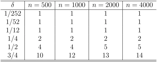
Table 1 reports such reference values of J assigned by the above formula for a set of (n, δ) combinations commonly encountered in empirical studies. It shows that for monthly frequency

or less (δ 6 1/12), one term approximation is adequate, and for δ = 1/4, J = 2 is needed.

However, there is a dramatic increase inJ as the sampling length is larger than 1/4: demanding at least four terms for δ = 1/2 (half yearly) or at least ten terms for δ = 3/4. The number of terms also increases for these higher δ values as n increases, although the rate of this increase

is much slower than that as δ is increased. The latter may be understood that for a given δ,

as n increases, the chance of having extreme values in the tails of the transition distribution

increases. As the density approximation is less accurate in the tails than in the main body of the distribution, there is a need for having more terms in the density approximation.

5.2

J

fixed,

δ

_→

0

but

nδ

_{→ ∞}

Our starting point is the expansion (4.1). As Nn −N = Op{(nδ)−1/2}, N−1(Nn−N) = op(1)

if nδ3 _{→ ∞, which is also required in the asymptotic normality of the full MLE as outlined in}

Proposition 6. We will show in the following that nδ3 _{→ ∞ is also necessary to ensure AMLE}

sharing the same asymptotic distribution as the full MLE. It is understood that in order for ˆθn(J) having the same asymptotic distribution as ˆθn, it is required that

N−1_{Un, N}−1_∆n

Table 1: The least approximation term selection to guarantee the AMLE has the same asymp-totic distribution as the full MLE for special sampling intervalδ and sample size n

δ n= 500 n = 1000 n = 2000 n= 4000

1/252 1 1 1 1

1/52 1 1 1 1

1/12 1 1 1 1

1/4 2 2 2 2

1/2 4 4 5 5

3/4 10 12 13 14

We will demonstrate in the following that the above requirements can be attained bynδ3 _{→ ∞}

and J > 2. Hence, under these circumstances, ˆθn(J) has the same asymptotic distribution as ˆθn. Later we will demonstrate that this equivalence in the asymptotic distribution is quite unlikely for J = 1. Our analysis needs to expand (3.2) to the quadratic terms. To this end, let us define

Mn(θ0, J, δ) = n−1

n

X

t=1

∇3θθθlogf(J)(Xt|Xt−1, δ;θ0) and

Tn(θ0, J, δ) =n−1

n

X

t=1 ∇3

θθθlogf(Xt|Xt−1, δ;θ0).

By further expanding to quadratic terms, (4.1) can be written as

ˆ

θ(_nJ)₋θ0

= N−1Un+N−1(Nn+Fn)(ˆθn−θ0)−N−1(Nn−N)(ˆθ(nJ)−θ0) − 1

2N

−1_[E

d⊗(ˆθ(nJ)−θ0)′]Mn(ˆθn(J)−θ0)

+1₂N−1_[E

d⊗(ˆθn−θ0)′]Tn(ˆθn−θ0) −N−1∆n˜ 1(ˆθn(J), θ0) +N−1∆n˜ 2(ˆθn, θ0),

(5.2)

where ˜∆n1(ˆθ(nJ), θ0) and ˜∆n2(ˆθn, θ0) are remainder terms. Using the same method in the proof

of Proposition 1, it can be shown that ˜∆n1(ˆθn(J), θ0) = Op{||θˆn(J) − θ0||32} and ˜∆n2(ˆθn, θ0) =

Op{||θˆn−θ0||32}.

In order to make ˆθ(nJ) have the same asymptotic distribution as ˆθn, the two quadratic terms on the right of (5.2) have to be smaller order of ˆθn(J)−θ0 and ˆθn−θ0 respectively, namely

N−1[Ed⊗(ˆθn(J)−θ0)′]Mn(ˆθn(J)−θ0) = op{||θˆn(J)−θ0||2}

or equivalently

N−1_[E

d⊗(ˆθn(J)−θ0)′] =op(1); (5.3)

and

or equivalently

nδ3 _{→ ∞}, (5.4)

since ˆθn−θ0 =Op{(nδ)−1/2} and N−1 =O(δ−1).

As ˆθn(J)−θ0 =Op{δJ+ (nδ)−1/2}, (5.3) requires that δJ−1+n−1/2δ−3/2 →0. Hence, in order to make ˆθn(J) have the same asymptotic distribution as ˆθn, it is necessary to have

J >2 and nδ3 _{→ ∞. (5.5)}

Now we consider the case of J = 1. To ensure the remainder terms N−1_∆n

1(ˆθn(J), θ0) and

N−1_∆n

2(ˆθn, θ0) are negligible, by a similar argument applied above for the case of J > 2, it is

also necessary to assume nδ3 _{→ ∞. From Theorem 2, ˆθ}(1)

n −θ0 = Op{δ+ (nδ)−1/2}. To gain insight on the situation, we need to find out the order of magnitude of the quadratic term in (5.2), namely the order of magnitude of

Sn=N−1[Ed⊗(ˆθn(1)−θ0)′]Mn(ˆθ(1)n −θ0)−N−1[Ed⊗(ˆθn−θ0)′]Tn(ˆθn−θ0).

With this notation, (5.2) can be written as

ˆ

θ(_nJ)₋θ0 =N−1Un+N−1(Nn+Fn)(ˆθn−θ0)− 1₂Sn +op{(nδ)−1/2}+Op(δ2).

(5.6)

Define an operator between two vectors A and B:

A_∗B = [Ed⊗A′]MnB + [Ed⊗B′]MnA.

By repeated substitutions, it can be shown that

Sn= 1₂N−1[(N−1Un)∗(N−1Un)] + 1₂N−1

₁ 2Sn

∗ 12Sn

−N−1(N−1Un)_∗ 1₂Sn

+op(δ).

As Un = Op(δ2) for J = 1 and N−1 = O(δ−1), it can be deduced from the above equation thatSn =Op(δ). Hence, forJ = 1 if we requirenδ3 → ∞, the quadratic termSn will contribute to the leading order of ˆθ(1)n −θ0. If we do not requirenδ3 → ∞, then the sum of remainder terms,

N−1_∆n˜

1(ˆθn(J), θ0) +N−1∆n˜ 2(ˆθn, θ0) will not be controlled. Hence, if J = 1, it is very likely that

the asymptotic distribution of ˆθn(J) will differ from that of ˆθn unlessUn= 0 with probability one. In the rare case ofUn = 0, it is possible for ˆθn(1) and ˆθn to share the same limiting distribution.

Therefore, in order to guarantee that ˆθn(J) has the same asymptotic distribution as ˆθn under

δ _→ 0, we need to use the AMLE based on at least two-term expansions, while satisfying

nδ3 _{→ ∞, which we will assume in the rest of this section.}

Note that ˆθ(nJ)−θ0 =Op{δJ + (nδ)−1/2}. Then, ˆ

θ_n(J)₋θ0 = N−1Un+ (ˆθn−θ0)

Furthermore,

√

nI1/2(δ)(ˆθ(_nJ)₋θ0)

=√nI−1/2(δ)I(δ)N−1Un+√nI1/2(δ)(ˆθn−θ0) +Op(δJ−3/2)

+√nI−1/2(δ)I(δ)N−1_·Op(δ2J +n−1δ−1)

=√nI1/2(δ)(ˆθn−θ0) +Op(δJ−3/2+n−1/2δ−3/2+n1/2δJ+1/2).

Hence, for any J >2 such that nδ3 _{→ ∞ and nδ}2J+1 _→0, √

nI1/2(δ)(ˆθ(_nJ)₋θ0)

d

−

→N(0, Ed).

This result shows that, when δ vanishes to zero, in order to guarantee the AMLE has the same

asymptotic distribution as full MLE, we need to pick the approximation order J > 2, while

maintaining nδ3 _{→ ∞ and nδ}2J+1 _→0.

The following theorem summarizes the asymptotic normality under both asymptotic regimes.

Theorem 3 Under Conditions (A.1)-(A.7) given in Appendix,

√

nI1/2(δ)(ˆθ(nJ)−θ0)

d

−

→N(0, Ed),

for (i) δ _∈ (0,∆e _∧∆]˙ being fixed, n _{→ ∞}, J _{→ ∞} but nδ2J+2 _{→ 0 or (ii) J > 2 being fixed,}

n_{→ ∞}, δ_→0 but nδ3 _{→ ∞ and nδ}2J+1 _→0.

5.3

Asymptotic bias and variance

The remainder of this section is devoted to the consideration of the asymptotic bias and variance of the AMLE under the two asymptotic regimes. Given our analysis in the early part of this section, our consideration will be focused on the situations where the asymptotic normality of

the AMLE can be assumed, namely under (i) δ being fixed,J _{→ ∞},n _{→ ∞} but nδ2J+2 _{→0 or}

(ii) J >2 being fixed, δ_→0,nδ3 _{→ ∞ but nδ}2J+1 _→0.

In the case of δ being fixed and J _{→ ∞}, from (5.2) and providednδ2J+2 _{→0, we have}

ˆ

θ_n(J)₋θ0 = N−1Un+N−1(Nn+Fn)(ˆθn−θ0)−N−1(Nn−N)N−1Un

−N−1(Nn−N)N−1(Nn+Fn)(ˆθn−θ0) − 12N

−1_{E

d⊗[N−1Un+N−1(Nn+Fn)(ˆθn−θ0)]′} ·Mn[N−1Un+N−1(Nn+Fn)(ˆθn−θ0)]

+ 1

2N

−1_[E

d⊗(ˆθn−θ0)′]Tn(ˆθn−θ0) +Op(n−3/2) = N−1Un+ [Ed−N−1(Nn−N)]N−1(Nn+Fn)(ˆθn−θ0)

+Op(n−1/2δJ+1) +Op(n−3/2).

Then, the leading order bias of ˆθn(J) is

B(θ0, J, δ)

=N−1U +En[Ed−N−1(Nn−N)]N−1(Nn+Fn)(ˆθn−θ0) o

and the leading order variance is

V(θ0, J, δ) = N−1I(δ)V ar(ˆθn)I(δ)N−1. (5.8)

In the case of J >2 being fixed,δ _→0 and nδ3 _{→ ∞ but nδ}2J+1 _{→0, it can be shown by a}

similar argument to that for the fixed δ case above, the asymptotic bias and variance have the

same forms as (5.7) and (5.8), respectively. Both (5.7) and (5.8) will be used to calibrate with the simulated bias and variance in the simulation study in Section 7. ForJ = 1 andδ_→0, there are difficulties in obtaining an expression for the bias of the AMLE in general due to the same dilemma in controlling the reminder terms and the quadratic termSn as outlined in Section 5.2.

6

Approximating Fisher Information Matrix

We demonstrate in this section that the approximation of the transition density provides a

way to approximate the Fisher information matrix. Fisher information matrix I(δ) is a key

quantity associated with inference based on the full MLE. It defines the asymptotic efficiency and convergence rate. From Proposition 2, a natural candidate to approximate I(δ) is ₋N(θ0, J, δ)

based on the J-term expansion. To simplify our expedition, our consideration here is focused

under the following diffusion process

dXt=µ(Xt;η)dt+σ(Xt;ξ)dBt, (6.1)

whereη= (η1,· · ·, ηd1)

′ _{and ξ= (ξ}

1,· · · , ξd2)

′ _{are distinct drift and diffusion parameters}

respec-tively. The whole parameter θ = (η′_{, ξ}′₎′_{. Here, we provide an explicit expression N(θ}

0,1, δ)

based on the one-term density expansion. Expressions for higherJ values may be made via more

extensive derivations.

Recall that the one-term (J = 1) transition density approximation is

logf(1)(x_|x0, δ;θ)

=₋ 1

2log 2πδ−logσ(x;ξ)− 1

2δ(γ(x;ξ)−γ(x0;ξ))

2

+

Z x

x0

µ(u;η)

σ2_(u;ξ)−

1 2σ(u;ξ)

∂σ(u;ξ)

∂u

du

+ log_{1 +c1(γ(x;ξ)|γ(x0;ξ);θ)·δ},

where

c1(γ(x;ξ)|γ(x0;ξ);θ) =

1 2

−

µ(x;η)

σ(x;ξ) −

µ(x0;η)

σ(x0;ξ)

+ 1

2

∂σ(x;ξ)

∂x −

∂σ(x0;ξ)

∂x0

− Z x

x0

µ(u;η)

σ(u;ξ) − 1 2

∂σ(u;ξ)

∂u

2

du σ(u;ξ)

Z x

x0 du σ(u;ξ).

Then,

∂2_logf(1)

∂ηi∂ηj =

Z x

x0

∂2_µ(u;η)

∂ηi∂ηj

du

σ2_(u;ξ) +δ·

∂2_c 1

∂ηi∂ηj 1 1 +c1δ −

δ2_· ∂c1 ∂ηi

∂c1

∂ηj 1 (1 +c1δ)2

,

∂2_logf(1)

∂ηi∂ξj

= ₋2

Z x

x0

∂µ(u;η)

∂ηi

∂σ(u;ξ)

∂ξj

du

σ3_(u;ξ) +δ·

∂2_c 1

∂ηi∂ξj 1 1 +c1δ −

δ2 _·∂c1 ∂ηi

∂c1

and

∂2_logf(1)

∂ξi∂ξj

=₋ ∂

2_σ(x;ξ)

∂ξi∂ξj 1

σ(x;ξ) +

∂σ(x;ξ)

∂ξi

∂σ(x;ξ)

∂ξj

1

σ2_(x;ξ)

− 1

δ

Z x

x0

∂σ(u;ξ)

∂ξi

du σ2_(u;ξ)

Z x

x0

∂σ(u;ξ)

∂ξj

du σ2_(u;ξ)

+1

δ

Z x

x0 du σ(u;ξ)

Z x

x0

∂2_σ(u;ξ)

∂ξi∂ξj 1

σ2_(u;ξ) −

∂σ(u;ξ)

∂ξi

∂σ(u;ξ)

∂ξj

2

σ3_(u;ξ)

du

+

Z x

x0

6µ(u;ξ)

σ4_(u;ξ) −

∂σ(u;ξ)

∂u

1

σ3_(u;ξ)

∂σ(u;ξ)

∂ξi

∂σ(u;ξ)

∂ξj

−

2µ(u;ξ)

σ3_(u;ξ) −

∂σ(u;ξ)

∂u

1 2σ2_(u;ξ)

∂2_σ(u;ξ)

∂ξi∂ξj

+

∂2_σ(u;ξ)

∂u∂ξi

∂σ(u;ξ)

∂ξj

+ ∂

2_σ(u;ξ)

∂u∂ξj

∂σ(u;ξ)

∂ξi

1 2σ2_(u;ξ)

− ∂

3_σ(u;ξ)

∂u∂ξi∂ξj 1 2σ(u;ξ)

du

+δ_· ∂

2_c 1

∂ξi∂ξj 1 1 +c1δ −

δ2_· ∂c1 ∂ξi

∂c1

∂ξj 1 (1 +c1δ)2

.

Letµi, µij and so on denote partial derivatives with respect toηi,ηi andηj, respectively; and

σi and σx,j and so on denote partial derivatives with respect to ξi, and x and ξj, respectively. Then, it can be shown that

∂2_c 1

∂ηi∂ηj

x=x0

=₋σ−2µiµj −µσ−2µij+σ−1µijσx− 1 2µxij,

∂2_c 1

∂ηi∂ξj

x=x0

= 2µσ−3µiσj −σ−2µiσxσj+σ−1µiσxj

∂2c1

∂ξi∂ξj

x=x0

=₋3µ2σ−4σiσj+ 2µσ−3σxσiσj+µ2σ−3σij −µσ−2σxσij

−µσ−2σxiσj−µσ−2σxjσi+µσ−1σxij+ 1

4σxxσij − 1 4σxiσxj

−1₄σxσxij+ 1

4σxxiσj + 1

4σxxjσi+ 1

4σσxxij.

Let_A denote the infinitesimal generator of the diffusion process (6.1), which is similar to (2.5). Define

g1(x, x0) = Z x

x0

σiσ−2du

Z x

x0

σjσ−2du

and

g2(x, x0) = Z x

x0

σ−1du

Z x

x0

σ−2σij −2σ−3σiσj

du.

Ag_1|x=x0 = (σ

−2_σ

iσj)|x=x0,

A2g1|x=x0 = (2µ

2_σ−4_σ

iσj −8µσ−3σxσiσj+ 4σ−2σx2σiσj + 2σ−2µxσiσj + 2µσ−2σxiσj + 2µσ−2σxjσi−2σ−1σxσxiσj−2σ−1σxσxjσi

−2σ−1σxxσiσj+ 1

2σxiσxj+ 1

2σxxiσj+ 1

2σxxjσi)|x=x0,

Ag_2|x=x0 = σ

−1_σ

ij −2σ−2σiσj,

A2g2|x=x0 = (−4µ

2_σ−4_σ

iσj + 20µσ−3σxσiσj + 2µ2σ−3σij −4σ−2µxσiσj

−15σ−2σ2_xσiσj−7µσ−2σxσij −6µσ−2σxiσj−6µσ−2σxjσi + 2σ−1µxσij + 6σ−1σxxσiσj+ 9σ−1σxσxiσj+ 9σ−1σxσxjσi + 3σ−1σ2_xσij + 3µσ−1σxij−2σxxσij−

5 2σxσxij

−4σxiσxj −2σxxiσj −2σxxjσi+σσxxij)|x=x0.

Hence, from the above expressions,

E

∂2_logf(1)

∂ηi∂ηj

=δ_·E

∂2_c 1

∂ηi∂ηj

+O(δ2) =: δ_·N11(1)+O(δ2),

E

∂2_logf(1)

∂ηi∂ξj

=δ_·E

∂2_c 1

∂ηi∂ξj

+O(δ2_{) =: δ·N}(1)

12 +O(δ2)

and

E

∂2_logf(1)

∂ξi∂ξj

=_−E{σ−1σij +σ−2σiσj} −E[Ag1|x=x0] +E[Ag2|x=x0]

− δ₂·E[_A2g1|x=x0] + δ

2 ·E[A

2_g

2|x=x0] +δ·E

∂2_c 1

∂ηi∂ηj

+O(δ2)

=:₋2E(σ−2σiσj) +δ·N22(1)+O(δ2),

where

N₁₁(1) =E

−σ−2µiµj −µσ−2µij+σ−1µijσx− 1 2µxij

,

N₁₂(1) =E 2µσ−3µiσj −σ−2µiσxσj+σ−1µiσxj

,

N₂₂(1) =E

−6µ2σ−4σiσj+ 16µσ−3σxσiσj + 2µ2σ−3σij−3σ−2µxσiσj − 19

2 σ

−2_σ2

xσiσj

− 9

2µσ

−2_σ

xσij −5µσ−2σxiσj −5µσ−2σxjσi+σ−1µxσij + 4σ−1σxxσiσj

+11

2 σ

−1_σ

xσxiσj + 11

2 σ

−1_σ

xσxjσi+ 3 2σ

−1_σ2

xσij + 5 2µσ

−1_σ

xij− 3 4σxxσij

− 5₂σxiσxj − 3

2σxσxij−σxxiσj −σxxjσi+ 3 4σσxxij

Thus,

N(θ0,1, δ) = δ·N (1)

11 δ·N (1) 12

δ_·N₁₂(1)T ₋2_·E(σ−2_σ

iσj) +δ·N22(1) !

+O(δ2). (6.2)

We learn from Proposition 2 that ₋N(θ0,1, δ) provides a leading order approximation to

I(δ) with a reminder term at the order of δ2_{. Equation (6.2) confirms that as δ → 0, given the}

asymptotic normality of the full MLE ˆθn as conveyed by Proposition 6, that the convergence rate of the full MLE for the drift parametersη is (nδ)−1/2 _{whereas that for the diffusion parameters}

ξ is n−1/2_{, faster than the drift parameter estimator. Our study confirms the results of Gobet}

(2002), Sorensen (2007) and Tang and Chen (2009).

In the rest of the section, we will derive the Fisher information matrix approximation for two specific diffusion processes. Both are widely employed in modeling of the interest rate dynamics.

6.1

Vasicek’s Model

Consider Vasicek’s Model (Vaiscek, 1976),

dXt=κ(α−Xt)dt+σdBt, (6.3)

which is also the Ornstein-Uhlenbeck process. The conditional distribution ofXt given Xt−1 is

Xt|Xt−1 ∼N

Xt−1e−κδ+α(1−e−κδ),

1 2σ

2_κ−1₍₁

−e−2κδ)

and the stationary distribution of_{Xt} is

Xt ∼N

α,σ

2

2κ

. (6.4)

The log of the transition density is

logf(Xt|Xt−1, δ;θ)

=₋ 1

2logπ− 1

2log σ

2_κ−1₍₁

−e−2κδ)₋(Xt−Xt−1e

−κδ_−α(1−e−κδ₎₎2

σ2_κ−1_(1−e−2κδ₎ . Letθ = (κ, α, σ)T _{and P(X}

t, Xt−1, θ) =Xt−Xt−1e−κδ−α(1−e−κδ), then

P(Xt, Xt−1, θ)|Xt−1 ∼N

0,1

2σ

2_κ−1_(1−e−2κδ₎

. (6.5)

The second derivatives of logf(Xt|Xt−1, δ;θ) are, respectively,

∂2_logf

∂κ2 =−

1 2κ2 +

2δ2_e2κδ (e2κδ₋₁₎2 −

2κδ2_(X

t−1−α)2

σ2_(e2κδ₋₁₎

+ 4δe

2κδ_[(1−κδ)e2κδ_{−(1 +κδ)]P}2_(X

t, Xt−1, θ)

σ2_(e2κδ₋₁₎3

∂2_logf

∂α2 =−

2κ(eκδ₋₁₎2

σ2_(e2κδ₋₁₎,

∂2_logf

∂σ2 =

1

σ2 −

6κe2κδ_P2

σ4_(e2κδ ₋₁₎,

∂2_logf

∂κ∂α =

2κδ(Xt−1−α)(eκδ−1)

σ2_(e2κδ₋₁₎ +P(Xt, Xt−1, θ)L2(Xt−1, θ),

∂2_logf

∂κ∂σ =

2e2κδ_[e2κδ_{−(1 + 2κδ)]P}2

σ3_(e2κδ₋₁₎2 +P(Xt, Xt−1, θ)L3(Xt−1, θ)

and ∂

2_logf

∂α∂σ =P(Xt, Xt−1, θ)L4(Xt−1, θ),

where Li(Xt−1, θ), fori= 1,· · · ,4 are measurable functions of Xt−1 for given θ.

From (6.4) and (6.5), it yields that the information matrix of θ= (κ, α, σ)T _{is I(δ) = (I} ij)_3×3 where

I11=

1 2κ2 +

δ[κδ+κδe2κδ_−2e2κδ_{+ 2]}

κ(e2κδ₋₁₎2 =

δ

2κ +O(δ

2_{), I}

12 =I21= 0,

I13 =I31 =

(1 + 2κδ)₋e2κδ

σκ(e2κδ₋₁₎ =−

δ

σ +O(δ

2_{), I} 22=

2κ(eκδ₋₁₎2

σ2_(e2κδ ₋₁₎ =

κ2_δ

σ2 +O(δ 2_),

I23 =I32 = 0, and I33 =

2

σ2.

These mean that

I(δ) =



 δ·(2κ)

−1 ₀

−δ_·σ−1

0 δ_·κ2_σ−2 ₀

−δ_·σ−1 _{0 2σ}−2 

+O(δ2). (6.6)

Hence, I(0) = limδ→0I(δ) is singular, an issue we have raised earlier and led us to assume

δI−1_{(δ)’s largest eigen-value being bounded in Condition (A.5).}

Using the approximation formula in (6.2), we have

N(θ,1, δ) =

  −

δ_·(2κ)−1 _{0 δ·σ}−1

0 ₋δ_·κ2_σ−2 ₀

δ_·σ−1 _{0 −2σ}−2 

+O(δ2).

It means the leading order term of₋N(θ,1, δ) is identical with that of the true Fisher information matrix in (6.6).

6.2

Cox-Ingersoll-Ross Model

Consider Cox-Ingersoll-Ross (CIR) Model (Cox, Ingersoll and Ross, 1985)

dXt=κ(α−Xt)dt+σ

p

XtdBt. (6.7)

which is also Feller (1952)’s square root processes.

Let θ= (κ, α, σ)T _{and c= 4κσ}−2_(1−e−κδ₎−1_{, the conditional distribution of cX}

t given Xt−1

is

where the distribution is a non-central χ2 _{distribution with degree of freedom ν = 4κασ}−2 _and

non-central parameter λ=cXt−1e−κδ. The transition density ofXt+δ given Xt is

f(Xt|Xt−1, δ;θ) =

c

2e

−u−vv

u

q/2

Iq(2√uv),

where u =cXt−1e−κδ/2, v =cXt/2, q = 2κα/σ2−1 >0 and Iq is the modified Bessel function of the first kind of order q. If 2κα > σ2_{, then the stationary distribution of {X}

t} is

Xt∼Γ

2κα σ2 ,

σ2

2κ

. (6.8)

The log transition density function is

logf(Xt|Xt−1, δ;θ) = logc−(u+v) +

q

2(logv−logu) + logIq(2

√

uv)₋log 2.

Although the second partial derivations of the log transition density function can be derived after some labor that involved with differentiating the modified Bessel function of first kind, acquiring an expression for the Fisher information matrix is a rather hard task, largely due to the difficulty in deriving the expectations. In contrast, using the approximation formula (6.2), we can obtain the approximation for opposite Fisher information matrix

N(θ0,1, δ) = 

 NN1121 NN1222 NN1323

N31 N32 N33 

+O(δ2),

where

N11 =δ·σ−2·E{Xt−1(α−Xt)2}, N12 =N21 =δ·E

2κσ−2X_t−1(α₋Xt)₋ 1

2X

−1

t

,

N13=N31=−δ·2κσ−3·E{Xt−1(α−Xt)2}, N22 =δ·κ2σ−2·EXt−1,

N23 =N32=−δ·2κ2σ−3·E{Xt−1(α−Xt)} and

N33= 2σ−2−δ·3κσ−2+δ·E

6κ2σ−4X_t−1(α₋Xt)2₋6κσ−2X_t−1(α₋Xt) + 9

4X

−1

t +σ−1Xt−1

.

More explicit form of the approximation may be obtained by cultivating the marginal distribution of Xt. Under (6.8), we can get

EX_t−1 = σ

2

2κα₋σ2 and EXt =α.

Then,

N11 =δ·

α2_σ2 _−2κα2_+ασ2

2κασ2 _−σ4 , N12=N21=δ·

4κασ2_−σ4_−8κ2_{α+ 4κσ}2

4κασ2_−2σ4 ,

N13 =N31=−δ·

2κα2_σ2_−4κ2_α2_{+ 2κασ}2

2κασ3_−σ5 , N22=δ·

κ2

2κα₋σ2,

N23 =−δ·

2κ2_ασ2_−4κ3_{α+ 2κ}2_σ2

2κασ3_−σ5 , and

N33 =

2

σ2 +δ·

24κ2_α2_σ2 _−48κ3_α2_{+ 48κ}2_ασ2_−24κασ4_{+ 36κσ}4_{+ 4σ}5_{+ 9σ}6

8κασ4_−4σ6 .

Using₋N(θ0,1, δ), we can get the approximation of Fisher information matrix. This

6.3

Observed Fisher Information

The major application for the asymptotic normality of both the full and approximate MLEs is for statistical inference ofθ, which include confidence regions and testing hypotheses for θ. For such purposes, the Fisher informationI(δ) needs to be estimated. A natural candidate would be

−Nn(ˆθn(J), J, δ). Although it converges toI(δ) at the rate of Op{(nδ)−1/2+δJ}orOp{(nδ)−1/2+

δJ+1_{} depending on δ is fixed or diminishing, −Nn(ˆθ}(J)

n , J, δ) may not be nonnegative definite, which can hinder the acquisition of _{−Nn(ˆθn(J), J, δ)}1/2. To get around this issue, by noticing that I(δ) is the variance of the likelihood score, we consider

e

In(θ, J, δ) = 1

n

n

X

t=1

[_∇θlogf(J)(Xt|Xt−1, δ;θ)][∇θlogf(J)(Xt|Xt−1, δ;θ)]′

as an estimator of I(δ). The following theorem shows that by replacing I(δ) with Ien(ˆθ(nJ), J, δ) in Theorem 3.

Theorem 4 Under Conditions (A.1)-(A.7) given in Appendix,

√

nIe_n1/2(ˆθ_n(J), J, δ)(ˆθ(_nJ)₋θ0)

d

−

→N(0, Ed),

for (i) δ _∈ (0,∆e _∧∆]˙ being fixed, n _{→ ∞}, J _{→ ∞} but nδ2J+2 _{→ 0 or (ii) J > 2 being fixed,}

n_{→ ∞}, δ_→0 but nδ3 _{→ ∞ and nδ}2J+1 _→0.

Confidence regions and testing hypothesis can be readily carried out by utlizing the above results.

7

Simulation

We report results from simulation studies which are designed to confirm the theoretical findings on the AMLE as reported in the earlier sections. To allow verification with the full MLE, we considered the Vasicek and CIR diffusion models reported in the previous section as both

models permit the full MLE. The two asymptotic regimes were experimented: the fixed δ and

the diminishing δ with nδ3 _{→ ∞.}

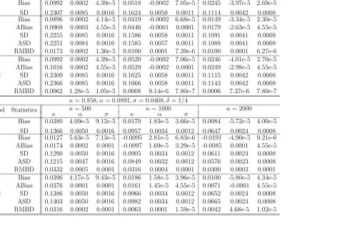
The first part of the simulation is about the case which δ is fixed. The parameters used

in the simulated Vasicek and CIR models were θ = (κ, α, σ)′ _{= (0.858,0.0891,0.0468)}′ _and

θ = (κ, α, σ)′ _{= (0.892,0.09,0.1817)}′_{, respectively. The sampling interval δ was 1/12 and 1/4,}

and the order of the density approximation J was 1 and 2, respectively. For each δ and J,

the sample size n was set at 500, 1000 and 2000 respectively. In addition to bias and standard

deviation, we consider

RMSD(n, J, δ) =

q

E||θˆ(nJ)−θˆn||22,

the square root of the expected square of modulated deviations between ˆθ(nJ) and ˆθn, as an overall performance measure.

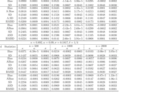
Table 2 and 3 summarize the simulation for the fixed δ case. They report the average bias

and standard deviation (SD) for the full MLE and AMLEs with J = 1 and J = 2, as well as the

give the simulation results more perspectives and to confirm the derived approximate bias and variance formulae in Section 5, we also computed the asymptotic bias and standard deviation

based on the formulae (5.7) and (5.8). We observe from Tables 2 and 3 that at each δ (1/12

and 1/4) experimented, the bias and the standard deviation of all the estimators for the three

parameters became smaller as n increased. These confirmed the consistency of the estimators.

The tables also showed that there was a good agreement among the three estimators in terms of

the performance measures. It appeared that the bias and the variance of the AMLE withJ = 1

andJ = 2 were quite comparable to each other. However, by comparing RMSD, it was clear that

in most of the cases (except for n = 500 of CIR model), the RMSD for J = 2 was smaller than

J = 1, signaling the AMLE with J = 2 was closer to the full MLE than that of the AMLE with

J = 1. This indicates that the AMLEs with J = 2 were indeed closer to those with J = 1, as

confirmed by our early analysis. The asymptotic bias and standard deviation predicted for the

AMLE withJ = 1 and 2 offer more insights, and showed good agreement between the simulated

results and the predicted values by the theory, which is very assuring. We also observe that for

δ= 1/4, the AMLE withJ = 2 performs better than AMLE withJ = 1, which somehow reflects

Table 1 which shows that J = 2 is preferred than J = 1 at this frequency. When δ was fixed at

1/12, we see the performance between J = 1 andJ = 2 was largely similar.

The second part of the simulation was devoted to diminishing δ case. Here we wanted to

confirm the differential behavior of the AMLEs in the limiting distribution between J = 1 and

J > 2, as revealed in Section 5. The Vasicek model with θ = (κ, α, σ)′ _{= (0.892,0.09,0.1817)}′

was considered. We tried to create two scenarios: (i) nδ3 _{→ ∞ and (ii) nδ}3 _{→ 0, while δ → 0.}

They were created by choosing δ = n−1/6 _{and δ = n}−1/2 _{respectively, whiling selecting n =}

500,1000,2000,4000 and 8000 respectively, to create two streams of asymptotic sequences. For

eachn and δ, we generated repeatedly the Vasicek sample paths 1000 times. For each simulated

sample path, we obtained the AMLEs ˆθ(nJ) for J = 1 and 2 respectively, and compute the Wald statistics

Wn(J) =n(ˆθ(_nJ)₋θ0)′I(δ)(ˆθn(J)−θ0).

If√nI1/2_(δ)(ˆθ(J)

n −θ0) is asymptotically standard normally distributed in Rd, then the Wald

statisticWn(J)_−→d χ2

3. Based on the 1000 Wald statistics from the simulations, we then performed

the Kolmogorov-Smirnov (K-S) test to test H0 : Wn(J) ∼ χ23 or not for each of the designed

sequences of (n, δ) generated under the two scenarios. Table 4 reports the p-values of the test,

which show that for J = 1, under both scenarios, the p-values of the K-S test became smaller

and hence the above null hypothesis was rejected as n increased. For J = 2, the p-values of

the K-S test were sharply different between the two scenarios. In particular, the p-values were mostly quite large under the scenario ofnδ3 _{→ ∞, and they were largely significant (small) when}

δ was diminishing at the faster rate of n−1/2 _{such thatnδ}3 _{→0. These were consistent with our}

theoretical findings in Section 5.

Appendix

We need the following technical assumptions in our analysis. (A.1) (i) Θ is a compact set in_Rd_{, and the true parameterθ}

0 is an interior point of Θ; (ii) for

all values of the parametersθ, Assumption 1-3 in A¨ıt-Sahalia (2002) hold; (iii) the drift function

(A.2) (i) For every δ >0,

E

∂logf(Xt|Xt−1, δ;θ0)

∂θ

= 0,

and θ0 is the only root of E

_∂

∂θlogf(Xt|Xt−1, δ;θ) = 0. (ii) the MLE ˆθn and the J-term approximate MLE ˆθn(J) satisfy, respectively,

n

X

t=1

∂

∂θ logf(Xt|Xt−1, δ; ˆθn) = 0 and

n

X

t=1

∂ ∂θ logf

(J)_(X

t|Xt−1, δ; ˆθn(J)) = 0.

And (iii) ˆθn is consistent to θ0 and asymptotically normal such that (??) is satisfied.

(A.3) There exist finite positive constants ∆ and K1 such that, forl = 1,2,3, anyδ∈(0,∆],

i1, i2, i3 ∈ {1,· · · , d} and j = 1 and 2,

E sup θ∈Θ

(

∂l_A

j(Xt|Xt−1, δ;θ)

∂θi1· · ·∂θil

2)

6K1.

(A.4) There exist finite positive constants νl for q = 0,1,2 and 3, ∆ > 0 and K2 such that

ν0 >3, ν2 > ν1 >3, ν3 >1 and for any i1,· · · , i3 ∈ {1,· · ·, d} and δ ∈(0,∆],

E

(

sup θ∈Θ

" _∞ X

l=0

∂q_c

l(γ(Xt;θ)|γ(Xt−1;θ);θ)

∂θi1· · ·∂θiq

∆l

l!

#νl)

6K2.

(A.5) For any δ >0, the Fisher information matrix

I(δ) := E

∂2_logf(X

t|Xt−1, δ;θ0)

∂θ∂θT

is invertible and as δ_→0 the largest eigen-values of δI−1_{(δ) is bounded away from infinity.}

(A.6) For each positive integer K, which may be infinite, and anyδ _∈(0,∆],

P

(

inf θ∈Θ

K

X

l=0

cl(γ(Xt;θ)|γ(Xt−1;θ);θ)

δl

l!

= 0

)

= 0,

(A.7) For any β >1 and η >0, there exist ∆(β, η)>0, then for anyδ _∈(0,∆(β, η)] andK,

where K may be infinite,

P

(

inf θ∈Θ

K

X

l=0

cl(γ(Xt;θ)_|γ(Xt−1;θ);θ)

δl

l!

< η1/β )

< η.

density f(x_|x0, δ;θ) with respect to x, x0 and δ, and three time differentiable with respect to

θ (Friedman, 1964). The second part of (A.2) is the simplified approach of Cram¨er (1946)

assuming the MLEs are the solutions of the likelihood score equations. (A.3) is needed to guarantee the third derivative of logf(Xt|Xt−1, δ;θ) with respect to θ can be controlled by an

integrable function, whileas Condition (A.4) ensures the absolutely convergence of the infinite seriesP∞_l=0|cl(γ(Xt;θ)|γ(Xt−1;θ)|δl/l! = exp{Ae3(x|x0, δ;θ)} as A¨ıt-Sahalia (2002) has provided

conditions on the non-degeneracy of the diffusion function and the boundary condition, which together with the late part of Condition (A.1) leads to the convergence of the above infinite series exp_{Ae3(x|x0, δ;θ)}. (A.4) is also needed to allow exchange of differentiation and

summa-tion for the infinite series. The first part of the (A.5) is of standard in likelihood inference. Its second part reflects the fact that for some processes limδ→0I(δ) may be singular, as conveyed in

our discussion in Section 6 for the Vasicek process. Condition (A.6) is needed to guarantee the derivatives of log transition density and log approximated transition density exist with probabil-ity one. Condition (A.7) is needed to manage the denominators in the derivatives of the log of the approximated transition density, ensuring the probability of their taking small values can be controlled uniformly.

We shall give the proofs for the propositions and theorems mentioned in Sections 3-4. We first present some lemmas about the true transition density and its approximations, which we will use in later proofs.

Lemma 1 Under (A.1) and (A.4), for any δ_∈(0,∆), the infinite series

∞

X

l=0

cl(γ(Xt;θ)|γ(Xt−1;θ))

δl

l!

absolutely converges with probability 1, and for k= 1,2 and 3, and i1, i2, i3 ∈ {1,· · · , d},

∂k

∂θi1· · ·∂θik

∞

X

l=0

cl(γ(Xt;θ)|γ(Xt−1;θ))

δl

l! =

∞

X

l=0

∂k

∂θi1· · ·∂θik

cl(γ(Xt;θ)|γ(Xt−1;θ))

δl

l!.

Proof: Firstly, we consider the absolutely convergence of the infinite series. Let Sn(δ) =

Pn

l=0cl(γ(Xt;θ)|γ(Xt−1;θ))δl/l!.

For a fixed δ_∈(0,∆) andθ _∈Θ,

P

max

M6m6N|Sm(δ)−SM(δ)|> ǫ

6_P

( _N

X

l=M+1

|cl(γ(Xt;θ)|γ(Xt−1;θ))|

δl

l! > ǫ

)

.

Applying Markov inequality,

P

max

M6m6N|Sm(δ)−SM(δ)|> ǫ

6ǫ−2_·E

( _N

X

l=M+1

|cl(γ(Xt;θ)|γ(Xt−1;θ))|

δl

l!

)2

.

LettingN _{→ ∞}, we get from (A.4),

P

sup m>M|

Sm−SM|> ǫ

6ǫ−2 _·

E

( _∞

X

l=M+1

|cl(γ(Xt;θ)|γ(Xt−1;θ))|

δl

l!

)2

If we let ωM = supm,n>M |Sm−Sn|, thenωM ↓ as M ↑and

P(ωM >2ǫ)6P

sup m>M|

Sm−SM|> ǫ

→0

as M _{→ ∞}. Hence, ωM ↓ 0 almost surely. Then, we attain the absolutely convergence of the

infinite series. Actually, this absolute convergence is uniform on Θ.

Next, we consider the exchange between the differentiation and the summation. The key is to prove that

∞

X

l=0

∂ ∂θi

cl(γ(Xt;θ)|γ(Xt−1;θ))

δl

l!

is uniformly convergent on Θ with probability 1. Using the same method above and from (A.4), the result is correct. Then,

∂ ∂θi

∞

X

l=0

cl(γ(Xt;θ)|γ(Xt−1;θ))

δl

l! =

∞

X

l=0

∂ ∂θi

cl(γ(Xt;θ)|γ(Xt−1;θ))

δl

l!

for any i _{∈ {}1,_{· · ·} , d_} with probability 1. Using the same approach, we can show the exchange

between differentiation and the summation is also valid for k = 2 and 3, respectively.

Lemma 2 Under (A.6) and (A.7), for any positiveβ >1, there exists two constants m(β)<_∞

and ∆1(β)>0 such that for any δ ∈(0,∆1(β)] and J, where J can be infinity, then

E

(

sup θ∈Θ J X l=0

cl(γ(Xt;θ)|γ(Xt−1;θ))

δl l!

−β)

< m(β).

Proof: Let

K(J, δ) = inf θ∈Θ

J X j=0

cj(γ(Xt;θ)|γ(Xt−1;θ);θ)

δj

j!

−1.

Then

−16K(J, δ)6 J X j=1

cj(γ(Xt;θ0)|γ(Xt−1;θ0);θ0)

δj j! .

Note that (A.6), it implies that_P(K(J, δ) =₋1) = 0 for any δ_∈(0,∆]. Define ˜K(J, δ) such that 1 + ˜K(J, δ) = (1 +K(J, δ))β_{, thenP( ˜K(J, δ) =−1) = 0 for any δ ∈(0,∆]. For any ε∈(0,1),}

E

(

sup θ∈Θ J X l=0 cl δl l!

−β)

= E

1

1 + ˜K(J, δ)1{−1<K˜(J,δ)<−1+ε}

+E

1

1 + ˜K(J, δ)1{K˜(J,δ)>−1+ε}

6 _E

1

1 + ˜K(J, δ)1{−1<K˜(J,δ)<−1+ε}

+ 1 ε 6 _E ( _∞ X i=0

|K˜(J, δ)_|i1_{−1<K˜_{(J,δ)<−1+ε}} ) + 1 ε 6 ∞ X i=0

Eh|K˜(J, δ)_|i1_{−1<K˜_{(J,δ)<−1+ε}} i

+ 1