2018 International Conference on Computational, Modeling, Simulation and Mathematical Statistics (CMSMS 2018) ISBN: 978-1-60595-562-9
Error Control in Co-Simulation based FMI
Qiang WANG
*and Wen-guang LI
School of Aerospace Engineering, Beijing Institute of Technology, Zhongguancun South Street 5, 100081 Beijing, China
*Corresponding author
Keywords: FMI, Error control, Co-simulaion, Variable macro-step size, Extrapolation.
Abstract.Simulation based on multidisciplinary systems plays a pivotal role in the aerospace field. And it uses co-simulation as its primary approach. The functional model interface (FMI) standard makes it possible to easily implement by defining a series of standard interfaces. But, additional errors caused by co-simulation yet cannot be avoided in FMI. In order to compensate for this shortcoming, and to make the FMI standard be better applied. After an introduction of the FMI standard, this paper proposes two methods of error control: variable macro-step size and dynamic selection of extrapolation functions, and apply it to the FMI standard. A specific case is studied to demonstrate the effectiveness of the proposed control method.
Introduction
Since the 1950s, with the development of the aerospace, simulation has provided an effective auxiliary design method for aerospace. The object of simulation is also gradually developing towards complex systems. The characteristics of such systems are that they contain many subsystems, involve a wide range of disciplines, and have strong coupling between subsystems. Therefore, if each subsystem is independently solved, it will lead to low efficiency and accuracy. Co-simulation is an effective solution to this problem. However, due to the wide range of disciplines involved in the complex system and the different simulation tools used by different disciplines, there is no uniform interface, resulting in extremely difficult in co-simulation among different models.
In this context, the FMI (Functional Mock-up Interface) standard is proposed. FMI defines a standard API (Application Programming Interface) to regulate the model's export and simulation form, and then models from different simulation tools can be imported into the same environment to simulate together and therefore improve efficiency of data exchange. The FMI standard has become an international standard and is being recognized by more and more simulation tools. Many scholars have also carried out research on FMI standards: Pannu [1] studied how to use the FMI standard to aggregate different models into a single model to solve in the same solver and achieved good results; Anders [2] presented a use case for an FMI-based workflow for engine control design.
However, FMI-based co-simulation still cannot avoid additional errors. To overcome this problem, this paper proposes two methods to effectively control the error and then apply it to the FMI standard.
FMI Standard
Brief Introduction for FMI
a. Model Exchange: Provides interface standards to solve models as needed in different simulation environments. The characteristics of this type is that models do not include the solver itself but use the solver of the target simulation environments;
b. Co-Simulation: Provides interface standards for the coupling of different simulation tools. The model itself contains a solver. The solver can be a runnable code, a source simulation tool, etc (the source simulation tool needs to be called through the API when solving).
Models that follow the FMI standard are called Function Mock-up Units (FMUs). An FMU must be model exchange or co-simulation. However, regardless of the type, the exported form is a compressed file (with suffix name.Fmu), the file consists of the following three parts:
c. Binary file: Usually a DLL that includes the needed run-time libraries used in the model; d. XML file:the FMI description file;
e. Other files: additional FMU data.
Main Interfaces in FMI-based Co-Simulation
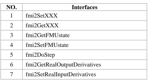
[image:2.595.175.421.308.441.2]The FMI standard has developed a series of standardized interfaces to ensure that the co-simulation can be performed efficiently and correctly. The main interfaces are shown in Table 1.
Table 1. Main interfaces in fmi co-simulation.
NO. Interfaces
1 fmi2SetXXX 2 fmi2GetXXX 3 fmi2GetFMUstate 4 fmi2SetFMUstate 5 fmi2DoStep
6 fmi2GetRealOutputDerivatives 7 fmi2SetRealInputDerivatives
1) fmi2SetXXX
This series of functions is used to set the value of the variable in the model. The value types include real number, integer, boolean, and string. The corresponding specific functions are fmi2SetReal, fmi2SetInteger, fmi2SetBoolean, fmi2SetString.
2)fmi2GetXXX
This series of functions is used to get the value of the variable in the model. The value type and the corresponding specific function are the same as the function fmi2SetXXX.
3) fmi2GetFMUstate
The current value of all state variables of the model is copied for saving, and then all state variables can be rolled back to this moment during simulation.
4) fmi2SetFMUstate
Rolls back all state variables to the state at a specific time. 5) fmi2DoStep
The model starts simulation until the next communication point, ie the model’s simulation clock advances one communication step.
6) fmi2GetRealOutputDerivatives
Get the derivatives of the output variables as the input for coupling model. 7) fmi2SetRealInputDerivatives
Set each order derivative of the input variable at the current communication point so that the input value at each time can be obtained by interpolation in the communication interval.
Approach for FMI Co-Simulation
interval between the two communication points called macro-step size or communication step size, denoted as H ).
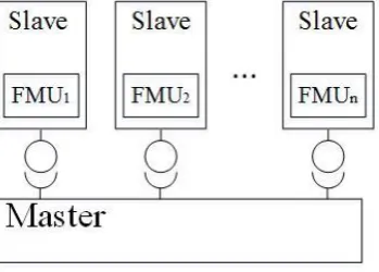
FMI co-simulation uses the Master-Slave framework, as shown in Figure 1. The master controls the scheduling of simulation, the data exchange, and the clock synchronization between models by master algorithm. The Slave is responsible for loading the subsystem (FMU) and executing the simulation. There is no data exchange between slaves. But data exchange can only be controlled by the master. This reflects the importance of the master algorithm in co-simulation.
The steps of FMI co-simulation are as follows:
1) Subsystem loading and initialization, set the current simulation clock tc as the start time of simulation;
2) Call function fmi2GetXXX to collect output values of all subsystems, and call function fmi2GetRealOutputDerivatives to collect derivatives of the output if necessary;
3) Call function fmi2SetXXX to distributed the output value obtained in step 1 to the subsystems as the input value at time tc in accordance with the coupling relationship between the subsystems, and then synchronize the simulation clocks of subsystems;
4) Call function fmi2DoStep to command subsystems to simulate until next communication point is coming, and the current simulation clock updates by tc=tc+H;
[image:3.595.213.388.326.451.2]5) Check if the end time of the simulation is reached. If yes, then stop; otherwise skip to step 2.
Figure 1. Master-slave framework.
Dynamic Selection of Extrapolation Functions
Selection Strategy
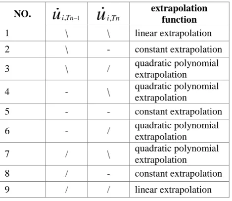
In the process that subsystems simulate independently, since no data exchange is involved, the inputs of subsystems are usually obtained by extrapolation. To avoid additional time consumption, commonly used extrapolation functions are some simple functions which include: constant extrapolation, linear extrapolation, and quadratic polynomial extrapolation. However, the existing researches mainly adopt a single extrapolation function. Although this strategy is simple, it cannot adapt to the different variability of the system at different time periods.
In order to overcome this shortage, this paper uses a method of dynamically selecting an extrapolation function. In this method, the data exchanged between subsystems at each
communication point is not only the input value u, but also its derivative
u
.u
i Tn, denotes thederivative of input u at communication point Tn. If
u
i Tn, ≤ -0.2, we use symbol “\” to representsits variability ; if -0.2 ≤
u
i Tn, ≤ 0.2 , we use symbol “_” to represents its variability; and if 0.2 ≤,
i Tn
u
, we use symbol “/” to represents its variability. Then in the communication intervalTable 2. Selection table of extrapolation function.
NO.
u
i Tn, 1u
i Tn, extrapolation function1 \ \ linear extrapolation
2 \ - constant extrapolation
3 \ / quadratic polynomial
extrapolation
4 - \ quadratic polynomial
extrapolation
5 - - constant extrapolation
6 - / quadratic polynomial
extrapolation
7 / \ quadratic polynomial
extrapolation
8 / - constant extrapolation
9 / / linear extrapolation
Implementation based FMI
To implement above method, we should implement the function fmi2DoStep in FMI standard as follow: at the beginning of the function, the extrapolation function should be selected according to Table 2, and before each step of simulation, the input value is calculated according to the selected extrapolation function. Then start the simulation.
Variable Macro-step Size
Although the dynamic selection of extrapolation function can effectively reduce the error caused by the extrapolation, it is obviously not completely eliminated. This error dominates the error of the whole subsystem[3]. And the greater the communication step size H, the greater the error caused; the smaller the H, the smaller the error. When H is equal to h(micro-step size ), the additional error will not exist. Therefore, in order to ensure that the subsystem can converge during the co-simulation process, the size of the communication step needs to be controlled.
First, the value of the error needs to be estimated, which can be done by Richardson extrapolation.
Richardson Extrapolation
The basic idea of Richardson extrapolation is as follow:
Assume that function D can be discretized into D (h), h donates step size:
p qDD h ah bh
(1) With p, q as the order of the reminder term, and p < q.
At the same time, function D can be also discretized into D (h2) with new step size h2:
2 2 2p q
DD h ah bh (2) Then, if we want to eliminate the term hp , we can carry out with eq.1 and eq.2 by
2
1 (h )p 2
h
2 2 1 1 1 q p q h b h D h rD hD h r r
(3)
Eq.3 can be briefly noted as
* * q
DD h b h
, D H( ) has replaced D H( ) as a new approximation of function D. Because it has a higher order of error term thanD H( ), it has higher accuracy. This is Richardson extrapolation’s contribution.
Macro-Step Size Control
The fact that co-simulation cause the additional error is that the subsystem adopts an extrapolation method to obtain the input value. In the communication interval
T Tn, n1
,the error estimation ofinput which obtained by polynomial extrapolation can be[4] :
1
0 2 1 ! k k n n l l K u T
u t u t t T
k H
( ) (4)
With real input function u t
, approximate function u t
. According to the error algorithm, wecan get error estimation of output y T
n 1
y Tn 1
at tTn1: Tn H. Then we can followRichardson extrapolation to calculate the actual value of error. First, subsystem should be simulated
twice with communication step size H Tn Tn H Tn 2H , and get output y T( n 2)
; then
subsystem need to be rolled back and be simulated with communication step size 2H:
2
n n
T T H
, and get output y T( n 2)
. After that, the actual value of error can be get by[5]:
2 1
2=
1 2
n n
k
y T y T
EST
(5) Where k is the order of polynomial extrapolation function. Assuming there are m outputs for the subsystem, each error of output can be calculated according to eq.5, notedESTj. Then we consider
the error indicator[6]:
2 1 2 1 m j j j
j j n
EST ERR
m
ATOL RTOL y
(6) Where ATOL is Absolute Tolerance, RTOL is relative Tolerance. A communication step H is accept, if ERR≤1; when ERR > 1, then the estimated error was too large and the communication step has to be repeated with a smaller step size. A smaller and optimal step size can be2 1 1 opt k H H ERR
Implementation Based FMI
[image:6.595.180.416.171.461.2]The implementation of the above method mainly involves the rollback, and FMI has provided interfaces include fmi2GetFMUstate and fmi2SetFMUstate to support it. The implementation with FMI standard is shown as Table 3:
Table 3. Implementation of variable communication step size.
Pseudo code for variable communication step size based FMI
1. for each FMU
2.Call fmi2GetFMUstate
3. Set input at Tn
4.Call fmi2DoStep with step size H
5. Set input at Tn1
6. Call fmi2DoStep with step size H
7.Call fmi2GetReal to get y(Tn2) 8.Call fmi2SetFMUstate
9. Set input at Tn
10.Call fmi2DoStep with step size 2H
11. Call fmi2GetReal to get y T( n2) 12. Calculate ESTj by eq.5
13. end for each
14. Calculate ERR by eq.6
15. if ERR1
16. Calculate Hopt by eq.7
17. H Hopt
18. end if
Case Study
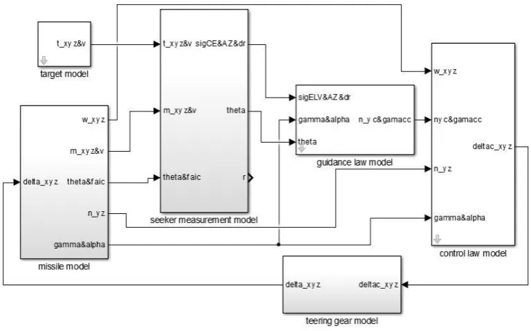
[image:6.595.104.488.531.770.2]This model consists of six sub-models: target model, missile model, seeker measurement model, guidance law model, control law model, and steering gear model. Each sub-model is built as FMU with function fmi2DoStep implemented in presented rule.
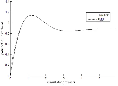
[image:7.595.197.405.189.341.2]The master algorithm was written in the VS2012 environment using FMI Library and developed by controlling communication step size. Simulate the system in Simulink environment and FMI environment respectively, set the ATOL of all outputs as 1e6, the RTOL is 1e4, the initial communication step is 0.1s. Select an output of the missile model (y-direction overload) as the observation. The comparison simulation results are shown in Figure 3.
Figure 3. Comparison of results.
Conclusions
In this paper, two error control methods are studied for the additional errors caused by the co-simulation: one is to improve the traditional extrapolation method, and the other is to control the communication step size. And apply these two methods to the latest standard-FMI. The case analysis results show that the simulation results in the FMI co-simulation using these two methods are in agreement with the results of the entire system simulation in Simulink, and demonstrate the effectiveness of the two methods.
References
[1] Pannu P., Andersson C., F. Hrer C., et al. Coupling Model Exchange FMUs for Aggregated Simulation by Open Source Tools. In proceeding of the 11th International Modelica Conference [C]. 2015.
[2] Nyl N.A., Henningsson M., Cervin A., et al. Control Design Based on FMI: a Diesel Engine Control Case Study [J]. Ifac Papersonline, 2016, 49(11): 231-238.
[3] Feki K.E., Duval L., Faure C., et al. CHOPtrey: contextual online polynomial extrapolation for enhanced multi-core co-simulation of complex systems [J]. Simulation Transactions of the Society for Modeling & Simulation International, 2016, 93(3):45-56.
[4] Li-Juan D., Qi-Yuan C. Numerical Methods [M]. Beijing: Higher Education Press, 2011.
[1] Hairer E., N. Rsett S.P., Wanner G. Solving ordinary differential equations [M].
Springer-Verlag, 2006.