Rectangular renormalization

J. Phys. A: Math. Gen. 18 (1995) 5469-5478. Printed in the UK

Rectangular renormalization

Jeffrey J Prentist and Bruce

S

Elenbogen$

t

Department of Natural Sciences, University of MichigawDearbo" Dearbom. MI 48128, USA

1 Department of Computer and Information Sciences, University of MichiganDearhm. Dearbom, MI 48128, USA

Received 6 June 1995

Abstract A generalized real-space renormalization scheme is developed for geometrical critical phenomena The renormalization group is parametrized by the standard length-scaling factor and a new redangular area-fraction factor. This rectangular renormalization scheme utilizes relatively small r e m g u l a r sublanices to effeaively renormalize large square lattices. With the area-fraction factor, one can systematically study rectangular generalizations of the conventional square-cell renormalization theories. Application to self-avoiding random walks yields critical descriptors that are comparable to, and in most cases better than previous results obtained from more complex renormaliration schemes.

1. Introduction

The renormalization-group theory is a 'vital tool to understanding critical phenomena. The real-space formulation of the renormalization group, by virtue of its simplicity and versatility, is widely used to study geometrical and thermodynamical systems [I]. Recent applications include surface phenomena [2], and self-organized criticality, such as diffusion- limited aggregation and sandpiles [3].

In

spite of its ubiquitous role in the theory of critical phenomena and scale-invariant systems, the practical implementation of real-space renormalization remains somewhat of an art, rather than a science. This is due to the uncontrolled nature of the approximations that are inherent to the real-space formulation. This is in Contrast to field theory, or momentum- space renormalization for which there exists a small parameter for systematically controlling a perturbation expansion. In real-space renormalization, the& does not exist any natural small parameter or rigorous set of criteria to ascertain' a ptiori whether or not a given approximation will yield results that are accurate andfor convergent. For g e o m e ~ c a l critical phenomena defined on lattices, all the approximations involve some type of truncation to a finite lattice, together with a rule for renormalization of the degrees of freedom. In spite of these seemingly drastic approximations, it is fortuitous that one can obtain reasonable results for the critical behaviour, usually within 5% to 10% of the exact values. However, in order to improve the accuracy, one must rely on more intricate techniques and additional rules. This can add substantial complexity to the basic 'zeroth-order renormalization scheme. This higher-order complexity includes the use of 'additional couplings, transfer matrices, toroidal lattices, Monte Carlo algorithms, finite-size scaling and other extrapolation methods

to

extend the small lattice results

to

larger lattices [4].

It

is

unfohnate that this large addition of technical complexity is usually incommensurate with the small gain in numerical accuracy. As a further complication, there exits a fundamental pathology of the real-space

5470

renormalization-group theory that renders it problematic in certain cases [ I , 51. A peculiar inconsistency in the standard real-space renormalization theory of percolation has recently been uncovered

16,

71.

In this paper, we present a generalized real-space renormalization scheme for geometrical critical phenomena that contains some of the conventional schemes as special cases. This generalized or rectangular renormalization represents a simple zeroth-order renormalization scheme, free of the complexities that characterize the higher-order methodology. Application of rectangular renormalization to the self-avoiding random walk problem in two dimensions yields critical points and exponents that

are

accurate, stable and convergent.

In

particular, simple calculations on small rectangular cells can produce results that are better than those obtained using large square cells, multiple cell clusters, and other more sophisticated renormalization schemes.

J

J

Prentis and B

S

Elenbogen

2. Renormalization

Consider any geometrical critical phenomena where the connectivity of the fluctuating d e grees of freedom is the microscopic trademark responsible for the long-range correlations, or scale invariance. The prototype geometrical systems, or lattice statistics problems, that ex- hibit critical behaviour are the self-avoiding random walk and percolation. For concreteness, we shall take the self-avoiding random walk

on a

lattice to illustrate the renormalization.

The renormalization-group theory allows one to understand the critical behaviour by probing the system at different len& scales. The renormalization transformation is the equa- tion that exhibits the structure of the system at these different length scales. In the real-space realization of the renormalization group, the basic definition [I] of the renormalization map is

W’(s’) P ( S ‘ , S ) W ( S )

where W ( s ) is the statistical weight (Boltzmann factor) of a state s on the original lat- tice, and W’(s‘) is the statistical weight of

a

renormalized (coarse-grained) state s’ on the rescaled lattice. The rescaled lattice is isomorphic to the original lattice and has a larger lattice spacing. The projection matrix P(s‘,

s)

specifies how to project the object state s onto the image state s’. More specifically, P(s’, s) determines the conditional probability that s’ is the image of s under the renormalization. The only constraint imposed on the projection matrix is that it must satisfy

P(s’, s) = 1.

I’

This normalization condition insures that

the

partition function (sum-over-states)

is a

renormalization-group invariant:

-

-E

W ‘ ( S ’ )

= E

W ( S ) .

I‘

(2.3)

Hence average values (observable$) generated from the partition function will be identical in the object and image spaces.

For the purpose of formulating a generalized renormalization scheme, we classify current real-space renormalization schemes into two categories:

(i) ‘Single-state’ renormalization: the renormalization map is computed directly from (2.1) by focusing on one renormalized state s’ at a time and the corresponding weight

[image:3.451.91.373.53.177.2]

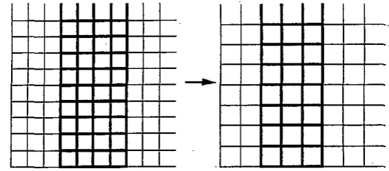
Figure 1. The mapping between the a-lauices, 10 x 10 + 8 x 8, and between the recrangular

w-lattices, IO x 5 -+ 8 x 4 (in bold), componding to a renormalization with length factor

b = ~5 a and area faccorf = f.'

(ii) 'All-state' renormalization. The renormalization map is computed from (2.3) by focusing on the set of all renormalized states simultaneously and the corresponding weight for the whole set of states. Note that this all-state weight is the sum-over-states of the single- state weights, or the whole~partition function. The cell-to-cell renormalization scheme

[SI

falls into this category.

In what follows, we formulate a~ more general renormalization scheme based

on

a partial partition function corresponding to a partial set of states on a rectangular sub-lattice. Consider a finite square lattice, denoted by Q, of size n x n, where n is the number of bonds on a side. Each bond is of length

e.

The rescaled square lattice, denoted

a'

, has a size n' x ni a n d a bond length~t'. The two microscopic length scales, and

e',

are related by the scaling factor b defined by

e'

= be (2.4)

where 1 c b c

w.

The original and the rescaled finite lattices, shown in figure 1, each represent one truncated cell of the infinite square lattice. This truncated square cell^ characterizes the single-cell renormalization schemes

[SI.

The collection of such square cells completely tile the infinite (parent) square lattice.

Now consider a rectangular sub-cell, denoted by w, of the original square cell, and the corresponding rectangular sub-cell, denoted w', of the rescaled.square cell (see figure 1).

To symbolically indicate that the rectangular sub-cell area is a fraction of the square cell area, we write

w = f Q and o'=

fa'

(2.5)

where f is the area fraction factor that can take on the values 0 c

f

g 1. We define the renormalization transformation by mapping the set of object states confined to the w-lattice onto the image states confined to the,"-lattice. Both object and image states should span the rectangular region by connecting the bottom edge to the top edge of the rectangle. This spanning rule is natural and common [4]. It preserves the essential long-range or macroscopic connectivity of the degrees of freedom.

Thus our renormalization is effectively a map between spanning states on a rectangular sub-lattice of size n x f n and spanning states on a rectangular sub-lattice of size n' x fn'.

5472

Given the additional freedom afforded by the area fraction factor

f,

that can assume a continuum of values between 0 and 1, one can explore a new class of renormalizations.

In more formal terminology, rectangular renormalization is defined by a projection matrix P(s’,

s)

that preserves the rectangular area spanned by the object state

s

and the image state s’. That is,

P(s’,

s)

takes on the value 1 if

s

and s‘ are confined to the same rectangular area, and is 0 otherwise. A less restrictive definition of the projection matrix is

J

J

Prentis and

B

S

Elenbogen

1 S E W

1

0 s g o

1

P(s’,

s)

=

$EO’

where s E o(s‘ E

o)

denotes those spanning states confined to, or completely embedded in the original rectangular lattice o (rescaled rectangular lattice

d).

Those spanning states that are not confined to the w-lattice are denoted by s

This choice of projection matrix S physically reasonable. In addition to preserving the long-range connectivity of the states, via spanning the rectangle, it also preserves the overall topology or coarse-grained shape of the states, by confining them to the same rectangular region. Each spanning state sweeps out a rectangular region as it spans the cell. The renormalization is a mapping between those spanning states whose bounding rectangular area is equal

to

or less than the area of o.

In other words, the rectangular o-lattice represents an ‘active zone’ and the complement of o is the ‘forbidden zone’. Spanning states with degrees of freedom that venture into the forbidden zone have zero projection to the active zone. Neglecting states that partially visit the forbidden zone is an approximation that is made for the sake of simplicity to avoid additional, arbitrary rules. It corresponds to zeroth-order ‘perturbation theory’. As the cell size increases, this approximation is expected to become more exact since these partially forbidden states represent a perturbation to the active states. The fraction of these perturbed states decreases as the cell size increases.

Our

results support this expected surface effect. The binary classification

of

macroscopic spanning~states into active-zone states

or

forbidden- zone states is a geometric analogue of Ising spin states in

a

magnetic system which can have the values of up or down. This is especially evident for the case

f

=

1

for which the active and forbidden zones have equal area. As far

as

the renormalization (projection matrix) is concerned, there exist only two kinds of spanning states: active or forbidden.

Given the area-preserving projection matrix, the rectangular renormalization transformation assumes the form

o.

W’(s’) = W ( s ) .

I’E f R’ ,€fR

This map follows from the basic renormalization equation (2.1) together with our definition of the rectangular projection matrix in (2.6). Note that we have also used

o

= fsl and

o’ = f

CY

in the sum-over-states to indicate the explicit dependence of thii map on the area fraction factor

f.

An alternative insight into the formal structure of rectangular renormalization can be found upon dissecting the invariant partition function relation in (2.3). Consider the decomposition of the sum-over-states into two partial sums:

It is instructive to compare the generalized, rectangular renormalization equation (2.7) to existing renormalization equations using the symbolism developed in this paper. The single- state (cell-to-bond, site decimation, cumulant) renormalization equation assumes the form

W'(3') = P(S',S)W(S). (2.9)

In

this expression, S2 represents any truncated lattice, including a single cell, a multiple-cell cluster, or a decimated lattice. The all-state (cell-to-cell) renormalization equation assumes the form

scn

(2.10)

When compared with the generalized renormalization equation (2.7), these other equations are characterized by j = 1, i.e. a sum over all states on the truncated lattice. An advantage of the all-state renormalization scheme is that it does not require a detailed specification of the projection matrix.

i n

general, the all-state renormalization schemes give more accurate results than the singlestate schemes

141.

This could be due to the fact that by only focusing on a single renormalied state, the invariance of the whole partition function is more easily violated.

3. Application to self-avoiding random walks

We apply rectangula renormalization to the self-avoiding random walk in two dimensions. This critical system serves as a paradigm for geometrical critical phenomena. For a self- avoiding random walk of N steps, the critical behaviour is characterized by the scaling of the multiplicity function (entropy) and the average size (correlations) of the walks for large

N:

where Z is the total number of walks and

R

is the root-mean-squared end-to-end distance of the walks. The critical exponents y and U determine the universal power law divergences,

while the lattice connective constant p determines the effective coordination number of the lattice. The critical descriptors, p and U, can be obtained from the real-space renormal- ization map in the usual way

[SI. In

the grand canonical statistics, each nearest-neighbour step of the object walk is weighted with a fugacity

K,

and each step of the image walk is weighted with

K'.

To maintain the simplicity of our scheme, we do not consider ad- ditional weights associated with steps beyond nearest-neighbour. Also for simplicity,

we

adopt the standard comer rule [8] for spanning the cell. Given the grand canonical statisti- cal weight W ( s ) = K N associated with each N-step walk, the rectangular renormalization equation (2.7) becomes a one-dimensional polynomial map parametrized by the length scal- ing factor b and the area fraction factor j . We denote this map by K & ( K ) . The non-trivial fixed point

K;,

of this nonlinear map and the eigenvalue hbf of the linearized map determine the critical descriptors according to

1

pbf =

-

where

K&

= K'(K;,) (3.3)

G I

In b dK'

vbf = -. where

A&

=

-(K&).

In Ab, dK (3.4)

The results for the critical point

K*

and the critical exponent U are displayed in tables 1-6

5474

J J Prentis and

B

S

Elenbogen

Table 1. The critical poini and exponent for area fnction f =

4.

n' x In'

"

x

4.

2 x 1 4 x 2 6 x 3 8 x 4 4 x 2 K' 0.4656

Y 0.7153 6 x 3 K* 0.4422 0.4235

U 0.7225 0.7322 8 x 4 'K 0.4286 0.4148 0.4072

U 0.7271 0.7363 0.7420

IO x 5 K* 0.4198 0.4090 0.4029 0.3989

Y 0.7300 0.7388 0.7440 0.7466

Table 2 The critical poid and exponent for area fnction f =

i.

"1 x :a'

n x + n 3 x 1 6 x 2 9 x 3 6 x 2 K* ~~ 0.4656

Y 0.7153

9 x 3 K' 0.4406 0.4206

Y 0.7241 0.7364

12 x 4 K' 0.4265 0.4119 0.4042

Y 0.7291 0.7404 0.7460

Table 3. The critical point and exponent for area fnction f =

$.

n' x $2

n x $n 4 x 1 8 x 2 8 x 2 K" 0.4656

Y 0.7153

1 2 x 3 K. 0.4398 0.4191

Y 0.7249 0.7386

Table 4. The critical Doini and emonent for area fraction f =

j.

n x a n 5 x 1 1 0 x 2 1 0 x 2 K' 0.4656

Y 0.7153

1 5 x 3 K' 0.4393 0.4182

Y 0.7253 0.74W

iown numerical estimate of

'

K

= 0.379 052

I

as

b --f 00 (down a column

of

the table) or as b + 1

11

and the exact value of U =

$

121

across a row or down the diagonal of the tablej. This behaviour as a function of the leng 1 scaling factor b for different area

fractions

f

is

a

generalization of the 6-dependence observed

in

the

conventional square-cell (f = 1) renormalization schemes

[SI.

[image:6.453.114.389.42.548.2] [image:6.453.114.336.66.281.2]

[image:7.451.55.406.61.551.2]

Table 5. The critical point and exponent for area fraction f =

i .

n' x ;d

n x i n , 6 x 1 1 2 x 2 1 2 x 2 'K 0.4656

Y 0.7153 1 8 x 3 ~ 'K 0.4390 0.4176

[image:7.451.65.367.64.325.2]

Y 0.7257 0.7408

Table 6. The critical point and exponent for area fractions f =

$

and f =

a.

n ' x fn'

n x fn 3 x 2 4 x 3 6 x 4 K' 0.4177

v 0.7324 8 x 6 K' 0.4036

"

0.7400

Table 7. Critical descriptors in the parameter space (b, f ) of the rectangular renormalization group. For each length scaling factor b ~ m d area fraction factor f, the critical point and

exponent are displayed. The first four rows represent single-sme (generalized cell-ro-bond) renormalizations. The last four rows represent all-state and pmial-state (generalized cell-to-

cell) renormalizations. The fin1 a l u m (f = 1) corresponds to the conventional square-cell renormalization scheme.

f

L _I

2 7 5

j

6

1 I

b 1

611 K' 0.4202

"

0.7258

511 K* 0.4264 0.4198 V 0.7241 0.73M)

411 K' 0.4348 0.4286 0.4265 V 0.7217 0.7271 0.7291

311 K' 0.4468 0.4422 0.4406 0.4398 0.4393 0.4390 V 0.7187 0.7225 0.7241 0.7249 0.7253 . 0.7257 312 K' 0.4319 0.4235 0.4206 0.4191 0.4182 0.4176

"

0.7224 0.7322 Or7364 0.7386 0.7400 0.7408 413 K' 0.4160 0.4072 0.4042

"

0.7307 0.7420 0.7460 514 K' 0.4068 0.3989

"

0.7360 Oi7466

615, K * 0.4011

"

0.7389

parametrized by the length factor b and the area factor f., The critical point

K&

and the critical exponent vb, are displayed for each point ( b , f). Note that the first column of

table 7, which corresponds to the special case f = 1, lists the critical results obtained from the standard square-cell renormalization scheme

[SI.

The overall trend of the data in this table indicates that optimal results are obtained from renormalizations characterized by

5476

exponent improve

as

the area factor f decreases. By fixed b in table 7, we mean fixed horizontal size of the rectangular cells, i.e. fixed m and m' for the mapping n x m -+ n' x m' where b = m/m' which is also equal to

nln'.

In rectangular renormalization, one has the freedom to choose not one, but two dimensions of the cell: the height and the width of the rectangle. The improvement of the critical results

as

f

-+

0

corresponds to renormalizing taller rectangles of fixed width.

In

particular, since n = m / f and n'

=

m ' / f , the height of the rectangle scales as 1/ f . Thus for the same 6 , the rectangle-to-rectangle renormaliza- tion

(f

+

1) produces better results than the conventional square-to-square renormalization

( f = 1). The faster convergence for rectangular lattices

as

b -+ 1 or b --f 00 is due to the

fact that for a given lattice width, the rectangular area is larger than the square area by the factor l / f . The other route to convergence for fixed b is via f -+ 1, which corresponds to using wider rectangles of fixed height. However, to produce a sxfficient amount of data that follows this route, one needs to use lattices of much larger area than the relatively small lattice areas used in this study. Thus, from a practical point of view, the f

+

0 route is much easier to simulate than the f -+ 1 route since there are exponentially fewer walks on tall rectangular lattices, such

as

15 x 3, as compared with the number of walks on wide rectangular (limiting square) lattices, ,such

as

15 x 15.

The difficult question of convergence for larger non-square lattices has 'been addressed in the phenomenological renormalization study of self-avoiding walks on infinite strips [13]. For the special case of infinitely tall rectangles and a scale factor of b = m / ( m

-

I), this study finds an overall rapid convergence to the exact values as b -+ 1, with monotonic convergence for strips with periodic boundary conditions. Thus it appears that the finite- size rectangles used in rectangular renormalization produce results that extrapolate to the exact values for a sequence of larger and larger rectangles. In contrast to this infinite-lattice study, we systematically investigate the effect of moving away from the standard square-cell renormalization to demonstrate the existence of simple and accurate finite-lattice schemes.

We are not aware of other small-cell renormalization calculations that have consistently achieved the level of accuracy of rectangular renormalization. For each renormalization, characterized by a different area factor f , we were able to obtain a value for the critical exponent in the range 0.74 < v c 0.75 from relatively simple calculations. Of particular note are the renormalizations corresponding to (b, f ) =

($,

+)

and

(2,i)

which yield

K' = 0.4042, v = 0.7460 and

K*

= 0.3989, U = 0.7466, respectively.

To illustrate this simplicity and accuracy of rectangular renormalization, we compare

our results with the best results obtained from other finite-lattice renormalization studies. The cumulant-like, majority-rule, multiplecell renormalization of [ 101 finds a result of

K' = 0.309, U = 0.712 from a second-order map consisting of five coupled equations

containing five coupling constants corresponding to different step weights with memory. The site-decimation, cluster renormalization of 1141 finds

a

result of K' = 0.4469, U =

0.7386 using a two-step approximation involving eight coupling weights, and a result of

K* =

0.3780, v = 0.7538 using a three-step approximation with twelve coupling weights. For the single-cell renormalization results, corresponding to the special case f = 1, see [SI. Some of the best results obtained from this square-cell renormalization study

are

K" = 0.4088, U = 0.7449 from a 6 x 6

+ 1

x 1 transfer matrix analysis;

K*

= 0.3759, v = 0.7443 using 5 x 5 -+ 4 x 4 toroidal cells; K" = 0.3807, v

=

0.7270 from a Monte Carlo simulation on 150 x 150 + 1 x 1 square cells. Note that the complexity

of

all the above renormalization schemes is significantly greater than that of rectangular renormalization. For a similar level of complexity, one should note the largest, pure and simple cell-to-cell renormalization that has been done, 6 x 6 -+ 5 x 5, gives a result of

K

'

= 0.4011, U = 0.7389 [SI. We have extended this square cell ( f = 1) result by

performing a 7 x 7

+

6 x 6 renormalization and find

K*

= 0.3971, U = 0.7402. This should be compared with OUI 10 x 5 4 8 x 4 result of

K

'

= 0.3989, U = 0.7466, since

both of these calculations involve similar computation time. It is interesting to note that the 7 x 7 + 6 x 6 square cell computation is slightly more complex (2% more computation time) than the 1 0 x 5 + 8 x 4 rectangular cell computation, in spite of the fact that the 1 0 x 5 = 50 total site area is slightly larger than the 7 x 7 = 49 total site area. This reflects the asymmetry in the entropy of the spanning walks as it depends on the horizontal and vertical dimensions of the finite lattice.. Thus, for a similar level of computational complexity (similar cell area), the pnre rectangle-to-rectangle renormalization gives a significantly better critical exponent than the pure square-to-square renormalization.

4. Discussion

Rectangular renormalization is a generalized renormalization. It is characterized by two scale factors: the length scaling factor b ~ =

t ' / e ,

and the area fraction factor f 5 wf Q .

Parametrized by b and f , there exists a family

of

renormalizations, 1 < b < CO &d

0 < f

<

1. that include some of the standard schemes as special cases. Geometrically, rectangular renormalization represents a mapping between spanning states on rectangular sublattices. Algebraically, it represents a partial partition function invariance.

The practical significance

of

rectangular renormalization lies in its simplicity and accuracy. It seems to be a high-efficiency renormalization scheme in that it produces the most accurate results for~a given amount of calculation. For the self-avoiding random^ walk problem, the results are comparable to, and in most cases better than results obtained from previous renormalization studies based on additional rules, higher-order approximations and/or more complex computations. As with square renormalization, there is no a priori justification for the use of the rectangular Cell .geometry of rectangular renormalization. However, given the rectangular results, it appears that large square lattices and intricate mapping rules are not necessary to achieve reliable results.

A~ new discovery is the effect of the rectangular area fraction on the critical descriptors. Unlike square renormalization (parametrized by b), rectangular renormalization (parametxized by b and f ) allows one independent control over both the vertical and the horizontal dimensions of the rectangular lattice. For fixed b, there exist two distinct optimal paths in (b, f ) pasameter space for which monotonic improvement occurs: the f

+

0 path. corresponding to increasing the height of rectangles of fixed width, i.e. ( m / f ) x m +

( m ' / f )

x

m', and the f

+

1 paih,~corresponding to increasing the width of kctangles of fixed height, i.e. n x f n + n' x fn'. For each of these paths, the improvement is due to increasing one of the dimensions of the.rectangle. The limiting critical values

K&,

vbo for f = 0, and

4.

ubl for f = 1, represent optimal values for a given b that become more exact as b approaches 1 or CO. For fixed

f,

we find that optimal renormalization occurs in the limit b

+

1 or b

+

CO, which is a generalization of the well known square-lattice? f = 1)

renormalization behaviour. This behaviour in the b- f plane provides insight into the basic anatomy of renormalization and practical criteria for designing a reliable approximation.

The accurate results that emerge from rather modest calculations are due to the effective large-lattice nature of rectangular renormalization. ~ The renormalization of the whole Q- lattice is accomplished by

focusing

on the smaller o-lattice. More specifically, although the actual calculation occurs

on

relatively small rectangular sub-cells: n x f n + n' x f n',

i.e. 12 x 4

+

9 x 3, the corresponding renormalization map refers to the original large square cells: n x n

-+

n' x n', i.e. 12 x 12 + 9 x 9, from which the rectangles are formed.

5478

of a class of walks embedded on the larger square lattice that project correctly under the renormalization. In other words, walks which span a rectangle seem to have the correct macroscopic connectivity and relevant topological information to produce a renormalization map that is a good approximation to the exact (iifinite square lattice) renormalization map. This indicates that the partial partition function defined on the rectangular cell contains the crucial coarse-grained, renormalization information. The whole partition function defined on the square cell is not necessary. This is perfectly consistent with the fundamental principles of the renormalization-group theory. According to these exact principles, although a renormalization map must leave the whole partition function invariant on all of state space (see equation (2.3)), the map itself is rigorously defined only between subsets of state space (see equation (2.1)). Walks confined to a rectangular sub-cell seem to provide a physically correct subset.

In a certain sense, our generalized renormalization scheme can be viewed as a hybrid scheme composed of the successful elements that characterize other real-space renormal- ization approximations. We have already discussed how rectangular renormalization, being based on a partial partition function, incorporates features from both the single-state and the all-state renormalization schemes. Other hybrid features are localization and spanning. In rectangular renormalization, the renormalization takes place between localized walks con- fined to a rectangular region within a single cell. The extent of the localization,

as

measnred by the size of the rectangle, is determined by the area fraction f . This localization is char- acteristic of the cluster renormalization schemes that include the site decimation

[9,

141 and the cumulant-like, multiplecell [lo] schemes. In rectangular renormalization, the cluster is simply a rectangle. The other feature of rectangular renormalization, that of spanning across a single cell, is characteristic of the well known cellular renormalization schemes

[8].

There are several natural extensions of rectangular renormalization as presented here. These include application to other critical phenomena, non-rectangular sub-cell geometries, three-dimensional ‘cylindrical renormalization’, perturbation into the forbidden zone, and analytic scaling in f and b. Preliinary studies of incommensurate rectangles (f

#

f’) indicate the expected result that the rectangular area should

be

preserved under the renormalization. It is hoped that rectangular renormalization will provide further insight into the nature of real-space renormalization and critical phenomena.

References

J J Prentis and B

S

Elenbogen

[I] Burkhardt T W and van keuwen J M I 1982 Real-Space Renormolirotion ed T W Burkhardf and J M J van

[Z] Cirillo E N M and Gonnella G 1995 J. Phys. A: Math. Gen. 28 867 [3] Vespignani A, Zapperi S and Pierronem L 1995 Phys. Rev. E 51 1711

[4] Stanley H E, Reynolds P I. Redner S and Family F 1982 Real-Space Renormalization ed T W Burkhardt

and I M J van b u w e n (Berlin: Springer) [5] Maninelli F and Olivieri E 1995 J. Stat. Phys. 79 25

[6] Ziff R M 1992 Phys. Rev. Leu. 69 2670

[7] Aharony A and Hovi I-P 1994 Phys. Rev. lea 72 1941 [SI Redner S and Reyoolds P J 1981 J. Phys. A: Math. Gen. 14 2679 [9] Shapiro B 1978 J. Phys. C: Solid Stare Phys. 11 2829

Leeuwen (Berlin: Springer)

[lo] Napi6rkowski M, Hauge E H md Hemmer F C 1979 Phys. Lert. 72A 193 [I I] Conwny A R, Enring I G and Gunmann A J 1993 J. P h y . A: Math. Gen. 26 1519

1121 Nienhuis B 1987 Phase Trmsitionr and Crirical Phenomena vol 1 1 ed C Domb and I L LebowiQ (New . .

York Academic)