Global Phase Synchronization for a Class of Dynamical Complex Networks with Time Varying Coupling Delays

Volume 2010, Article ID 295805,16pages doi:10.1155/2010/295805

Research Article

Global Phase Synchronization for a Class of

Dynamical Complex Networks with Time-Varying

Coupling Delays

XinBin Li and Haiyan Jing

Key Lab of Industrial Computer Control Engineering of Hebei Province, Yanshan University, Qinhuangdao 066004, China

Correspondence should be addressed to Haiyan Jing,[email protected]

Received 25 September 2010; Accepted 22 November 2010

Academic Editor: S. S. Dragomir

Copyrightq2010 X. Li and H. Jing. This is an open access article distributed under the Creative Commons Attribution License, which permits unrestricted use, distribution, and reproduction in any medium, provided the original work is properly cited.

Global phase synchronization for a class of dynamical complex networks composed of multiinput multioutput pendulum-like systems with time-varying coupling delays is investigated. The problem of the global phase synchronization for the complex networks is equivalent to the problem of the asymptotical stability for the corresponding error dynamical networks. For reducing the conservation, no linearization technique is involved, but by Kronecker product, the problem of the asymptotical stability of the high dimensional error dynamical networks is reduced to the same problem of a class of low dimensional error systems. The delay-dependent criteria guaranteeing global asymptotical stability for the error dynamical complex networks in terms of Liner Matrix InequalitiesLMIsare derived based on free-weighting matrices technique and Lyapunov function. According to the convex characterization, a simple criterion is proposed. A numerical example is provided to demonstrate the effectiveness of the proposed results.

1. Introduction

Over the recent decades, dynamical complex networks are increasingly used to model a variety of phenomena of nature in power system, biological system, traffic system, and so on1. Many of these networks exhibit complexity in the overall topological properties and dynamical properties of the network nodes and the coupled units. The complex nature of the networks has resulted in a series of important research problems. In particular, one significant and interesting phenomenon is the synchronization of all its dynamics.

machines. With the development of the modern industry and control technique, all kinds of rotating electrical machines play more and more important roles in industry. Therefore, the pendulum-like system is worth being researched not only of academic significant, but also of practical value.

Recently, the coupled pendulum-like systems attract more and more researchers’ attentions. Anticipating synchronization in a class of nonlinear dynamical systems is investigated in3. In4, the global asymptotical stability and generalized synchronization of phase synchronous dynamical networks composed of multiinput multioutput pendulum-like systems via linear interconnections are investigated. Of particular note is that the global synchronization of the dynamical complex network composed of the pendulum-like systems is different from that of the general complex networks. The global synchronization of the dynamical complex networks composed of the pendulum-like systems is defined as phase synchronization introduced in 4. But all of literatures above are not involving the coupling delays. However, time delay is unavoidably encountered, and it is the main cause of instability and poor performance of a system. Besides, the time-varying delays should be considered because they are more general than the constant cones. Thus, it is important and necessary to study the global synchronization of the dynamical complex networks composed of pendulum-like systems with time-varying coupling delays. In fact, the synchronization of the dynamical complex networks can be transformed into the global asymptotical stability of the corresponding error dynamical systems. In this paper, through studying the asymptotical stability of the corresponding error dynamical networks, several criteria guaranteeing the global phase synchronization of the dynamical network composed of multiinput multioutput pendulum-like systems with time-varying coupling delays are given. The effectiveness of the proved results is illustrated by a concrete example.

The rest of this paper is organized as follows. InSection 2, some preliminary results necessary for successive development are introduced.Section 3contains our main results. In this section, we give some criteria guaranteeing the phase synchronization of the dynamical complex networks composed of the multiinput multioutput pendulum-like systems with time-varying coupling delays. The effectiveness of the proposed results is illustrated with a numerical example given inSection 4, and a brief conclusion is given inSection 5.

The following notions are used in this paper. XT _{indicate the transpose for real X.}

X > 0 X < 0 meansX is a Hermitian and positivenegative definite matrix. IN, INn,

INm, In, and Im are N ×N, Nn×Nn, Nm×Nm, n× n, and m× m identity matrices,

respectively. I is an identity matrix with appropriate dimension. diag{X1, . . . , XN}, U⊗V

are defined by

⎛ ⎜ ⎜ ⎜ ⎝

X1 · · · 0

..

. . .. ...

0 · · · Xn

⎞ ⎟ ⎟ ⎟

⎠, U⊗V

⎛ ⎜ ⎜ ⎜ ⎝

u11V · · · u1mV

..

. . .. ...

un1V · · · unmV

⎞ ⎟ ⎟ ⎟

⎠. 1.1

2. Preliminaries

The nodes that compose a class of dynamical complex network can be described by following differential equation:

˙

xiAxi Bϕσi,

˙

σiCxi Dϕσi,

i1,2, . . . , N, 2.1

where variablesxi xi1, xi2, . . . , xinT andσi σi1, σi2, . . . , σimT denote the state variables.

A ∈ Rn×n_{, B ∈ R}n×m_{, C ∈ R}m×n_{, andD ∈ R}m×m _{are constant matrices. The continuously}

differentiable vector functionϕσi ϕ1σi1, . . . , ϕmσimT andϕl :R → RisΔl-periodic

with finite number of zeros on the interval0,Δl l 1, . . . , m. The system equation2.1

withΔ-periodicσiis called a pendulum-like system.

Proposition 2.1see2. If the solutionxitof the pendulum-like system2.1is bounded, then

the functions ϕlσilt (l 1, . . . , m), where σilt belongs to a solution of 2.1, are uniformly

continuous on0, ∞.

The validity of this assertion follows from the facts that ϕlσilt is locally Lipschitz

continuous andσ˙iltis bounded on0, ∞.

Lemma 2.2see2. Ifα:R → Rbelongs toL2_{0, ∞andβ:R → Rbelongs toL}2_{0, ∞,} then

τt

t

0

αt−τβτdτ −→0, t−→ ∞. 2.2

Lemma 2.3see2. Iff:R → Rand is uniformly continuous and isL20, ∞, then

lim

t→ ∞ft 0. 2.3

3. Main Results

The dynamical complex network considered in this study is composed by N identic pendulum-like nodes2.1with time-varying coupling delays, which could be described by the following equation:

˙

xit Axit Bϕσit N

j1

GijΓxjt−τt,

˙

σit Cxit Dϕσit, i1,2, . . . , N,

3.1

whereΓ∈Rn×n_{defines the coupling between any two nodes. If nodejis linked nodeii /j}

directly, thenGij Gji1; otherwise,Gij Gji 0i /j. The row sums ofGare zero, that

topology and coupling strength, andGis supposed to be irreducible. The time delay,τt, is a time-varying differentiable function that satisfies

0≤τt≤h,

˙

τt≤μ, 3.2

whereh >0 andμare constants.

Lemma 3.1 Wu 5. The eigenvalues of an irreducible matrix G Gij ∈ RN×N with

_N

j1,j /iGij−Gii(i1, . . . , N) satisfy the following properties.

i0 is an eigenvalue ofGassociated the eigenvector1,1, . . . ,1T.

iiIfGij ≥0for1≤i,j ≤N, andi /j, then the real parts of all eigenvalues ofGare less than

or equal to 0, and all possible eigenvalues with zero part are the real eigenvalue 0. In fact, 0 is an eigenvalue ofGwith multiplicity 1.

There exists an orthogonal matrixUsatisfyingUUT Isuch thatUTGU Λ, whereΛ is a diagonal matrix composed of eigenvalues ofG. According toLemma 3.1, it can be written as the following form:

Λ diag ⎛ ⎜ ⎜

⎝λ1, λ 2, . . . , λ2

m2

, λ 3, . . . , λ3

m3

, . . . , λq, . . . , λq

mq ⎞ ⎟ ⎟

⎠, 3.3

whereλ1 0 is the maximum eigenvalue of multiply 1, andλiis the eigenvalue of multiply

mii2,3, . . . , qsatisfyingm2 · · · mq N−1 and 0> λ2> λ3 >· · ·> λq.

Definition 3.2see4. The dynamical complex network model3.1is said to achieve global generalized phase synchronization if

lim

t→ ∞xit−xst2 0,

lim

t→ ∞σit−σst2 ς,

i1,2, . . . , N. 3.4

The sign · 2 here means the Euclidean norm, and ς is a constant value. xst, σst is

the solution of each single node which can be equilibrium points, periodic orbits, or even nonperiodic orbits with

˙

xsAxs Bϕσs,

˙

σsCxs Dϕσs. 3.5

From properties of the internal coupling matrixGgiven inLemma 3.1, we know that

N

3.5from3.1, we can get the following error dynamical system

˙

e1it Ae1it Bφe2it, σst N

j1

GijΓe1jt−τt,

˙

e2it Ce1it Dφe2it, σst,

i1,2, . . . , N, 3.6

withe1it xit−xst,e2it σit−σst, andφe2it, σst ϕe2it σst−ϕσst.

Sinceϕis a periodic function aboutσi,φe2it, σstalso has a period ofΔ. According to the

Kronecker product, system3.6could be written as follows:

˙

e1t IN⊗Ae1t IN⊗BΦe2t, σt G⊗Γe1t−τt,

˙

e2t IN⊗Ce1t IN⊗DΦe2t, σt,

3.7

where

e1

eT₁₁, . . . , eT_1NT, e2

e₂₁T, . . . , eT_2NT,

Φe2t φT_{e21t, σ}

st, . . . , φTe2Nt, σst

T

. 3.8

Under such circumstances, system 3.7 could be regarded as a pendulum-like system with state delay. Thus, the synchronization problem of the dynamical network 3.1 can be transformed into the global asymptotical stability problem of the corresponding error dynamical system.

Theorem 3.3. Suppose that there exist scalarsh > 0andμ, matricesPi P_iT > 0, Qi QT_i >0,

Ri RT_i > 0, Eij ET_ij > 0 (j 1,2),Ni N_iT₁ N_iT₂ N_iT₃ N_iT₄T,Si ST_i1 ST_i2ST_i3 ST_i4T,

Mi MiT1MTi2 MTi3 MTi4

T

and diagonal matrices κi, δi,εi with δi > 0,εi > 0 such that the

following inequalities are satisfied:

Π

⎛ ⎜ ⎜ ⎜ ⎜ ⎜ ⎜ ⎜ ⎜ ⎜ ⎜ ⎜ ⎜ ⎜ ⎜ ⎜ ⎜ ⎜ ⎜ ⎜ ⎜ ⎝

Π11 Π12 Π13 Π14 CT_ε

i hNi1 hSi1 hMi1 hATEi1 Ei2

∗ Π22 Π23 −N_iT₄ ST_i4 0 hNi2 hSi2 hMi2 hλiΓTEi1 Ei2

∗ ∗ Π33 −ST_i4−MT_i4 0 hNi3 hSi3 hMi3 0

∗ ∗ ∗ Π44 DT_ε

i 0 0 0 hBTEi1 Ei2

∗ ∗ ∗ ∗ −εi 0 0 0 0

∗ ∗ ∗ ∗ ∗ −hEi1 0 0 0

∗ ∗ ∗ ∗ ∗ ∗ −hEi1 0 0

∗ ∗ ∗ ∗ ∗ ∗ ∗ −hEi2 0

∗ ∗ ∗ ∗ ∗ ∗ ∗ ∗ −hEi1 Ei2

⎞ ⎟ ⎟ ⎟ ⎟ ⎟ ⎟ ⎟ ⎟ ⎟ ⎟ ⎟ ⎟ ⎟ ⎟ ⎟ ⎟ ⎟ ⎟ ⎟ ⎟ ⎠

<0, 3.9

2εi κiνi

∗ 2δi

whereΠ11PiA ATPi Qi Ri Ni1 N_iT₁ Mi1 M_iT₁,Π12 PiλiΓ−Ni1 N_iT₂ Si1 MT_i2, Π13 NT

i3−Mi1 MTi3−Si1,Π14 PiB N_iT₄ MT_i4 1/2CTκi,Π22 −1−μQi−Ni2−NiT2 Si2 STi2, Π23 −Si2 ST_i3−Mi2−N_iT₃,Π33 −Ri−Si3−S_iT₃−Mi3−MT_i3,Π44δi 1/2κiD 1/2DTκi,

νidiagνi1, . . . , νimwith

νil

_Δl

0

_Δl

0 φl

yilt, σslt

dyildσsl

_Δl

0

_Δl

0 φl

yilt, σsltdyildσsl

l1,2, . . . , m, 3.11

whereyt UT_⊗I

me2t y₁Tt, . . . , y_NTtT, andUis a selected orthogonal matrix satisfying

UT_{GU Λ, where Λ is defined as 3.3. Then the delayed pendulum-like system 3.7 with}

time-varying coupling delayτtsatisfying3.2is global asymptotic, stable and the corresponding dynamical network3.1achieves phase synchronization.

Proof. Recall the property of Kronecker product6

M⊗NG⊗D MG⊗ND, 3.12

where M ∈ Rk×m_{, N ∈ R}p×s_{,G ∈ R}m×n_{, andD ∈ R}s×q_{. Choose an orthogonal matrix U}

satisfyingUT_{GU Λ, whereΛis defined as the form of3.3. Let}

zt UT⊗In

e1t zT₁t, . . . , zT_NtT, yt UT_⊗I

m

e2t yT

1t, . . . , yTNt

T

. 3.13

Premultiplying two formulas of3.7byUT_⊗I

nandUT⊗Im, respectively, yields

˙

zt IN⊗Azt IN⊗BΦ

yt, σst

Λ⊗Γzt−τt,

˙

yt IN⊗Czt IN⊗DΦ

yt, σst

, 3.14

yielding

˙

zit Azit λiΓzit−τt Bφ

yit, σst

,

˙

yit Czit Dφ

yit, σst

, i1,2, . . . , N.

3.15

Introduce the new functions

Fl

yilt

φl

yilt, σslt

−νilφl

yilt, σslt, 3.16

therefore,

_Δl

0

Fl

yil

and the functionFlhas a mean value zero. We consider the following Lyapunov function:

V V1

m

k1

κik

yik

0

Fkτdτ, 3.18

where

V1zTitPizit

t

t−τtz

T

iαQiziαdα

t

t−h

zTiαRiziαdα

₀

−h

_t

t θ

˙

zT_iαEi1 Ei2z˙iαdα dθ.

3.19

By the New-Leibniz formula, we have

_t

t−h

˙

ziαdαzit−zit−h. 3.20

Then, in virtue of3.20, we have the following formulations for any matricesNi,Si,Miwith

appropriate dimensions:

Φ1zT_itNi1 zTit−τtNi2 zTit−hNi3 φT

yit, σst

Ni4

zit−zit−τt

−

_t

t−τtz˙iαdα

0,

3.21

Φ2zT_itSi1 zTit−τtSi2 zTit−hSi3 φT

yit, σst

Si4

zit−τt−zit−h

−

_t−τt

t−h

˙

ziαdα

0,

3.22

Φ3zTitMi1 zTit−τtMi2 zTit−hMi3 φT

yit, σst

Mi4

zit−zit−h

−

t

t−h

˙

ziαdα

0.

Calculating the derivative ofV1along the solutions of3.15and adding 2Φ1from3.21, 2Φ2

from3.22, and 2Φ3from3.23to it, we have

˙

V12zT_itPi

Azit λiΓzit−τt Bφ

yit, σst

zT_itQizit

−1−τ˙tzT_it−τtQizit−τt zT_itRizit−z_iTt−hRizit−h

hz˙T_itEi1 Ei2z˙it−

_t

t−h

˙

z_iTαEi1 Ei2z˙iαdα 2Φ1 2Φ2 2Φ3

≤2zTitPi

Azit λiΓzit−τt Bφ

yit, σst

zTitQixit

−1−μzTit−τtQizit−τt zTitRixt−zTit−hRizit−h

hz˙TitEi1 Ei2z˙it−

t

t−h

˙

ziTαEi1 Ei2z˙iαdα 2Φ1 2Φ2 2Φ3

ζTtΛ1ζt hz˙T_itEi1 Ei2z˙it−

_t

t−h

˙

zT_iαEi1 Ei2z˙iαdα

−2ζTtNi

t

t−τtz˙iαdα−2ζ

T_tS i

t−τt

t−h

˙

ziαdα−2ζTtMi

t

t−h

˙

ziαdα

ζTtΛ1 hAT_kEi1 Ei2Ak τtNiEi−11NiT h−τtSiE−i11STi hMiEi−21MTi

ζt

−

t

t−τt

ζTtNi z˙T_iαEi1

E_i−₁1N_iTζt Ei1z˙iα

dα

−

_t−τt

t−h

ζT_tS

i z˙TiαEi1

E−1

i1

ST

iζt Ei1z˙iα

dα

−

_t

t−h

ζTtMi z˙TiαEi2

E−_i21MT_iζt Ei2z˙iα

dα

≤ζTtΛ1 hAT_kEi1 Ei2Ak hNiE_i−₁1NiT hSiE_i−₁1STi hMiE−i21MTi

ζt

−

_t

t−τt

ζTtNi z˙TiαEi1

E_i−₁1N_iTζt Ei1z˙iα

dα

−

t−τt

t−h

ζTtSi z˙TiαEi1

E_i−₁1STiζt Ei1z˙iα

dα

−

_t

t−h

ζTtMi z˙TiαEi2

E−_i21MT_iζt Ei2z˙iα

dα,

where

ζTt zT

it zTit−τt zTit−h φT

yit, σst

,

Λ1

⎛ ⎜ ⎜ ⎜ ⎜ ⎜ ⎝

Λ11 Λ12 NT

i3−Mi1 MTi3−Si1 PiB NiT4 MiT4

∗ Λ22 −Si2 ST_i3−Mi2−N_iT₃ −N_iT₄ ST_i4

∗ ∗ −Ri−Si3−ST_i3−Mi3−MT_i3 −ST_i4−M_iT₄

∗ ∗ ∗ 0

⎞ ⎟ ⎟ ⎟ ⎟ ⎟

⎠,

Λ11PiA ATPi Qi Ri Ni1 NiT1 Mi1 MiT1,

Λ12PiλiΓ−Ni1 N_iT₂ Si1 MT_i2,

Λ22−1−μQi−Ni2−NiT2 Si2 STi2,

Ak A λiΓ 0 B.

3.25

SinceEil >0,l1,2, then the last three parts are all less than 0. So ifΛ1 hAT_kEi1 Ei2Ak

hNiE_i−₁1N_iT hSiE−_i11ST_i hMiE−_i21MT_i <0, then ˙V1<0.

Then,

˙

V V˙1

m

k1

κikFk

yikt

˙

yikt

_V˙₁ m

k1

κikφk

yikt, σskt

˙

yikt−κikνikφk

yikt, σskty˙ikt−εiky˙2_ikt

−δikφ2_k

yikt, σskt

εiky˙2_ikt δikφ2_k

yikt, σskt

.

3.26

In virtue of condition3.10of the theorem, there existδi0k>0 andεi0k>0 such that

κikνikφk

yikt, σskty˙ikt εiky˙2ikt δikφ2k

yikt, σskt

≥εi0ky˙2_ikt δi0kφ_k2

yikt, σskt

.

3.27

Thus, the following inequality is satisfied:

˙

Vt

m

k1

εi0kyik2t δi0kφ2k

yikt, σskt

≤_V˙_1t m

k1

κikφk

yikt, σskt

˙

yikt εiky_ik2t δikφ2_ik

yikt, σskt

.

Assuming that

Υt

m

k1

κikφk

yikt, σskt

˙

yikt εikσ_ik2t δikφ2_k

yikt, σskt

. 3.29

substituting the second equation of3.15into3.29, we have

˙

V1t Υt≤ζTtΛ1 hAT_kEi1 Ei2Ak hNiE−i11NiT hSiE−i11STi hMiE−i21MiT Λ2

ζt,

3.30

where

Λ2

⎛ ⎜ ⎜ ⎜ ⎜ ⎜ ⎜ ⎜ ⎝

CT_ε

iC 0 0 1

2C

T_κ

i CTεiD

∗ 0 0 0

∗ ∗ 0 0

∗ ∗ ∗ 1

2κiD 1 2D

T_κ

i DTεiD δi

⎞ ⎟ ⎟ ⎟ ⎟ ⎟ ⎟ ⎟ ⎠

, 3.31

andΛ1 hAT

kEi1 Ei2Ak hNiE−i11NiT hSiE−i11STi hMiEi−21MiT Λ2is equivalent toΠin

3.9by Schur complements. The inequality condition3.9of the theorem guarantees that

ζT_{tΛ1 hA}T

kEi1 Ei2Ak hNiE−i11NiT hSiE−i11STi hMiEi−21MTi Λ2

ζt<0. 3.32

Then, there exists a diagonal matrixρidiagρi1, ρi2, . . . , ρin,ρik>0,k1,2, . . . , n

ζT_{tΛ1 hA}T

kEi1 Ei2Ak hNiE−i11NiT hSiE−i11STi hMiE−i21MiT Λ2

ζt<−

m

k1

ρikz2_ik,

3.33

namely,

˙

Vzt, σt

m

k1

εi0ky˙2_ikt δi0kφ2_k

yikt, σskt

<−

m

k1

ρikz2_ik. 3.34

Hence,

Vt−V0≤ −

m

k1

t

0

εi0ky˙2_ikt δi0kφ2_k

yikt, σskt

dt−

n

k1

t

0

for all t ≥ 0. The function Vt is bounded because solutionszkt are bounded, and the

functionsFkτhave mean value zero. Therefore, from3.35, we have

_∞

0

φ2_kyikt, σskt

dt < ∞, 3.36

_∞

0

˙

y_ik2tdt < ∞, 3.37

_∞

0

z2_iktdt < ∞. 3.38

FromProposition 2.1, it follows that the functionsφyit, σstare uniformly continuous on

0, ∞. And from3.36andLemma 3.1, functionsφyit, σsttend to zero ast → ∞,

lim

t→ ∞φ

2

k

yikt, σskt

0. 3.39

Further, we have

yikt−→yikt, t−→ ∞, 3.40

whereφkyikt, σskt 0k 1,2, . . . , m. Let us now consider the the first equation of

system3.15. We can representzitin the form

zit eAtzi0

_t

0

eAt−sλiΓzis−τsds

_t

0

eAt−sBφ2_ikyiks, σst

ds. 3.41

From3.36,3.38, andLemma 2.3, we have

lim

t→ ∞

t

0

eAt−sBφik

yiks, σss

ds0,

lim

t→ ∞

_t

0

eAt−sλiΓzis−τsds0.

3.42

Furthermore, sinceAis Hurwitzian, the following conclusion is obtained:

lim

t→ ∞zit 0. 3.43

The conditions3.40and3.43show that every solutionzit, yitof the pendulum-like

system3.15converges to a certain equilibriumzieq0,yieqlyilwithφilyilt, σslt

0l1,2, . . . , m. Namely, the pendulum-like system3.7is global asymptotic stable.

addition, according to the convex properties of LMI7,q−3 groups of LMIs corresponding to λ3, . . . , λq−1 can be written as a linear combination of the tow groups of LMIs with the

second-maximumλ2and the minimum eigenvalueλq. Therefore, above criterion only needs

to examine three groups of LMIs corresponding to the largest, second largest, and the smallest distinct eigenvalues ofG, respectively. Furthermore, note that the system3.1withλ1 0

just corresponds to the synchronous manifold, which is not required to be verified. Hence, if

3.9and3.10hold forq2 andN, the nonlinear pendulum-like dynamical network will achieve phase synchronization.

Corollary 3.5. Suppose that there exist scalarsh > 0andμ, matricesPi PiT > 0,Qi QiT >0,

Ri RTi > 0, Eij ETij > 0 (j 1,2), Ni NiT1 NiT2 NiT3 NiT4

T

, Si STi1 STi2STi3 STi4

T

,

Mi MT_i1 MT_i2 MT_i3 M_iT₄T and diagonal matricesκi,δi,εi with δi > 0, εi > 0, such that the

following inequalities are satisfied:

⎛ ⎜ ⎜ ⎜ ⎜ ⎜ ⎜ ⎜ ⎜ ⎜ ⎜ ⎜ ⎜ ⎜ ⎜ ⎜ ⎜ ⎜ ⎜ ⎜ ⎜ ⎝

Π11 Π12 Π13 Π14 CT_ε

i hNi1 hSi1 hMi1 hATEi1 Ei2

∗ Π22 Π23 −NT

i4 STi4 0 hNi2 hSi2 hMi2 hλiΓTEi1 Ei2

∗ ∗ Π33 −ST_i4−MT_i4 0 hNi3 hSi3 hMi3 0

∗ ∗ ∗ Π44 DT_ε

i 0 0 0 hBTEi1 Ei2

∗ ∗ ∗ ∗ −εi 0 0 0 0

∗ ∗ ∗ ∗ ∗ −hEi1 0 0 0

∗ ∗ ∗ ∗ ∗ ∗ −hEi1 0 0

∗ ∗ ∗ ∗ ∗ ∗ ∗ −hEi2 0

∗ ∗ ∗ ∗ ∗ ∗ ∗ ∗ −hEi1 Ei2

⎞ ⎟ ⎟ ⎟ ⎟ ⎟ ⎟ ⎟ ⎟ ⎟ ⎟ ⎟ ⎟ ⎟ ⎟ ⎟ ⎟ ⎟ ⎟ ⎟ ⎟ ⎠

<0,

2εi κiνi

∗ 2δi

>0 i2, q,

3.44

whereΠ11PiA ATPi Qi Ri Ni1 N_iT₁ Mi1 M_iT₁,Π12 λiPiΓ−Ni1 N_iT₂ Si1 MT_i2, Π13 NT

i3−Mi1 MTi3−Si1,Π14PiB N_iT₄ MT_i4 1/2CTκi,Π22−1−μQi−Ni2−NiT2 Si2 STi2, Π23 −Si2 ST_i3−Mi2−NT_i3,Π33 −Ri−Si3−ST_i3−Mi3−MT_i3,Π44δi 1/2κiD 1/2DTκi,

and νi defined as the Theorem 3.3. Then, the dynamical network3.1with time-varying coupling

delayτtsatisfying3.2achieves phase synchronization.

4. Numerical Example

0 10 20 30 40 50 60 70 80

−8

−6

−4

−2

0 2 4 6 8

Time(s) x1

,x2

a

0 1 2 3 4 5

×105

−400

−200

0 200 400 600 800 1000 1200 1400 1600

Time(s)

σ

b

−4 −2 0 2 4 6

−8

−6

−4

−2

0 2 4 6 8 10

x1(t) x2

(

t

)

6

−

c

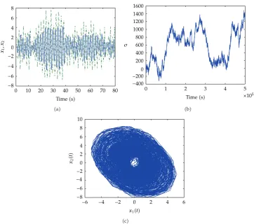
Figure 1:Simulation of each PLL node:x1,x2, andσand the phase plot betweenx1,x2, andσ.

The dynamical complex network3.1is composed of third-order PLL nodes with the following parameters:

A

−1 −2

5 1

, B

1

4

, C−2 2, D3, 4.1

and the nonlinear functionϕσi sinσi. The network topology parameters in4.1are

picked as

G

⎡ ⎢ ⎢ ⎢ ⎢ ⎢ ⎢ ⎢ ⎢ ⎣

−2 1 0 0 1

1 −2 1 0 0

0 1 −2 1 0

0 1 1 −3 1

1 0 0 1 −2

⎤ ⎥ ⎥ ⎥ ⎥ ⎥ ⎥ ⎥ ⎥ ⎦

0 5 10 15 20

−1.5

−1

−0.5

0 0.5 1 1.5 2 2.5 3

Time(s) e1j1

(

j

=

1

,...,

5

)

a

−2

−1

0 1 2 3 4

0 5 10 15 20

Time(s) e1j2

(

j

=

1

,...,

5

)

b

−4

0 2 4 6 8

0 5 10 15 20

Time(s) e2j

(

j

=

1

,...,

5

)

−2

c

Figure 2:The error variations in4.1:e1j1x11−xj1;e1j2x12−xj2;e2jσ1−σj, and j2, . . . ,5.

Assume that the inner-coupling matrix isΓ diag{1,1,1,1,1}. Eigenvalues of the coupling matrixGcan be calculated as

λ10, λ2−1.382, λ3−2, λ4−3.618, λ5−4. 4.3

The chaotic phenomenon of the state variablesx1andx2of the single PLL node is shown in

Figure 1. It is also observed that the phase variableσ is unbounded, so there is no chaotic phenomenon aboutσin plane phase space. However, chaotic phenomenon appears on the cylindrical surface of cylindrical phase space. This peculiar phenomenon to pendulum-like system is called the chaos on cylindrical surface9,10. Although the global asymptotical stability of pendulum-like system network model4.1may not be ensured, the global phase synchronization could be achieved. According toCorollary 3.5, whenh 0.2,μ 0.1, the LMIs3.44are feasible withλ2 −1.382,λ5 −4, that means for any time delay function

τtsatisfying 0≤τt≤0.2 and ˙τt≤0.1, the system4.1achieves phase synchronization. In the following, we give the simulation results for the case of the time delay functionτt

0.05 sint 0.051, and obviously τtsatisfies 0 ≤ τt ≤ 0.2 and ˙τt ≤ 0.1. The difference between state variablesxi1andximi1,2,m2, . . . ,5and the phase difference betweenσ1

andσmm2, . . . ,5are shown inFigure 2. And we can get that the state error variables are

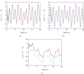
xi1

(

i

=

1

,...,

5

)

−3

−2

−1

0 1 2 3

0 5 10 15 20

Time(s)

a

xi2

(

i

=

1

,...,

5

)

−5

−4

−3

−2

−1

0 1 2 3 4 5

0 5 10 15 20

Time(s)

b

σi1

(

i

=

1

,...,

5

)

0 5 10 15 20

Time(s)

−20

−15

−10

−5

0 5 10

c

Figure 3:The synchronization variations in4.1ofxi1,xi2, andσi,i1, . . . ,5.

as defined byCorollary 3.5, which illustrated that the complex network4.1achieves phase synchronization. The changes of the synchronous statesxi1t,xi2t,σit i1, . . . , Nare

shown inFigure 3, from which we can also observe that the complex network4.1achieves the phase synchronization. All of these illustrate that result coincides with the theorem given above. Hence, the effectiveness of the proposed criterion has been proved.

5. Conclusion

studied by now. It shows the complexity of physical property in concrete systems even they are dichotomous. This also indicates that it is possible for the existence of chaotic attractors in pendulum-like systems.

Acknowledgments

This work is supported by National Natural Science Foundation of China under Grant no. 60874026 and Natural Science Foundation of Heibei province, China under Grant no. 07M007.

References

1 X. F. Wang, L. Xiang, and G. R. Chen,The Theory and Application of Complex Network, Tsinghua University, Beijing, China, 2006.

2 G. A. Leonov, D. V. Ponomarenko, and V. B. Smirnova, Frequency-Domain Methods for Nonlinear Analysis. Theory and Applications, vol. 9 of World Scientific Series on Nonlinear Science. Series A: Monographs and Treatises, World Scientific, River Edge, NJ, USA, 1996.

3 S. Xu and Y. Yang, “Predicting dynamic behavior via anticipating synchronization in coupled pendulum-like systems,”Journal of Physics A, vol. 42, no. 33, Article ID 335207, 15 pages, 2009.

4 S. Xu and Y. Yang, “Global asymptotical stability and generalized synchronization of phase synchronous dynamical networks,”Nonlinear Dynamics, vol. 59, no. 3, pp. 485–496, 2010.

5 C. W. Wu,Synchronization in Coupled Chaotic Circuits and Systems, vol. 41 ofWorld Scientific Series on Nonlinear Science. Series A: Monographs and Treatises, World Scientific, River Edge, NJ, USA, 2002.

6 C. W. Wu and L. O. Chua, “Application of Kronecker products to the analysis of systems with uniform linear coupling,”IEEE Transactions on Circuits and Systems I, vol. 42, no. 10, pp. 775–778, 1995.

7 S. Boyd, L. ELGhaoui, E. Feron, and V. Balakrishnam,Linear Matrix Inequalities in Systems and Control, SIAM, Philadelphia, Pa, USA, 1994.

8 Y. Yang, R. Fu, and L. Huang, “Robust analysis and synthesis for a class of uncertain nonlinear systems with multiple equilibria,”Systems & Control Letters, vol. 53, no. 2, pp. 89–105, 2004.

9 Z. Duan, J.-Z. Wang, and L. Huang, “Special decentralized control problems and effectiveness of parameter-dependent Lyapunov function method,” inProceedings of the American Control Conference (ACC ’05), vol. 3, pp. 1697–1702, Portland, Ore, USA, July 2005.