Time Dependent Discrete Network Design Problem

TIME-DEPENDENT DISCRETE NETWORK DESIGN PROBLEM

Liam O’BRIEN Ph.D. Student

Centre for Transport Research (TRIP) Dept. of Civil, Structural & Environmental Engineering

Trinity College Dublin Dublin 2

Ireland

Fax: +353-1-677 3072 E-mail: [email protected]

W.Y. SZETO Assistant Professor

Dept. of Civil Engineering National University of Singapore 1 Engineering Drive 2

E1A 07-03

Singapore 117576 Fax: +65-67791635

E-mail: [email protected]

Margaret O’MAHONY

Chair of Civil Engineering (1842) Centre for Transport Research (TRIP) Dept. of Civil, Structural & Environmental Engineering

Trinity College Dublin Dublin 2

Ireland

Fax: +353-1-677 3072

E-mail: [email protected]

Abstract: Over time transport networks are expected to remain highly reliable to ensure that users can experience smooth travel under both normal and abnormal traffic conditions. To design a reliable transport network properly it is necessary to take into account users reactions to incidents which cause disruption in different parts of the network over time. In order to design a reliable network to deal with such time-varying events it is necessary to capture the user’s route choice behavior under degraded conditions with the time dimension explicitly considered. Furthermore, for practical reasons, it is imperative that any improvement scheme be possible to implement. Therefore in this paper we formulate a time-dependent reliable discrete network design problem where the user’s behavior in route choice is modeled through the game theoretic approach. The ability of this model to design the critical links over time is demonstrated through two numerical studies under different budgets.

Key Words: Reliable discrete network design problem, Network reliability, Time-dependent risk-averse traffic assignment

1. INTRODUCTION

terrorist attacks. This requirement has meant that many early research efforts in the area have focused on developing measures for evaluating the network reliability. However very few studies have progressed to the next step that is, according to the general framework proposed in Du and Nicholson (1997), that the final goal of network reliability studies must be to provide useful information on network improvement programmes to transport policy makers. Therefore, progress in the area lies in the ability to use reliability studies to determine an optimal modification of the network. This problem (without uncertainty) is commonly known as the transport Network Design Problem (NDP).

The transport NDP is to improve a transport network in a manner that makes efficient use of resources, while also taking account of the travel choice behavior of potential network users or trip makers. Comprehensive reviews of the NDP have been carried out in the past, for example: Yang and Bell (1998). Traditionally the NDP is formulated as a bi-level problem with the upper level modeling the supply decisions undertaken by a planning authority to satisfy some objective, while the lower level models the travel choice decision of potential trip makers. Unlike the network supply, the potential trip makers are not directly under the influence of the planning authority but they react to the changes in transport networks by altering their travel decisions.

The NDP can be briefly classified into two catalogues: the Continuous Network Design (CNDP) and the Discrete Network Design Problem (DNDP). The former only includes continuous decision variables whereas the latter can contain both continuous and discrete decision variables. Moreover, the former takes the network topology as given and is concerned with optimizing the network parameters whereas the latter is concerned with the network topology in addition to optimizing network parameters. Indeed, the CNDP can be considered an approximation to the DNDP when the network topology is fixed, and has received considerably more attention in the literature (e.g. Chen et al. 2003; Chiou, 2005; Connors et al. 2005; Huang and Bell, 1998; Meng et al., 2001; Yang and Meng, 2000) possibly due to the computational benefits arising from using a continuous approximation to the discrete problem especially for large transport networks. Abdulaal and LeBlanc (1979) concluded from their computational results that a continuous approximate solution could be obtained at about 25% of the cost of obtaining an exact discrete solution. Despite the computational difficulty associated with the DNDP, there are still some examples in the literature, including the determination of new roadway links to be added to the network (e.g. Chen and Alfa, 1991; LeBlance, 1975), the bus network design problem (e.g. Wan et al., 2002), and the selection of pedestrianisation location (Wu et al., 2005).

Several researchers have tackled the NDP under uncertainty. Yin and Ieda (2002) analyzed the NDP with uncertain travel time. Waller and Ziliaskopoulos (2001) studied the problem of a dynamic NDP with demand uncertainty. Chen et al. (2003) introduced a mean-variance model to determine optimal tolls under the build-operate-transfer scheme with uncertain demand. Sumalee et al. (2006) developed a Reliable NDP (RNDP) considering demand and route choice variability. Their model allows the probability of user’s route choice to change in response to a change in the network following the concept of probit stochastic user equilibrium. Asakura et al. (2003) formulated a stochastic network design problem that provides a set of link investment patterns for the most reliable network with highest network performance under uncertain conditions. Other studies on reliable/stochastic NDP include Chootinan et al. (2005) and Chen and Yang (2004).

mainly caused by day-to-day demand variation and user’s behavior uncertainty. However, very few studies consider the user’s route choice behavior in a damaged network. This is due in part to the difficulty in collecting reliable behavioral data in a degraded network. One such approach which can model route choice behavior in a damaged network without relying on data is the game theoretic approach (Bell, 2000; Bell and Cassir, 2002; and Szeto et al., 2006).

The main idea behind the game theoretic approach is based on the notion of a fictitious game played between on the one hand users who seek minimum cost routes, and on the other hand, an evil entity or demon that seeks to maximize the total expected network cost to the users by damaging links in the network. The traffic assignment problem when formulated based on this approach, known as risk-averse traffic assignment, consists of two sub-problems: the user problem and the demon problem. The user problem describes the non-cooperative behavior of network users, whereas the demon problem describes the evil behavior in the sense of trying to cause maximum damage to the users. According to Bell and Cassir (2002) and Szeto et al. (2006), the game theoretic approach enjoys at least three advantages over the more conventional approaches. First, the game theoretic approach can determine links where the network users are the most vulnerable to link capacity degradation (i.e., links that give the most impact on the network users) under the assumption that the users are highly pessimistic or naturally very negative about the state of the road network. Second, this approach can provide normative measures of network reliability. Such normative measures are useful in pointing out the most vulnerable nodes (either origins or destinations), paths, and OD pairs in terms of encountering disruptions and travel time. Different designs may be compared on the basis of these measures. Third, statistical distributions for link performance (such as delay, travel time or capacity) are not required, unlike the more conventional approaches. This information is very often either absent or not accurate enough to be used.

One further problem with the above approaches to modeling the NDP under uncertainty and the RNDP is that they consider the network improvements to be continuous and to be one-off events which do not consider gradual network improvements or changing travel demands over a planning period. Recently Lo and Szeto (2004) posed the continuous NDP (CNDP) with the time dimension explicitly considered so as to allow for gradual improvements to the network and changing travel demands over a planning period. Their extension to include the time dimension is known as Time-Dependent CNDP (CNDP-T).

As mentioned already the computational advantages of using a continuous approximation to the discrete problem can be substantial. However the disadvantage is that it may be difficult in practice to translate the continuous solution into capacity improvements which can be implemented. In many cases this problem is exacerbated when the continuous solution determines relatively small improvements on a large number of links or many small improvements on the same link over many years. These small improvements are not realistic to implement due to the fact that road capacity is mainly determined by the number of lanes and lanes are indivisible. In this paper we avoid these problems by proposing a dependent formulation of the DNDP. However unlike the previous studies of both time-dependent NDP and the RNDP we adopt the game theoretic approach to modeling the lower level problem. Our resulting model allows us to explicitly consider network uncertainty in a time-dependent design framework with the capacity improvements as discrete variables. This new RNDP model is known here as the Time Dependent Reliable Discrete Network Design Problem (RNDP-T).

demands and the gradually upgraded network over the planning period but also more realistic and reliable capacity improvement schemes. The RDNDP-T is formulated as a single-level mathematical program which allows the use of existing nonlinear programming techniques for solutions. A number of examples are given to illustrate reliable network improvement strategies under a limited budget, demonstrate how only the most vulnerable links receive improvement and show how our method can design the critical links over time under an increased budget. In all examples important aspects of the RDNDP-T are highlighted such as the importance of introducing discrete variables to NDP over time and the importance of introducing the time dimension into the analysis. In all the numerical studies the Generalized Reduced Gradient (GRG) algorithm (Abadie and Carpentier, 1969) is adopted to obtain solutions.

The paper is organized as follows. Section 2 formulates the RDNDP-T model. Section 3 describes the numerical studies, while section 4 provides some concluding remarks and offers perspectives on future research.

2. FORMULATION

A general transportation network with multiple links, routes, and Origin-Destination (OD) flows over a planning period

[ ]

0,T is considered. The planning period is divided up into L

equal intervals. The length of each interval considered in this study is one year, but the formulation indeed does not pose any restriction on the length of each interval and the number of the intervals used, provided that their product is T. We adopt the following set of assumptions:

1. The potential demand growth over time is predicted perfectly.

2. Traffic assignment follows Wardrop’s first principle (Wardrop, 1952), and specifically in this study the route choice behavior of network users is described by the risk-averse traffic assignment formulated in Szeto et al. (2006).

3. We only consider the addition of indivisible facilities to the network topology and take the topology as given.

4. The functional form of the travel demand function remains unchanged over time although the parameters of this function do change over time.

5. The link costs and travel demand functions are separable.

6. The interest rates and inflation rates remain constant over time (for simplicity). 7. Only improvements costs are captured in the analysis, again for simplicity.

Lo and Szeto (2004) argue that the second assumption is reasonable since the length of each planning period is reasonably long so that the equilibrium condition is achieved within each period, and that each user has perfect information about the network state as is typically assumed in deterministic traffic assignment. Furthermore, in planning, the time duration between each design period is usually long enough for equilibrium to occur. The effect of the construction transition period, which is relatively short, is ignored. Most of the above assumptions are adopted to simplify the analysis and can be relaxed for future studies.

network is modified by constructing one “virtual” route to connect the origin and destination of each OD pair rs. There are Nτrs homogenous players between each OD pair rs in year τ ,

each of whom decides whether to travel, and if so, by which route. Each travel player is assumed to seek the minimum cost route whereas each non-travel player is assumed to select the sole artificially constructed “virtual” route. There is also a demon intent on causing maximum delays (and hence increased costs) to the travel players by damaging one and only one link on the whole network except the virtual links. This assumption can be easily relaxed in the future but we consider one demon just for the ease of illustration. Moreover, we assume that no player knows which link a demon will choose to damage, and no demon knows in advance which link a user may decide to use. Furthermore, each link is assumed to have only two costs depending on whether it is damaged or not. With this setting, we can formulate the risk-averse user equilibrium traffic assignment problem with elastic demands by applying the results in Nash (1951), Bell and Cassir (2002), and Szeto et al. (2006).

The proposed problem comprises two sub-problems: The user problem and the demon problem. The user problem can be viewed as a non-cooperative game, in which each homogenous player tries to select the route (including the virtual route) with minimum expected trip cost. This user problem can be approximated to deterministic traffic assignment when the number of homogenous players is large (Bell and Cassir, 2002). The first-order condition of deterministic traffic assignment for each time interval can be expressed as the following non-linear complementarity conditions:

( )

( )

d

min 0

rs rs rs

j jk k dk k

k k

h_τ g _τ q_τ g _τ q_τ

τ

⎡ ₋ ⎛ ⎞⎤₌

⎢ ⎜_⎝ ⎟_⎠⎥

⎣

∑

h

∑

h ⎦ , (1)

( )

( )

d

min 0

rs rs

jk k dk k

k k

g _τ q_τ g _τ q_τ

τ

⎛ ⎞

− _{⎜ ⎟}≥

⎝ ⎠

∑

h

∑

h , (2)

0 rs j

h_τ ≥ , (3)

( )

( )

d

min 0

rs rs rs rs

dk k

k

e_τ t_τ e_τ g _τ q_τ

τ

⎡ ₋ ⎛ ⎞⎤₌

⎢ ⎜_⎝ ⎟_⎠⎥

⎣

∑

h ⎦ , (4)

( )

( )

d

min 0

rs rs rs

dk k

k

t_τ e_τ g _τ q_τ

τ

⎛ ⎞

− _{⎜ ⎟}≥

⎝

∑

h ⎠ , (5)

0

rs

e_τ ≥ , (6)

where rs j

hτ is the flow on route j in year τ ; h is the route flow vector; grsjkτ

( )

h represents the

cost of route j between OD pair rs in scenario k in year τ based on the flow vector h; dτ is the minimum expected travel cost route between OD pair rs in year τ ; q_kτ is the probability of scenario k occurring in year τ ; e_τrs is the flow on the virtual route between OD pair rs in year τ satisfying the flow conservation:

rs rs rs

j j j

eτ =Nτ −

∑

δ hτ , (7)

whereN_τrsdenotes the total number of potential homogenous network players between OD

pair rs in year τ ; t_τrs

( )

e_τrs is an increasing virtual route travel cost function for each time

Conditions (1)-(3) are the time-dependent non-linear complementarity conditions for the routes on the network, excluding the virtual routes. According to (3), flows must be non-negative, implying that route j between OD pair rs in year τ can carry flow ( rs 0

j

h_τ > ) or carry no flow (hrs_jτ =0). If route j connecting OD pair rs in year τ carries flow (hrs_jτ >0), according to (1), the corresponding expected route travel cost between OD pair rs in year τ ,

( )

rs

jk k

k

g _τ q_τ

∑

h , must be equal to the minimum expected travel cost

( )

d

min _dkrs _k

k

g _τ q_τ τ

⎛ ⎞

⎜ ⎟

⎝

∑

h ⎠

between OD pair rs in year τ , as the term in the square bracket in (1) must equal zero. If route j connecting OD pair rs in year τ carries no flow (hrsjτ =0), the corresponding

expected route travel cost between OD pair rs in year τ must be greater than or equal to the minimum expected travel cost between OD pair rs in year τ based on (2).

Similarly, conditions (4)-(6) are the non-linear complementarity conditions for the virtual routes in each time slice. According to the non-negativity condition (6), flows on the virtual route must be non-negative in each year of the planning period. If the virtual route between OD pair rs in year τ carry carries flow (e_τrs >0), according to (4), the corresponding route

travel cost t_τrs

( )

e_τrs in year τ must be equal to the minimum expected OD travel cost

( )

d

min rs

dk k

k

g _τ q_τ τ

⎛ ⎞

⎜ ⎟

⎝

∑

h ⎠ between OD pair rs in that year. If the virtual route in year τ carries no

flow (e_τrs =0), the corresponding route travel cost in year τ must be greater than or equal to the minimum expected OD travel cost between OD pair rs in year τ by the definition of (5).

The demon problem describes the objective of the demon. The demon seeks a mixed strategy to maximise its own individual expected pay-offs or the total expected network cost to the users. The problem can be written for each time interval as the following non-linear complementarity conditions:

( )

( )

w

max rs rs rs rs 0

k _{jw j jk j}

j j

qτ g _τ h_τ g _τ h_τ

τ

⎛ ⎞

− =

⎜ ⎟

⎝

∑

h

∑

h ⎠ , (8)

( )

( )

w

max rs_jw rs_j rs_jk rs_j 0

j j

g _τ h_τ g _τ h_τ

τ

∑

h −

∑

h ≥ , (9)

0 k

q_τ ≥ , (10)

Where the probability q_kτ must satisfy:

1 0

k k

q_τ − =

∑

. (11)

and be non-negative as shown in (10) by definition, and grs_jkτ

( )

h follows the definition in (12).

Conditions (8)-(9) represent the necessary and sufficient conditions of the Nash equilibrium of a non-cooperative, mixed-strategy game for the demon (see Nash 1951). According to (8), if scenario k in year τ is selected (q_kτ >0), the maximum total expected network cost in

year τ ,

( )

w

max rs rs

jw j

j

g _τ h_τ

year τ , rs_jk

( )

rs_j

j

g _τ h_τ

∑

h , through the condition

( )

( )

w

max rs_jw rs_j rs_jk rs_j 0

j j

g _τ h_τ g _τ h_τ τ

⎛ ⎞

− =

⎜ ⎟

⎝

∑

h

∑

h ⎠ . If

scenario k in year in year τ , is not selected (q_kτ =0), the maximum total expected network cost in year τ must be greater than or equal to the total expected network cost in scenario k

in year τ according to (9).

2.2 The Definitional Constraints

The cost of route j between OD pair rs in scenario k in year τ , grsjkτ

( )

h , appeared in (1),

(2) and (4)-(5) is the total cost on every link that is on this route:

( )

( )

rs

jk ja ak a

a

g _τ h =

∑

δ t _τ v_τ , (12)

where δ_ja is 1 if link a is on route j, and 0 otherwise; t_akτ

( )

v_aτ denotes the flow-dependent

cost on link a in scenario k in year τ and is defined by the Bureau of Public Roads (BPR) function in (13) below:

( )

4 0

1 0.15 a ,

ak a a

ak

v

t v t

c τ τ τ τ ⎛ _{⎛ ⎞} ⎞ ⎜ ⎟ = + _{⎜ ⎟} ⎜ _{⎝ ⎠} ⎟ ⎝ ⎠ (13)

where t_a0 is the free-flow travel time of link a; c_akτ is the capacity of link a in scenario k in

year τ and v_aτ is the link flow in year τ . Both c_akτ and v_aτ are defined in (14) and (15) respectively:

0

1

ak ak a ai

i

c c y

τ τ λ τ

=

⎛ ⎞

= _⎜ + _⎟

⎝

∑

⎠, (14)

rs

a ja j

rs j

v_τ =

∑∑

δ h_τ . (15)

In (14) 0

a

c is the initial undamaged capacity of link a in year; the summation term in (14) represents the total capacity enhancements of link a up to the period τ and when added to the initial undamaged capacity of link a denotes the link capacity in period τ after implementing the capacity enhancements and inclusive of period τ ; whileλ_akτ is a link-damage indicator which equals one if there is no link-damage to link a in scenario k in year τ and equals 0.5 if there is damage to link a in scenario k in year τ . Equation (15) states that the link flow in year τ is simply the sum of the route flows using that link in year τ .

The travel cost tτrs

( )

eτrs on the virtual route which conceptually carries the non-travel demand

between OD pair rs in year τ and which is given in conditions (4)-(5), is assumed to satisfy:

( )

rs

rs rs rs e t e s τ τ τ τ

= , (16)

Where sτrs is an OD-specific parameter.

2.3 The Potential Travel Demand Function

the potential demands in successive periods. It represents the potential travel growth due to population growth, expressed as:

( )

1 , 1, ,

rs rs rs

N_τ =G N_τ− τ > ∀rs (17) Where Grs

( )

. is the potential demand function of OD pair rs. The potential demand in year

τ is modeled here to depend only on the potential demand in the previous year and not on the traffic conditions. This assumption is adopted here merely to simplify the analysis and follows similar assumptions used in Lo and Szeto (2005). The potential demand function can be easily extended to include changes in land-use patterns or other local environment factors. For simplicity, this paper employs a linear potential demand function, defined as:

1 1 ,

rs rs rs

N_τ =N_τ− ⎡_⎣ +p ⎤_⎦ (18)

Where prs is the growth rate of potential demand between OD pair rs.

2.4 Design Constraints

For practical reasons such as, for example, the unavailability of development land in urban areas, there is often an upper bound on the amount of capacity expansion that a highway link can undergo. Furthermore, in practice capacity depends on the number of lanes and link widening is a result of the addition of indivisible lanes to the existing network topology. Therefore in this study we model the capacity expansions as the multiple of the capacity of one lane. We further constrain the model to return only non-negative values of capacity expansion since we do not consider capacity reduction here and in general it is rare in practice. Mathematically these constraints may be expressed as:

, , ,

ak a

c _τ ≤u ∀a k τ (19)

, 0, , ,

a

y _τ ≥ ∀aτ (20)

, 0, , 2 ,..., , ,

a

y _τ = l l ∀aτ (21)

Where l is the capacity of a standard lane. In equation (19) we constrain the design to be less than its maximum allowable capacity by limiting the total capacity to be less than its maximum allowable capacity ua. Condition (20) is the non-negativity constraint of capacity

enhancements while equation (21) constrains capacity enhancements to be the multiple of the capacity of a standard lane. For simplicity, l is taken as 500 without loss of generality.

2.5 Improvement Cost Functions and Budgetary Constraints

The annual improvement cost K_τ is computed by summing the corresponding improvement costs of all links.

( )

, , , ,

a a

a

K_τ =

∑

m _τ y _τ ∀τ (22)

Where:

( )

0

(

)

( )

,1

, , ,0 1 , , ,

a

b

a a a a a

m _τ y _τ =b t + j τ−1 y _τ ∀aτ, (23)

( )

. a

m _,τ is the time-dependent improvement cost function of link a in year τ with parameters

,0, ,1

a a

b b and inflation factor

(

1+ j

)

τ−1. Equation (23) describes how the improvement cost of a link is proportional to the capacity enhancement y_a,τand its length 0

,0

a a

The budgetary constraints can be expressed as:

1 1 1,

K +R =B (24)

1 , 1,

K_τ +R_τ =R_τ− +B_τ ∀ >τ (25) Where B_τ is the network improvement budget allocated by the government at the beginning

of year τ . The variable R_τ represents the cumulative allocated funds that have not yet been spent in year τ and are available for use at the beginning of year τ +1. Equation (25) states that the sum of the total cost of the improvements for year τ and the funds unspent or saved for the future years after τ is equal to the budget allocated by the government for year τ plus the funds saved from year 1 to τ−1. Equation (24) describes the beginning of the planning horizon, assuming that no funds were saved before the planning horizon. This set of recursive equations permits the modeling of various budget and expenditure scenarios. For example, if the government provides a lump sum only at the beginning of the planning horizon, then

1 0

B > and B_τ =0, τ >1. Then (24)-(25) can be reduced to K_τ B₁ τ

≤

∑

.

2.6 The Objective Function

For simplicity we adopt an objective function with a straightforward interpretation. We consider the minimization of expected total system travel cost (ETSTC). ETSTC describes the expected total travel time spent by users in the network converted to a monetary value and is very straightforward to compute given the link flows, damage probabilities, the value of time and a parameter to convert hourly flows to annual flows. Mathematically, it can be expressed as:

( )

(

)

(

a ak a k

)

,

rs a k

ETSTC n vτ t τ vτ qτ

τ

ψ

=

∑∑∑∑

(26)

where v_aτ is the link flow in year τ as given in equation (15); t_akτ

( )

v_aτ is the link travel time in scenario k in year τ given in equation (13); qkτ is the probability of scenario k occurring

in year τ . The product n v

(

_aτ

(

t_akτ

( )

v_aτ q_kτ

)

)

ψ is evaluated for every link in each scenario for each origin-destination pair rs in the network over the entire planning horizon.

2.7 The RDNDP-T formulation

The time-dependent reliable discrete network design problem (RDNDP-T) can then be formulated as:

( )

(

)

(

)

, , ,

min a ak a k

rs a k

ETSTC n vτ t τ vτ qτ

τ

ψ

=

∑∑∑∑

h y q e

subject to: time-dependent risk-averse traffic assignment constraints (1)-(11), definitional constraints (12)-(16),

potential travel demand function (17), design constraints (19)-(21),

improvement cost and budgetary constraints (22)-(25),

which follow, the RDNDP-T formulation is solved using the Generalised Reduced Gradient (GRG) algorithm proposed by Abadie and Carpentier (1969). The detailed algorithmic steps are described in Lo and Szeto (2004).

3. NUMERICAL STUDIES

In the following two examples, we illustrate a number of aspects: the design approach of the RDNDP-T model under different budgets, the selection and design of the vulnerable links over time, the necessity of considering the time dimension in the modeling approach and the importance of using discrete capacity improvement variables over time in reliable network design.

3.1 The RDNDP-T approach to designing the critical links over time under tight budgetary constraints

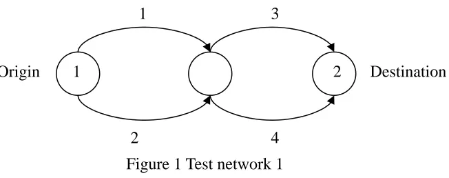
This example aims at illustrating the design approach of the RDNDP-T when only a small budget is provided by the government at the beginning of the planning horizon. The simple test network used to generate results is shown in figure 1 below and consists of one OD pair. The OD pair (1,2) connects node one (the origin) to node two (the destination) via four possible routes – route one which uses links one and three, route two which uses links one and four, route three which uses links two and three, and route four which uses links two and four. The following parameters which are chosen for illustrative purposes also apply:

Free-flow travel times: 0 0 0 0

1 2 4 10 minutes; 3 5 minutes

t = = =t t t =

Initial undamaged link capacity: c₁0 =c₂0 =c₃0 =c₄0 =4000 vph

Initial damaged link capacity: c10 =c20 =c30 =c40 =2000 vph

Demand parameters: N₁12 =4000 vph;p12 =0.075;s₁12 =s12₂ =s12₃ =s12₄ =s12₅ =10 vph per euro

Maximum allowable link capacity: u₁=6500 vph; u₂ =10000 vph; u₃ =u₄ =18000 vph Value of time:ψ =€60/hour

Factor to convert hourly flows to annual flows: n=8760

Improvement cost parameters: b_1,0 =€43,000/veh.; b_1,1=€1/veh.

Inflation rate: j=0.01

Design period:

[ ] [ ]

0,T = 0,5 years

This example considers the design strategies adopted by the RDNDP-T model under very 1

1

3

2

2

[image:10.595.132.458.591.720.2]

4

Figure 1 Test network 1

tight budgetary constraints. A very small budget of is given (B₁ =€5.38 x 10 ) and the results 8 are discussed in the following paragraphs.

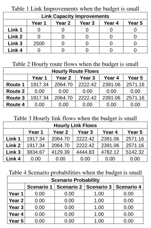
[image:11.595.147.449.192.646.2]

In this scenario the government provides a small budget as a lump sum at the beginning of the planning horizon. Under these conditions we expect that only the most necessary improvements to the network be carried out. Table 1 shows the link improvements for the entire planning period, table 2 and table 3 show the hourly route and link flows respectively, while table 4 shows the scenario probabilities.

Table 1 Link Improvements when the budget is small

Link Capacity Improvements

Year 1 Year 2 Year 3 Year 4 Year 5

Link 1 0 0 0 0 0

Link 2 0 0 0 0 0

Link 3 2500 0 0 0 0

[image:11.595.155.443.203.369.2]

Link 4 0 0 0 0 0

Table 2 Hourly route flows when the budget is small

Hourly Route Flows

Year 1 Year 2 Year 3 Year 4 Year 5

Route 1 1917.34 2064.70 2222.42 2391.06 2571.16

Route 2 0.00 0.00 0.00 0.00 0.00

Route 3 1917.34 2064.70 2222.42 2391.06 2571.16

Route 4 0.00 0.00 0.00 0.00 0.00

Table 3 Hourly link flows when the budget is small

Hourly Link Flows

Year 1 Year 2 Year 3 Year 4 Year 5

Link 1 1917.34 2064.70 2222.42 2391.06 2571.16

Link 2 1917.34 2064.70 2222.42 2391.06 2571.16

Link 3 3834.67 4129.39 4444.83 4782.12 5142.32

Link 4 0.00 0.00 0.00 0.00 0.00

Table 4 Scenario probabilities when the budget is small

Scenario Probability

Scenario 1 Scenario 2 Scenario 3 Scenario 4

Year 1 0.00 0.00 1.00 0.00

Year 2 0.00 0.00 1.00 0.00

Year 3 0.00 0.00 1.00 0.00

Year 4 0.00 0.00 1.00 0.00

Year 5 0.00 0.00 1.00 0.00

[image:11.595.162.434.522.638.2]

interesting to note that despite the improvements in capacity to link three, the demon still determines this to be the critical link in the network. This implies that the users are most vulnerable to failure on this link and requires a larger budget to lessen the impact of a failure. Finally we can also see that the capacity improvement of 2500vph is one that is possible to implement since it corresponds to the addition of five to new lanes to link three under our assumption that the capacity of one lane corresponds to 500vph. This emphasizes the advantage of using discrete capacity improvement variables.

According to table 1 the demon always selects link three in this setting since it attracts the most users and hence damage to this link results in the most users being affected. The capacity improvements selected under this limited budget will mitigate this effect somewhat but nonetheless this link remains the critical one due to the large number of users traveling on this link (see table 3).

This simple example demonstrates how the RDNDP-T determines that only the most vulnerable link is selected for link improvements under constrained resources.

3.2 The RDNDP-T approach to designing the critical links over time under a large budget

In this study we adopt the same network as in figure one and the same network and demand parameters as before but this time we provide a much larger budget than before (B₁=€6.44

9

x 10 ). We do not constrain the model to spend the entire budget with the result that only necessary capacity improvements are recommended. Table 5 shows the link capacity improvements for this particular case. As before, we can see that link three receives the most improvement since it is generally remains the link which is most vulnerable to failure. Furthermore the maximum allowable link capacity of link three is quite high which allows for this type of capacity expansion. Link two receives the second greatest capacity improvement since its maximum allowable capacity is much higher than link one’s and furthermore by the start of year three it is much wider than link one, thereby attracting more travel demand (see table 7) and hence further capacity enhancements. Link one receives the least capacity improvements since its maximum allowable capacity is smaller than link two’s and therefore the physical space is not there to expand the link any further.

[image:13.595.142.458.138.561.2]

capacity and fails to attract more users. However due to the large budget, the increases in demand, and having the space to do so, link three continues to expand in capacity thereby attracting more users to it. This is reflected in the scenario probabilities for these two years as link three is selected by the demon with a probability of almost one.

Table 5 Link capacity improvements under large budget

Link Capacity Improvements

Year 1 Year 2 Year 3 Year 4 Year 5

Link 1 0 2500 0 0 0

Link 2 0 3500 2500 0 0

Link 3 3000 3000 3000 1500 1500

Link 4 0 0 0 0 0

Table 6 Hourly route flows under large budget

Hourly Route Flows

Year 1 Year 2 Year 3 Year 4 Year 5

Route 1 1918.93 1969.10 1315.57 1886.77 2142.98

Route 2 0.00 0.00 0.00 0.00 0.00

Route 3 1919.22 2177.12 3155.08 2930.82 3047.42

Route 4 0.00 0.00 0.00 0.00 0.00

Table 7 Hourly link flows under large budget

Hourly Link Flows

Year 1 Year 2 Year 3 Year 4 Year 5

Link 1 1918.93 1969.10 1315.57 1886.77 2142.98

Link 2 1919.22 2177.12 3155.08 2930.82 3047.42

Link 3 3838.15 4146.21 4470.66 4817.59 5190.40

Link 4 0.00 0.00 0.00 0.00 0.00

Table 8 Scenario probabilities when budget is large

Scenario Probability

Scenario 1 Scenario 2 Scenario 3 Scenario 4

Year 1 0.01 0.01 0.98 0.00

Year 2 0.02 0.02 0.95 0.00

Year 3 0.03 0.30 0.67 0.00

Year 4 0.01 0.02 0.97 0.01

Year 5 0.00 0.00 0.99 0.00

[image:13.595.130.468.482.573.2]

4. CONCLUDING REMARKS

This paper proposed a time-dependent formulation of the reliable discrete network design problem by modeling the user behavior in route choice via the game theoretic approach. The resulting model allows us to explicitly consider uncertainty in the network design problem and does not rely on data on user behavior in a damaged network. The time-dependent framework of the RDNDP-T permits modeling of: time-dependent travel demands; capturing the gradually upgraded network over the planning period; the determination of optimal timing of project construction; project scale and phasing; determining the critical links and allowing these links to receive priority in the improvement scheme, thereby resulting in a reliable network design. By basing the network design on the expected travel costs of the users when confronted by supply uncertainty, this approach introduces improvements which cater for the worst case scenarios of network reliability. We formulated the RDNDP-T as a single-level optimization program, solved it through the GRG solution algorithm, and through numerical examples demonstrated how the model determines the critical links and how under different budgets the model prioritizes capacity enhancements which are practical to implement.

The results presented here are somewhat preliminary. Nevertheless, we believe the discussions and the proposed formulation have opened up some interesting future research directions. First, the proposed formulation of the RDNDP-T does not take into account multiple states of link damage since the sole demon is restricted to damaging only one link in each OD pair. Furthermore the sole demon can only damage each link by 50%. One worthy future study would be to model the RDNDP-T under multiple network demons whom can combine to damage the same links in the same day resulting in an even greater capacity reduction. This would allow many more operational states to be modeled and may produce the worst case scenario of network reliability. Second, the RDNDP-T model presented here restricts the investment money to be used solely for link widening. However, it may also be interesting in the future to consider the effect of using the budget to improve the physical robustness of the links, i.e., improving the structural toughness of the link against natural disaster. Third, the algorithm used here to generate solutions is a general-purpose algorithm and may not be best suited to handle the highly non-convex RDNDP-T. Further research is required to develop a suitable solution scheme to handle the discrete capacity constraints, particularly when we consider larger networks, and the non-convexity. Finally, the BPR function adopted here cannot accurately describe the realistic relationship between travel time and flow as the congested part of the flow density curve is not captured by the BPR function. Extending the proposed framework to consider the flow-density relation must be an interesting and important future research direction.

ACKNOWLEDGEMENTS

This research is sponsored by the start-up grant R-264-000-229-112 from the National University of Singapore and supported by the Programme for Research in Third-Level Institutions (PRTLI) administered by the Irish Higher Education Authority.

REFERENCES

the case of nonlinear constraints, in R.Fletcher (ed.), Optimization, New York: Academic Press, pp. 37-47.

Abdulaal, M.S. and Le Blance, L.J. (1979) Continuous equilibrium network design models, Transportation Research, Vol. 13B, 19-32.

Asakura, Y., Hato, E. and Kashiwadani, M. (2003) Stochastic network design problem: An optimal link investment model for reliable network, The Network Reliability of Transport: Proceedings of the 1st International Symposium on Transportation Network Reliability (ed M.G.H. Bell and Y. Iida), Pergamon, 245-259.

Bell, M.G.H. (2000) A game theory approach to measuring the performance reliability of transport networks, Transportation Research, Vol. 34B, No. 6, 553-546.

Bell, M.G.H. and Cassir, C. (2002) Risk-averse user equilibrium traffic assignment: An application of game theory, Transportation Research, Vol. 36B, No. 8, 671-681.

Chiou, S. W. (2005) Bilevel programming for the continuous transport network design problem, Transportation Research, Vol. 39B, No. 4, 361-383.

Chen, A. and Yang, C. (2004) Stochastic transportation network design problem with spatial equity constraint, In Transportation Research Record: Journal of the Transportation Research Record,Vol. 1882, TRB, National Research Council, Washington, D.C., 97-104. Chen, A., Subprasom, K., and Ji, Z. (2003) Mean-variance model for the

build-operate-transfer model under demand uncertainty, In Transportation Research Record: Journal of the Transportation Research Record, No. 1857, TRB, National Research Council, Washington, D.C., 93-101.

Chen, M.Y. and Alfa, A.S. (1991) A network design algorithm using a stochastic incremental traffic assignment approach. Transportation Science,Vol. 25, No. 3, 215-224.

Chootinan P., Wong S.C. and Chen A. (2005) A reliability-based network design problem. Journal of Advanced Transportation, Vol.39, No. 3, 247-270.

Connors, R., Sumalee A, Watling D. (2005) Equitable network design. Journal of Eastern Asia Society for Transportation Studies, Vol. 6, No. 1, 1382-1397.

Du, Z.P. and Nicholson, A.J. (1997) Degradable transportation systems: Sensitivity and reliability analysis. Transportation Research, Vol. 31B, No.3, 225-237.

Huang, H. J. and Bell, M. G. H. (1998) Continuous equilibrium network design problem with elastic demand: Derivative-free solution methods, Transportation Networks: Recent Methodological Advances (ed MGH Bell), Oxford: Pergamon, 175-193.

LeBlanc, L.J. (1975) An algorithm for discrete network design problem, Transportation Science, Vol. 9, No. 3,183-199.

Lo, H.K. and Szeto, W.Y. (2005) Time-dependent transport network design under cost-recovery. , Transportation Research B, tentatively accepted.

Lo, H.K. and Szeto, W.Y. (2004). Planning transport network improvement over time, Urban and Regional Transportation Modeling: Essays in Honor of David Boyce, Chapter 9, 157-176. Edited by D.H. Lee. Edward Elgar.

Meng, Q., Yang, H. and Bell, M.G..H. (2001) An equivalent continuously differentiable model and locally convergent algorithm for the continuous network design problem. Transportation Research, Vol. 35B, No. 1, 83-105.

Nash, J. (1951) Non-cooperative games, Annals of Mathematics, Vol. 54, 286-295.

Szeto, W.Y., O’Brien, L. and O’Mahony, M. (2006) Risk-averse traffic assignment with elastic demands: NCP formulation and solution method for assessing performance reliability, Networks and Spatial Economics, Vol. 6, 313-332.

Waller, S.T. and Ziliaskopoulos, A.K. (2001) Stochastic dynamic network design problem, In Transportation Research Record: Journal of the Transportation Research Record,No. 1771, TRB, National Research Council, Washington, D.C., 106-113.

Wan, K.H., Lo., H. and Yip, C.W. (2002) Optimal integrated transit network design, in Wang, C.P. et al. (eds.). Proceedings of the Seventh International Conference of the ASCE Applications of Advanced Technologies in Transportation, USA: American Society of Civil Engineers, pp. 736-743.

Wardrop, J. (1952) Some theoretical aspects of road traffic research, Proceedings of the Institute of Civil Engineers, Part II, 325-378.

Wu, Z.X., Lam, William H.K., Chan, K.S. (2005) Multi-modal network design: Selection of pedestrianisation location, Journal of Eastern Asia Society for Transportation Studies, Vol. 6, No. 1, 2275-2290.

Yang, H. and Bell, M.G.H. (1998) Models and algorithms for road network design: a review and some new developments, Transport Reviews, Vol. 18, No. 3, 257-278.

Yang, H. and Meng, Q. (2000) Highway pricing and capacity choice in a road network under a build-operate-transfer scheme, Transportation Research, Vol. 34A, No. 3, 207-222. Yin, Y. and Ieda, H. (2002) Optimal improvement scheme for network reliability, In