ECG Compression using the Three Level Quantization and Wavelet Transform

(1)

International Journal of Computer Applications (0975 – 8887) Volume 59– No.1, December 2012

ECG Compression using the Three-Level Quantization

and Wavelet Transform

Milad Azarbad

Faculty of Electrical and Computer Engineering BABOL University of Technology

Ataollah Ebrahimzadeh

Faculty of Electrical and Computer Engineering BABOL University of Technology

ABSTRACT

The Electrocardiogram signals are a very valuable source of data for physicians in diagnosing heart abnormalities. In this paper, we present an efficient technique for compression of electrocardiogram (ECG) signals. A new thresholding method based on the three level of quantization is proposed for encoding samples using an Embedded Zero-tree Wavelet (EZW) and Huffman algorithms. The modified encoding algorithm allows an optimal data compression for a target bit rate and appeared superior to other wavelet-based ECG coders. Also, to improve the efficiency of the proposed method we propose to use different types of wavelet and compare their performances for compression of the ECG signals. Experimental results show that the proposed method has a good performance and less complexity for compression of ECG database from MIT-BIH database different types of wavelet transform.

General Terms

Electrocardiogram signal, ECG, Data Compression, Thresholding, Encoding Algorithms

Keywords

Discrete Wavelet Transform (DWT), EZW, Huffman Coding, Three-Level Quantization,

1. INTRODUCTION

The electrocardiogram is commonly needed because it is a non-invasive way to establish clinical diagnosis of heart diseases. The records have become widely used to extract some considered information from the heart signals. With increasing use of ECG in heart diagnosis, such as 24 monitoring or in ambulatory monitoring systems, the volume of ECG data that should be stored or transmitted, has greatly increased. Therefore we need to reduce the data volume to decrease storage cost or make ECG signal suitable and ready for transmission through common communication channels such as phone line or mobile channel. So, an effective data compression method is needed.

The main aim of any compression method is to accomplish maximum data reduction while preserving the significant signal morphology features upon reconstruction. Compression methods can be classified into three categories: 1) direct methods: These are time-domain Techniques; where the samples of the signal are directly handled to provide the compression. Coding by time-domain methods is based on the idea of extracting a subset of significant signal samples to represent the signal. Examples of the methods belonging to this group are Amplitude-Zone-Time Epoch Coding method (AZTEC) [1], Coordinate Reduction Time Encoding System (CORTES) [2]. The key to the successful algorithm is a good rule to determine the most significant samples.

2) Linear Transformation Methods: where the original samples are subjected to a transformation and the compression is

performed in the new domain. Wavelet coefficients are encoded based on the characteristics that the coefficients are ordered in hierarchies [3-5]. This implies that many of the transform coefficients will have little energy and may be discarded. A variety of encoding methods, for instance vector quantization and linear prediction, are used directly to the wavelet coefficients [6-9].

3) Parametric Methods: More recently reported in the literature, are combinations of direct and transformation techniques methods, typical examples being beat codebook [10] and artificial neural network [11]. Transform compression using the WT is an efficient and flexible scheme [12]. In recent year many of the research studies have been concentrated on Discrete Wavelet Transform (DWT) coding. Many efficient algorithms have been used to encode the DWT coefficients. Examples include: Embedded Zero-tree Wavelet encoding [13], the Set Partitioning in Hierarchical Tree (SPIHT) [14] and the wavelet coding using Vector Quantization [15].

In this paper, a different thresholding method has been performed using the Three-Level Quantization and EZW & Huffman encoding for a better compression. Figure1 shows the block diagram of the proposed method for ECG compression. For lossy compression techniques, the definition of the error criterion to appreciate the distortion information can lead to wrong diagnostics. The measurement of these distortions is a difficult problem and it is only partially solved for biomedical signals. In bio-signal compression, adopting the proper evaluation criteria is important. Most common figure used for compression performance evaluation is percentage root mean square difference (PRD), compression ratio (CR) [16-19]. In most ECG compression algorithms, the percentage root-mean-square difference (PRD) measure defined as:

2

1

2

1 ˆ [ ( ) ( )

100%

[ ( )]

] N

i N

i

x i x i PRD

x i



 

  



(1)

Where x is the original signal,

x

ˆ

is the reconstructed signal, and N is the length of the window over which the PRD is calculated. In this paper the correlation coefficient (CC) is used as a measure. It is described by:

 

  



 



N

i i

N N

i i

N N

i i i

N

x x x

x

x x x x CC

1 2 1

1 1

) ˆ ˆ ( ) (

) ˆ ˆ )(

( (2)

Where x is the original signal, xˆ is the reconstructed signal,

(2)

ac bc n n

CR (3)

Where n_ac is number of bits in the compressed signal duration and

bc

n is number of bits in original signal.

This paper is organized as follows. Section 2 describes the discrete wavelet transform (DWT). Section 3 presents the thresholding and the three-level quantization of the coefficients vector. Section 4 explains the encoding of the quantized coefficients using EZW without thresholding and Huffman algorithms. Section 5 shows the simulation results. Section 6 concludes the paper. Here, we have proposed an algorithm using wavelet transform and EZW encoding based on the three-level quantization to achieve a better performance. As shown in Figure 1, the block diagram of the proposed method to compress ECG signals is illustrated in the following place.

Input Signal

Discrete Wavelet

Transform

Thresholding

Using Three-level

of quantization

EZW Coding

Compressed Signal

{101001000…}

Huffman Coding

{ZTPN…} {00+1-1…}

[image:2.595.337.528.539.613.2]

C={a5,d5,d4,…}

Figure 1. Block diagram of the proposed ECG compression method

2. DISCRETE WAVELET TRANSFORM

The discrete wavelet transform (DWT) is introduced as a novel method to analyze signals in both time and frequency domains, and therefore it is suitable for the analysis of time-varying non stationary signals such as ECG. The WT overcomes the fixed resolution analysis of the short time Fourier transform (STFT). This makes the wavelets an ideal tool for analyzing signals of a non-stationary nature. Their irregular shape lends them to analyzing signals with discontinuities or sharp changes, while their compactly supported nature enables temporal localization of signals' features. A mother wavelet (t) is a function of zero average:

 





 

0

dt t

 (4)

In discrete wavelet transform, two functions are used: wavelet function ₍_t₎ and scaling function(t). If we have a scaling function(t), then the sequence of subspaces spanned

by its scaling and translations:

) 2 ( 2 )

( 2

, t t k

j j k

j   

 (5-1)

) 2 ( ) ( 2 )

(t h n t n

n









 (5-2)

For mother wavelet we have:

) 2 ( 2 )

( 2

, t t k

j j

k

j   

 (6-1)





 n k

j, (t) 2 g(n)(2t n)

 (6-2)

For orthogonal basis we have:

) 1 ( ) 1 ( )

(n   h n

g n ₍₇₎

Where h(n) is low pass filter and g(n)is high pass filter. If we want to find the projection of a function f(t) on this set of subspaces, it must be expressed in each subspace as a liner

combination of expansion function of that subspace [20]:

) ( ) , ( )

( ) ( ) (

0

, t

k j d k

k c t f

k j k





 

 



 

 



   (8)

)

(

t



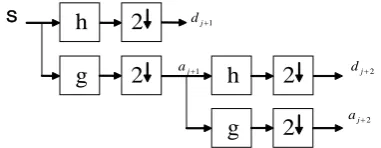
is function of the discrete wavelet, the transform can be represented, as a tree of low a high pass filter, with each step transforming the output of the low pass filter. Figure2 shows the wavelet decomposition tree, where the boxes represent linear convolution and circles represent down sampling by a factor of two (removal of every other sample). The original signal is successively decomposed into components of lower resolution, while the high frequency components are not analyzed any further. At each of the DWT algorithm, there are outputs: the scaling coefficients, j1

n

c and the wavelet coefficients, j1

n

d

.These coefficients are given respectively, by:

) ( ) 2 ( )

(

2

1 1

m c i m h m

c j

m

i

j





 _ _ (9)

) ( ) 2 ( )

(

2 1 1

m c i m g m

d j

m

i

j





 _ _ (10)

Here, g and h represent the low pass and high pass filters' transfer functions respectively. The output scaling coefficients are considered as the input samples to the next stage in the DWT algorithm [20-21]. The wavelet coefficients are described by:

) 1 2 ,..., 2 , 1 , 0

(  M 

M n

L n

d (11-1)

) 1 2 ,..., 2 , 1 , 0

( ₁

1 _ _

 

M M

n

L n

d (11-2)



) 1 2 ,..., 2 , 1 , 0 (

1 _ L_

n dn

(11-3)

L denotes the maximum number of scales that can be performed. It depends on the size of the data to be analyzed.

S dj1

aj1 dj2

aj2

2 h

g

h

g

2

Figure 2. The Structure of Discrete Wavelet Transform

The initial decomposition produces two sets of data: a set of approximation coefficients and a set of detail coefficients. The S in the first row represents the entire signal, with no decomposition. The first stage represents the first level of decomposition. There, node

1

 j

a shows the approximation coefficient and

1

 j

d states the detail coefficients. This stage

(3)

decomposition (M=5), the length of signal: 2048 samples (n=2048). All detail coefficients {d₅,d₄,d₃,d₂,d₁}

(1≤M≤5) and approximation coefficient a₅ (M=5) are assembled together in the coefficient vector (C):

] , , , , ,

[a5 d5 d4 d3 d2 d1

C

2.1. Orthogonal Wavelets (dbN, symN)

Let us recall that a multiresolution approximation is a nested sequence of linear space. The orthogonal complement

W

_j of

j

V

in

V

_j_₁can be thus defined:

j j

j V W

V 1   (12)

Then there is a function



such that the family

) 2

( 2 )

( /2

, t t n

j j

n

j  



 _

 , n in Z, is an orthonormal

basis of _W_j. The family n j,

 , j in Z and n in Z, is an orthonormal basis of L2 and:

k j k j j Z j

j W V W

V R

L2( )     (13)



is an orthogonal wavelet associated to the multi-resolution approximation [27]. A signal f in L2 can be decomposed as:



             Z

n k jn Z

n k n k n j n j n j Z n j n j t f t j t f t f , , , , , , , , ) ( , ) ( , ) ( , ) (       (14)

φ is an orthogonal scaling function of the multiresoution. One can verify the other resolutions are generated by a suitable dilatation of these bases of translated atoms. Since the resolutions are embedded, there is necessarily a sequence of real number h[n] such that:

) ( ] [ ) 2 ( 2 1 n t n h t n  



   

 (15)

In this study, we have examined the symN and dbN wavelet families that include: Sym8, Sym7, Sym5, db3 and db2.

2.2. Biorthogonal Wavelet (BiorN)

Leave Biorthogonal wavelets are defined similarly to orthogonal wavelets, except that the starting point is biorthogonal multi-resolution approximations. The following decompositions are performed:

  1  j j j ( j )

j V W withW V

V (16-1)

 

  

1 j  j j ( j)

j V W withW V

V (16-2)

Like in the orthogonal case, a signal in L can be written as:



                           Z n j k n k n k Z n n j n j n j Z n j n j Z

n k jn Z

n k n k n j n j Z n j n j n j t f t j t f t f t j t f t f , * , , * , , * , , , , , * , , * , , , * , ) ( , ) ( , ) ( , ) ( , ) ( , ) ( , ) (             (17)

In this paper, we have tested the Bior wavelet families that include: Bior4.4, Bior3.3, Bior3.1 and Bior2.2 as the biorthogonal wavelets.

3. THREE-LEVEL QUANTIZATION

In this section, the quantization of the coefficient vector (C) is described. Due to the quantization, perfect reconstruction is not possible, and reconstruction errors occur. The quantization is performed iteratively by a three-level quantizer. Given the input

vector C and the threshold



_i of the

i

th iteration, _i described by:          

,...( 1) . 2 1 ) 1 ),...( ] [ ( max . 2 1 1 i i k c i k i (18) N k1,2,...,



Where i

 is a threshold of the th

i iteration that is generated by the above equation for beginning of quantization. The coefficients of vector (C) are quantized by the quantizer that is defined by equation (19). The quantized coefficients

] [k d

n

 are described by:

                   



       else k d k c if k d k c if k

d i i

i n i i i n i i i , 0 ) ]. [ ] [ ( , 1 ) ]. [ ] [ ( , 1 ] [ 1 1 1 1 (19) N k1,2,..., 

In this stage, the input vector includes a set of approximation and detail coefficients that is created in the five levels of decomposition. Results of this step are the quantized coefficients vector (C) that is generated by the equation (19). The quantized coefficients that are named_d _[_k_]

n

 include

exclusively three symbols {-1, 0, 1}. Where _d__[_k_]₀

n

denotes

the insignificant coefficients that is not very important for reconstruction of the original signals and dn[k]1

the

significant ones that are very effective to decrease error rate. The wavelet coefficient cˆ[k] can be reconstructed by using the

quantized coefficients and the initial threshold₁:



     i n n k d k c n 1 1

1 [ ].2

] [

ˆ (20)

4. EZW AND HUFFMAN ENCODING

The EZW algorithm has two very interesting properties [22-23-24]. The first is that the EZW algorithm creates a connection between the wavelet coefficients from different sub-bands. This is the reason why several quantized coefficients from different sub-bands can be encoded using only one symbol .The second property is that the import coefficients are encoded using the successive approximated technique, which puts the most important parts of the coefficients at the beginning of a bit stream. Therefore, the encoder can easily stop encoding procedure at any desired target rate.

In this section, the encoding of the quantized coefficients is performed at each iteration level of the quantization procedure. The main goal of the encoding algorithm is to find a connection between the quantized coefficients

[.]

i

d

_ from different sub-band. Also we don’t need to calculate the threshold again by

] ) max( [log

2 C

thr equation because of the thresholding of the coefficient vector (C) in the previous section. Therefore in this stage, we only need to encode the results of the previous step to receive a better performance.

(4)

symbols {Z} describes those quantized coefficient, which are zero and do not belong to a zero-tree. The results of this stage are an encoded coefficients vector C with four symbols {P, N, T, Z}.

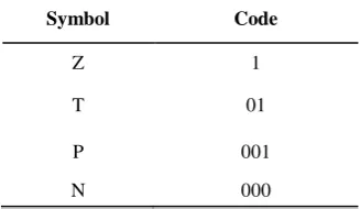
In the next stage, these coefficients with the Variable-Length Coding (Huffman Coding) are encoded. In the Huffman encoding, a code with shorter length is replaced by symbols that have a small number and a code with longer length is substituted by symbols that their number is very large. We have considered the number of each symbol and Z, T, P and N have been replaced by 1, 01, 001 and 000 codes, respectively. Table1 describes this procedure:

TABLE 1.ENCODING SYMBOLS IN THE HUFFMAN ALGORITHM

Symbol Code

Z 1

T 01

P 001

N 000

5. SIMULATION RESULTS

In this section, we have compared the result of several experiments of our method with other ECG coders. The proposed algorithm was tested and evaluated using actual data from MIT-BIH arrhythmia database. These ECG databases were sampled at 360 Hz with the Resolution of 11 bits/sample. We have used Daubechies (db3, db2), Symlet (sym8, sym7, sym5) and Biorthogonal wavelets (Bior2.2, Bior3.1, Bior3.3, Bior2.6, Bior4.4) with five levels of decomposition. The following results have been obtained using the records number: 101, 103, 105, 115, 117, 118, 119, 201, 205, 213 and 219. To gain an optimum performance, 2048 samples and 3 types of wavelet with 5-level decompression have been used for compression of ECG signals. In order to validate the proposed compression algorithm and to compare it with other methods, 11 records consisting of the 2048 samples from the MIT-BIH Arrhythmia database have been used. The ECG signals were digitized through sampling at 360 (samples/s), quantized and encoded with 11 bits.

We have compared the performance of our encoder with some kinds of encoders in the literature, wavelet-based coders and direct ECG signal coders. The PRD and CR results in a similar record have been compared. Now, the effects of the iterations of the three-level quantization on the PRD, CR have been evaluated.

TABLE 2.A COMPRESSION OF DIFFERENT ENCODING ALGORITHM FOR RECORD 117

Algorithms PRD (%) CR (%)

JPEG2000 [25] 1.03 10:1

Sec & SPIHT [26] 1.01 8:1

SPIHT & VQ [27] 1.45 8:1

SPIHT [28] 1.8 8:1

Hilton [35] 2.6 8:1

WT & Huffman [11] 3.2 9.4:1

Djohn [36] 3.9 8:1

Wavelet Neural Network [33] 2.74 7.6:1

Jianhua Chen [32] 1.08 12:1

the block-based discrete

cosine transform (DCT )[34] 1.18 9.56:1

RLE [29] 2.915 5.8:1

ASCII [30] 7.89 15.72:1

Benzid [9] 3.51 12.6:1

Dc Equalization and

Complexity Sorting [31] 1.118 13.75:1

Proposed Technique 0.97 13.92:1

Table 2 shows the performance of the different algorithms in comparison with our simulated results. According to the table, there are some ECG compression methods in the literature, The Wavelet Neural Network, RLE, Benzid, Jianhua Chen, Hilton, SPIHT, SPIHT&VQ, Sec&SPIHT and WT&Huffman methods have presented a wavelet and wavelet packet-based EZW encoder [7]. They have reported respectively the PRD values of 2.74%, 2.915%, 3.51, 1.08, 2.6%, 1.8%, 1.45%, 1.01% and 3.2 with CR lower than 13. Also by comparison with other coders, the PRD ranges of 1.18%, 1.03% and 3.9% in Table 2 are significantly higher (inferior) compared to our results and also, their CR values of 9.56%, 10% and 8% are noticeably lower (inferior) in comparison with our presented results. In ASCII [36] a combination of CR and PRD that has been received is so bad. In table 2, the best combination of CR and PRD values of the coder compared here which is considerably better than others is 13.75:1% and 1.118% for the Dc Equalization and Complexity Sorting method [38]. The proposed compression algorithm in this paper obtain an excellent performance (PRD=0.97% and CR=13.92:1%) that is extremely better than other coders.

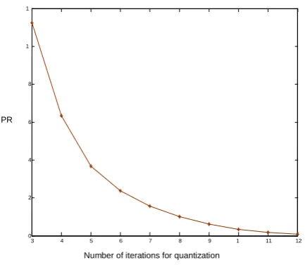
Figure 3 shows the effects of the iterations of quantization on PRD. According to the Figure, as the numbers of iterations increase, the values of PRD can be improve more and in low number of iterations, the PRD values increase sharply and it would be worse than. Fig. 4 shows the effects of the iterations of quantization on CR. It can be found from the Figure 4 that the values of CR would be increased when the numbers of iteration become lower. In other words, by decreasing the numbers of iteration, the values of CR can be better and by increasing iterations, the CR values would be worse.

[image:4.595.88.252.221.316.2] [image:4.595.67.279.617.764.2]

(5)

[image:5.595.62.279.66.473.2]

Figure 3. The effects of the iterations of quantization on PRD

Figure 4. The effects of the iterations of quantization on CR

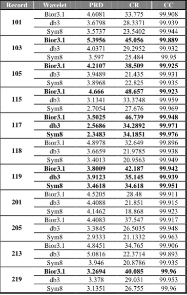
[image:5.595.63.280.71.259.2]

Table 3 shows the achieved results for compression of the 9th iteration. The highest compression ratio (CR=15.3670%) was achieved using Bior3.1for record number 115. The lowest percent root-mean-square different (PRD=0.61511%) was achieved using sym8 for record no. 117. The correlation coefficients (CC) for all the records in 9th iteration are very excellent (CC>99.99%). But it is noted that the performance of the compression algorithm is dependent on CR, PRD and CR together. Because of it, the highest compression performance was achieved for record 219 using Bior3.1 with a CR of 13.9839%, a PRD value of 0.71706% and CC=99.998%. The fonts of the other better performances are boldface in Table 3. (e.g. For record 219 using Sym8 wavelet, CR=11.92%, PRD=0.75792%, CC=99.997%. For record 119 using Bior3.1 wavelet, CR=13.2362%, PRD=0.86724%, CC=99.996%. For record 117 using Sym8, CR=9.3014%, PRD=0.61511%, CC=99.998%)

Table 3. Results of the proposed algorithm in 9th_iteration

of quantization using bior, db and sym wavelets for 11 records with n=2048 samples.

CC CR

PRD Wavelet

Record

999999 9.0802

1.0904 Bior3.1

101 db3 6999999 0979.6 999999

999999 092569

69999.0 Sym8

99.992 13.579

1.2863 Bior3.1

103 db3 699955 995977 999992

999990 999629

6995955 Sym8

99.995 9.3361

0.9803 Bior3.1

105 db3 6977025 099700 999999

999999 097909

697797 Sym8

999999 15.3670 1.0748

Bior3.1

115 db3 6999929 9999.2 999999

999997 79972.

69009.7 Sym8

99.997 11.976

0.82503 Bior3.1

117 db3 6902..9 799027 999997

999999 9903.9

395.9.. Sym8

99.995 11.5174 0.99121

Bior3.1

118 db3 69970.7 792697 999999

999999 999022

6999097 Sym8

99.996 13.2362 0.86724

Bior3.1

119 db3 6992.70 .59772 999990

999999 .69959

3999969 Sym8

99.995 8.7419

1.0062 Bior3.1

201 db3 69796 097929 999990

999990 095920

697699 Sym8

99.995 12.2835 1.0027

Bior3.1

205 db3 699.79 997697 999999

999999 999290

690929 Sym8

99.996 14.0888 0.97583

Bior3.1

213 db3 .9690 99797 999992

999999 99.970

697799 Sym8

99.998 13.9839 0.71706

Bior3.1

219 db3 6999697 .6929. 999999

999999 ..996

3999996 Sym8

It can be found from comparison of Table 3 and Table 4 that the values of CR and PRD decreased and the value of CC increased, when the numbers of iteration become higher. In other words, in the higher numbers of iteration, the PRD and CC performances become better values and the value of CR would be worse. Table 4 shows the achieved results for compression of the 8th iteration. The highest compression ratio (CR=5790079%) was achieved using Bior3.1for record no. 115.

The lowest percent root-mean-square different

(PRD=0.99699%) was achieved using sym8 for record no. 117. The correlation coefficients (CC) for most of the records in 9th iteration are very excellent (CC>99.99%). But generally, the performance of the compression algorithm is dependent on CR, PRD and CR together. The highest compression performance was achieved for record 219 using Bior3.1 wavelet with CR=18.3154%, PRD=1.1508% and CC=99.994%. And the other better performances are highlighted with boldface in Table 4. As seen from Table 4, some better performances are: record 219 using Bior3.1 wavelet with values of CR=11.18.3154%, PRD=1.508% and CC=99.997%. Record 119 using db3 wavelet has the values of CR=21.293%, PRD=1.5276% and CC=99.989%.

3 4 5 6 7 8 9 10 11 1

0 10 20 30 40 50 60 70

C

Number of iteration for quantization

3 4 5 6 7 8 9 1 11 12

0 2 4 6 8 1 1

[image:5.595.331.525.100.406.2] [image:5.595.66.276.273.471.2]

(6)

[image:6.595.76.270.101.407.2]

Table 4. Results of the proposed algorithm in 8th_{iteration of}

quantization using bior, db and sym wavelets for 11 records with n=2048 samples

CC CR PRD Wavelet Record 99.984 12.7349 1.8531 Bior3.1

101 db3 .99999 797979 999979

99999 799597 .99577 Sym8 99.981 23.1056 2.0404 Bior3.1

103 db3 .99299 .6929.9 999972

999977 .69762 .92999 Sym8 99.987 12.9994 1.6608 Bior3.1

105 db3 .92929 79077 999977

999979 996.79 .99979 Sym8 99.986 23.6639 1.7895 Bior3.1

115 db3 .97695 .595907 999995

999999 .796556 .96750 Sym8 99.992 15.8648 1.3217 Bior3.1

117 db3 .969.9 .79999 999999

999999 .099609 3999399 Sym8 99.986 15.7980 1.7186 Bior3.1

118 db3 .97702 ..95729 99999.

999997 ..90790 .95795 Sym8 99.991 18.4052 1.4276 Bior3.1

119 db3 .99695 6.9690 999999 999996 .99939 .909.9 Sym8 99.987 10.3959 1.668 Bior3.1

201 db3 .90255 99722 999970

999979 9900 .92600 Sym8 99.988 14.5342 1.6166 Bior3.1

205 db3 .95965 ..9677 99999.

999999 .5969. .9.629 Sym8 99.987 18.0224 1.7402 Bior3.1

213 db3 .97520 .590996 999972

99999. .595070 .99662 Sym8 99.994 18.3154 1.1508 Bior3.1

219 db3 .95999 .797.5 999997

999999 .79092

[image:6.595.75.270.102.406.2]

.9.769 Sym8

Table 5. Results of the proposed algorithm in 7th iteration of

quantization using bior, db and sym wavelets for 11 records with n=2048 samples.

CC CR PRD Wavelet Record 99990 569295 599777 Bior3.1

101 db3 599267 .997999 999995

999997 .99.290 599662 Sym8 999999 0.9939 09.959 Bior3.1

103 db3 597655 5799.79 999909

999990 609059 6995 Sym8 999902 5796.. 599279 Bior3.1

105 db3 590700 .29.0 999909

999995 .99629 599057 Sym8 999959 099939 699659 Bior3.1

115 db3 596299 5697569 99997.

999999 .993559 .95599 Sym8 999999 699936 69.955 Bior3.1

117 db3 .95909 6399933 999999 99999 6399.90 .99.69 Sym8 999905 569592 597955 Bior3.1

118 db3 595769 .299690 999999

99997 .099999 59..0 Sym8 999999 599607 597657 Bior3.1

119 db3 690900 699965 999995 99999. 699090 69.069 Sym8 999905 .996.2 597970 Bior3.1

201 db3 597952 ..9095 999905

999909 .69957 592907 Sym8 999909 579792 599.7 Bior3.1

205 db3 596929 .9999.6 99997

999979 .79625. .90929 Sym8 999907 5996079 599270 Bior3.1

213 db3 796799 .990.77 999906

999990 .099.59 597099 Sym8 999999 699399 .99959 Bior3.1

219 db3 596907 569299 99997.

999990 609690

.995.9 Sym8

Table 5 shows the achieved results for compression of the 7th iteration. The best compression ratio (CR=779967%) was achieved using Bior3.1for record no. 115. The lowest percent root-mean-square different (PRD=.92.57%) was achieved using sym8 for record no. 117. The highest correlation coefficient (CC) was obtained using sym8 wavelet for record number 117. But the performance of the compression is dependent on CR, PRD and CR. With this explanation, the highest compression performance was achieved for record 219 using Bior3.1 wavelet with CR=27.077%, PRD=1.8968% and CC=99.985%. It can be found from the table, some better performances are: record 115 using Bior3.1 wavelet with CR=38.708%, PRD=2.9269%, CC=99.965%. Record 117 using

sym8 wavelet with CR=5692.97%, PRD=1.5128%,

CC=99.99%. Record 219 using Bior3.1 wavelet with the values of CR=27.077%, PRD=1.8968%, CC=99.985%.

[image:6.595.69.269.443.749.2]

Table 6 and 7 show the simulation results of the proposed algorithm for 6th and 5th iterations. In these iterations, the values of CR and PRD are higher and the value of CC is lower. On the other hands, in the 6th and 5th numbers of iteration, the CR performance become better values and the values of PRD and CC would be worse. For iterations lower than 5, the compression ratio (CR) was achieved extremely high (the high CR is our favorite) but the percent root-mean-square different (PRD) that is a very important factor, was inferior (the value of PRD become high too whereas the low PRD is our preferable). And also for iterations higher than 9, the percent root-mean-square different (PRD) was obtained extremely low (the lower PRD is our admirable) but in these iterations, the compression ratio (CR) was achieved lower whereas the low CR is inferior. Because of it, we show the simulation results from 5th to 9th iteration.

Table 6. Results of the proposed algorithm in 6th iteration of

CC CR PRD Wavelet Record 999967 779992 99067. Bior3.1

101 db3 790997 579779. 999979

999999 5792965 792979 Sym8 999999 999395 990995 Bior3.1

103 db3 99679. 5995925 999975

99992 529979 79299 Sym8 999969 099939 996.39 Bior3.1

105 db3 799979 5.9972 99997.

999972 559752 797907 Sym8 999960 999599 99555 Bior3.1

115 db3 79.79. 7797997 999929

999909 599090 599629 Sym8 999999 959909 099369 Bior3.1

117 db3 699595 0996996 99999. 999995 099.99. 690990 Sym8 999790 759099 997997 Bior3.1

118 db3 790029 5.99972 999977

999999 5699207 7996.7 Sym8 999996 969.99 099339 Bior3.1

119 db3 099.60 099.99 999909 99999. 0995.9 0995.9 Sym8 9999.. 57997 992562 Bior3.1

201 db3 999677 5.972. 9999.2

999957 .79707 99.905 Sym8 9999.9 799299 999677 Bior3.1

205 db3 797792 5092672 999997

999907 5.9.775 599777 Sym8 999960 799902 99792. Bior3.1

213 db3 2967.0 55979.9 999797

999972 5697970 79990 Sym8 99995 939399 096599 Bior3.1

219 db3 79797 59967. 999927

99990 509922

[image:6.595.332.524.444.747.2]

(7)

[image:7.595.75.270.103.407.2]

Table 7. Results of the proposed algorithm in 5th_{iteration of}

CC CR

PRD Wavelet

Record

999765 979999

99.929 Bior3.1

101 db3 2997.2 779299 999799

999777 59979.0

299799 Sym8

999969 259777

99567. Bior3.1

103 db3 090625 759.759 999779

999709 759065

096799 Sym8

99979. 929990

09977 Bior3.1

105 db3 099967 70992 999759

999797 779999

095.0 Sym8

999977 29999.

796909 Bior3.1

115 db3 999609 969.990 999939

999959 79995

997202 Sym8

999936 909339

990990 Bior3.1

117 db3 99.999 99999.9 99990. 99999. 969.990

099359 Sym8

999929 269797

999967 Bior3.1

118 db3 297029 959260 999799

999707 769979

29095 Sym8

999999 909099

590696 Bior3.1

119 db3 099.77 999975 9997.9

999799 779999

299569 Sym8

999769 959260

996595 Bior3.1

201 db3 092599 7.9267 999759

99977 59959.

097769 Sym8

999752 979707

99.962 Bior3.1

205 db3 29.66. 7799977 999795

999967 7697067

99979. Sym8

99997. 9597929

797792 Bior3.1

213 db3 7996.6 7.96767 999099

9997.2 509777.

097979 Sym8

999999 969999

999639 Bior3.1

219 db3 290905 79970 999799

999770 7.9579

[image:7.595.305.550.125.369.2]

292027 Sym8

Table 8. A comparison of the average of PRD and CR based on the different wavelets and iterations of quantization

Iteration Wavelet PRD (%) CR (%)

9th

Bior3.1 0.983370 12.108180

db3 0.840505 8.306609

Sym8 0.768781 8.671600

8th

Bior3.1 1.635209 16.712700

db3 1.464164 11.932481

Sym8 1.305449 11.903890

7th

Bior3.1 2.693036 25.853581

db3 2.387445 18.603245

Sym8 2.122491 18.025000

6th

Bior3.1 4.374991 38.949909

db3 3.745418 27.601063

Sym8 3.376809 25.174490

5th

Bior3.1 7.136664 50.049263

db3 6.038873 37.717381

Sym8 5.561527 32.959663

Table 8 shows the average values of the performance accuracy at 9th, 8th, 7th, 6th and 5th iterations for all the eleven records. Because the correlation coefficients (CC) for all the proposed records in all iterations are very excellent (CC>99%), we have only calculated the average values of the PRD and CR for Bior3.1, db3 and Sym8 wavelets. As expected, the PRD is generally low and the compression ratio (CR) is achieved low at higher iterations and for lower iterations, the PRD and CR values are achieved higher. It can be seen from theTable8, The best compression ratio (CR=50.17449%) was obtained using Bior3.1 and the lowest percent root-mean-square different was achieved (PRD=6990797.%) using sym8 wavelet for all the considered records. But as we mentioned before, the best

performance depends on both CR and PRD. Therefore according to the values, the Bior3.1 and sym8 are achieved the best performances. The lower PRDs are achieved by sym8 wavelet and the higher CRs are achieved by Bior3.1 for all the considered iterations.

(a)

(b)

(c)

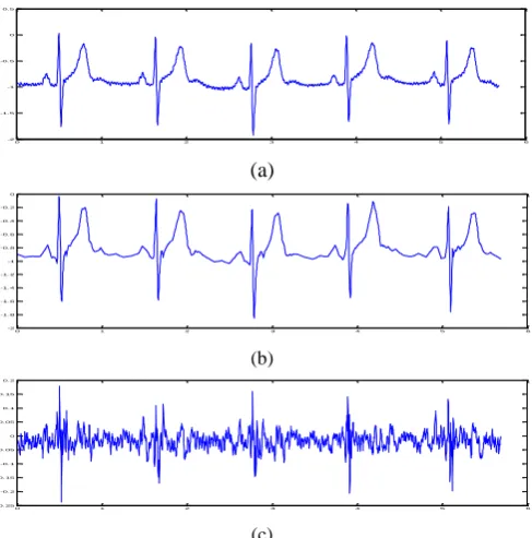
Figure 5. (a) Original signal, (b) Reconstructed signal, (c) Error signal.

ECG compression using Bior2.2 wavelet and 2048 samples of signal and 5th iteration of quantization for record no. 117 from MIT-BIH database (CR=59.9149, PRD=4.2883, CC=99.928)

(a)

(b)

(c)

ECG compression using db3 wavelet and 2048 samples of signal and 5th iteration of quantization for record no. 117 from MIT-BIH database (CR=45.8819, PRD=4.1879, CC=99.931)

0 1 2 3 4 5 6

-2 -1.5 -1 -0.5 0 0.5

0 1 2 3 4 5 6

-2 -1.8 -1.6 -1.4 -1.2 -1 -0.8 -0.6 -0.4 -0.2 0

0 1 2 3 4 5 6

-0.25 -0.2 -0.15 -0.1 -0.05 0 0.05 0.1 0.15 0.2 0.25

0 1 2 3 4 5 6

-2 -1.5 -1 -0.5 0 0.5

0 1 2 3 4 5 6

-2 -1.8 -1.6 -1.4 -1.2 -1 -0.8 -0.6 -0.4 -0.2 0

0 1 2 3 4 5 6

[image:7.595.305.549.434.681.2] [image:7.595.51.291.434.624.2]

(8)

(a)

(b)

(c)

ECG compression using Bior3.1 wavelet and 2048 samples of signal and 8th_{iteration of quantization for record no. 115 from}

MIT-BIH database (CR=23.6639, PRD=1.7895, CC=99.986)

(a)

(b)

(c)

(a)

(b)

(c)

ECG compression using Bior4.4 wavelet and 2048 samples of signal and 8th iteration of quantization for record no. 119 from

(a)

(b)

(c)

ECG compression using Sym7 wavelet and 2048 samples of signal and 9th iteration of quantization for record no. 119 from MIT-BIH database (CR=12.364, PRD=0.82527, CC=99.997)

0 1 2 3 4 5 6

-1.5 -1 -0.5 0 0.5 1 1.5 2

0 1 2 3 4 5 6

-1.5 -1 -0.5 0 0.5 1 1.5 2

0 1 2 3 4 5 6

-0.2 -0.15 -0.1 -0.05 0 0.05 0.1 0.15

0 1 2 3 4 5 6

-1.5 -1 -0.5 0 0.5 1 1.5 2

0 1 2 3 4 5 6

-1.5 -1 -0.5 0 0.5 1 1.5 2

0 1 2 3 4 5 6

-0.03 -0.02 -0.01 0 0.01 0.02 0.03

0 1 2 3 4 5 6

-2.5 -2 -1.5 -1 -0.5 0 0.5 1 1.5 2

0 1 2 3 4 5 6

-2.5 -2 -1.5 -1 -0.5 0 0.5 1 1.5 2

0 1 2 3 4 5 6

-0.08 -0.06 -0.04 -0.02 0 0.02 0.04 0.06

0 1 2 3 4 5 6

-2.5 -2 -1.5 -1 -0.5 0 0.5 1 1.5 2

0 1 2 3 4 5 6

-2.5 -2 -1.5 -1 -0.5 0 0.5 1 1.5 2

0 1 2 3 4 5 6

[image:8.595.44.549.74.322.2] [image:8.595.45.542.393.635.2]

(9)

(a)

(b)

(c)

ECG compression using sym8 wavelet and 2048 samples of signal and 8th iteration of quantization for record no. 119 from MIT-BIH database (CR=13.923, PRD=0.97044, CC=99.995)

(a)

(b)

(c)

ECG compression using db2 wavelet and 2048 samples of signal and 8th_{iteration of quantization for record no. 117 from}

(a)

(b)

(c)

ECG compression using sym5 wavelet and 2048 samples of signal and 8th iteration of quantization for record no. 117 from MIT-BIH database (CR=13.346, PRD=1.0594, CC=99.998)

(a)

(b)

(c)

Figure14. (a) Original signal, (b) Reconstructed signal, (c) Error signal.

0 1 2 3 4 5 6

-2 -1.5 -1 -0.5 0 0.5

0 1 2 3 4 5 6

-2 -1.5 -1 -0.5 0 0.5

0 1 2 3 4 5 6

-0.03 -0.02 -0.01 0 0.01 0.02 0.03 0.04

0 1 2 3 4 5 6

-2 -1.5 -1 -0.5 0 0.5

0 1 2 3 4 5 6

-2 -1.5 -1 -0.5 0 0.5

0 1 2 3 4 5 6

-0.04 -0.03 -0.02 -0.01 0 0.01 0.02 0.03 0.04

0 1 2 3 4 5 6

-2 -1.5 -1 -0.5 0 0.5

0 1 2 3 4 5 6

-2 -1.5 -1 -0.5 0 0.5

0 1 2 3 4 5 6

-0.04 -0.03 -0.02 -0.01 0 0.01 0.02 0.03

0 1 2 3 4 5 6

-2.5 -2 -1.5 -1 -0.5 0 0.5 1 1.5 2

0 1 2 3 4 5 6

-2.5 -2 -1.5 -1 -0.5 0 0.5 1 1.5 2

0 1 2 3 4 5 6

[image:9.595.47.549.74.331.2]

(10)

6. CONCLUSION

The proposed algorithm for compression of ECG signals using wavelet transforms and EZW& Huffman encoding based on the three-level quantization is described in this Paper. The algorithm is examined for compression of 11 records of ECG signal from the MIT-BIH database. The experimental results indicate that the presented wavelets in this coder have high performance. The some of biorthogonal wavelets have a performance better than the orthogonal wavelets. In this paper, combination of three-level quantization and EZW together for thresholding and encoding has been used. After selecting threshold, the three-level quantization has been continued from 1th level to 12th level of iteration. In low iterations, the values of CR and PRD are higher and the value of CC is lower. On the other hands, in the lower numbers of iteration, the compression ratio (CR) is achieved extremely high (CR become better values) but the percent root-mean-square different (PRD) that is a very important factor, is inferior (the value of PRD become high too whereas the low PRD is our favorite). And also for high iterations, the PRD is obtained extremely low (the lower PRD is our admirable) but in these iterations, the CR values are achieved lower whereas the low CR is inferior. Consequently, it seems reasonable to conclude that the best simulation results are achieved for 5th to 9th iterations. The three kinds of wavelet were tested to gain the acceptable results named: db, bior and sym.

The different results have gained for each wavelet and record number. Among all wavelets, in higher iterations, sym8 and some of biorthogonal wavelets (bior2.2, bior3.3, bior3.1 and bior4.4) achieved better results. Also, we have concluded that if high compression rates need, we should continue iterations of quantization for lower than 4th_{level. Consequently, if we want}

to decrease the PRD value, the iterations of the three-level quantizer can be continued to high levels. Generally, for values of CR>50 and 3.5<PRD, the three-level quantization should be continued to 4th or 5th level of iteration. If a ratio around 24<CR<50 and 1.5<PRD<3.5 is our favorite, we should repeat the three-level quantization to 6th or 7th iteration. For 6<CR<24 and 0.6<PRD<1.7, it should be quantized to 8th or 9th iteration. And for about 0<CR<10 and 0<PRD<0.6, the three-level quantization can be repeated to 10th or more. The number of iteration depends on our particular application in which value of CR and PRD should be used to gain our favorite results.

7. REFERENCES

[1] J. R. Cox, F. M. Nolle, H.A. Fozzard, and G. C. Oliver.

''AZTEC, a preprocessing program for real time ECG rhythm analysis '' IEEE Trans. Biomed. Eng. Vol, BME-15, pp. 128-129, 1968.

[2] J. P. Aberstein and W. J. Tompkins,"A new data reduction algorithm for real time ECG analysis" IEEE Trans.

Biomed. Eng. Vol. BME-29, pp. 43-48, 1982.

[3] Z. Lu, D. Y. Kim, and W. A. Pearlman, “Wavelet

compression of ECG signals by the set partitioning in hierarchical trees algorithm,” IEEE Trans. Biomed. Eng., vol. 47, pp. 849-856, July 2000.

[4] S. G. Miaou, H. L. Yen and C. L. Lin, “Wavelet-based

ECG compression using dynamic vector quantization with tree codevectors in single codebook,” IEEE Trans. Biomed. Eng., vol. 49, pp. 671-680, July 2002.

[5] S. G. Miaou and S. N. Chao, “Wavelet-based lossy-to-lossless ECG compression in a unified vector quantization framework,” IEEE Trans. Biomed. Eng., vol. 52, pp. 539-543, March 2005.

[6] A. Al-Shroufa, M. Abo-Zahhad and Sabah M. Ahmedc, “A novel compression algorithm for electrocardiogram signals based on the linear prediction of the wavelet coefficients,” Digital Signal Processing, Elsevier, vol. 13, pp. 604-622, October 2003.

[7] A. Alshamali and A.S. Al-Fahoum, “Comments on "An efficient coding algorithm for the compression of ECG signals using the wavelet transform,” IEEE Trans. Biomed. Eng., vol. 50, pp. 1034-1037, August 2003.

[8] J. Chen, J. Ma, Y. Zhang and X. Shi, “ECG compression

based on wavelet transform and Golomb coding,” Electron.Lett., vol. 42, no. 6, pp. 322-324, March 2006

[9] R. Benzid, F. Marir and N. E. Bouguechal, “Electrocardiogram Compression Method Based on the Adaptive Wavelet Coefficients Quantization Combined to a Modified Two-Role Encoder,” IEEE Signal Pro, Lett, vol. 14, pp. 373-376, June 2007.

[10] P. S. Hamilton, “Adaptive compression of the ambulatory electrocardiogram,” Biomed. Inst. Technol., vol. 27, no. 1, pp. 56-63, Jan. 1993.

[11] A. Al-shrouf, M. Abo-Zahhad, S. M. Ahmed. '' A novel compression algorithm for electrocardiogram signal based on the linear prediction of the wavelet coefficients '' Digital

Signal Processing, Vol.13, 2003, pp. 604-622.

[12] M. Blanco-Velasco, F. Cruz-Roldan, J. I. Godino-Llorente and K. E. Barner, “Wavelet Packets Feasibility Study for the Design of an ECG Compressor,” IEEE Trans. Biomed. Eng., vol. 54, pp. 766-769, April 2007.

[13] J. M. Shapiro,"Embedded Image Coding Using Zero-Trees of wavelet Coefficients", IEEE Trans. On Signal

Processing, vol. 41. NO. 12. pp. 3445-3462, 1993.

[14] Said A, Pearlman WA. A new, fast, and efficient image codec based on set partitioning in hierarchical tree. IEEE Trans. CSVT 1996;6(3):243-50.

[15] Gersho A, Gray RM. Vector Quantization and Signal Compression. New York: Kluwer Academic Press, 1992.

[16] Sang Joon Lee and Myoung ho Lee 30th Annual International IEEE Conference Vancouver, British Columbia, Canada , August 20-24, 2008

[17] H. L. Chan, Y. C. Siao, S. W. Chen and S. F. Yu, “Wavelet-based ECG compression by bit-field preserving and running length encoding”, Computer Methods and Prog. in Biomedicine, vol.90, pp.1-8, 2008.

[18] C. M. Fira and L. Goras, “An ECG signals Compression

Method and its Validation using NNs”, IEEE Trans Biomed. Eng, vol. 55, No. 4, pp. 1319-1326, 2008.

[19] H. Kim, R. F. Yazicioglu, P. Mercen, C. V. Hoog and H. J. Yoo, “ECG signal compression and classification with Quad Level Vector for ECG Holter system”, IEEE Trans. Inf. Tech. in Biomed, vol.14, No.1, pp. 93100, 2010.

[20] C. S. Burrus. R. A. Gopinath. H. Guo, introduction to

Wavelets and Wavelet Transforms, Prentice-Hall, 1997.

[21] S. G. Mallat,“A Theory of Multiresolution signal decompression; The Wavelet Representation”, IEEE Trans.

Image Processing, vol. 1, no. 2, pp. 205-220, April 1992.

[22] J. M. Shapiro,"Embedded Image Coding Using Zero-Trees of wavelet Coefficients", IEEE Trans. On Signal

(11)

International Journal of Computer Applications (0975 – 8887) Volume 59– No.1, December 2012 [23] P. Wellig, Z. Cheng, M. Semling, and G. S. Moschytz, "

Electromyogram Data Compression Using Signal-Tree and Modified Zero-Tree Wavelet Encoding ", Proceeding of the 20th Annual International Conference of the IEEE Engineering in medicine and biology society, Vol. 20, No.

3, pp. 1303-1306, 1998.

[24] L. M. Ang, H. N. Cheung, and K. Eshraghian, "EZW Algorithm Using Depth-First Representation of the Wavelet Zero-Tree" , 5th International Symposium on

Signal Processing and its Applications, pp. 75-78, 1999.

[25] Ali Bilgin, Michael W. Marcellin, Maria I. Altbach,"

Compression of Electrocardiogram Signals Using JPEG2000 " , IEEE Transactions on Consumer Electronics, Vol. 49, No. 4, November, 2003, pp. 833-840.

[26] I. M. Rezazadeh. M. H.Moradi, A.M. Nasrabadi, "Implementing of SPIHT and subband Energy Compression (SEC) Method on Two-Dimensional ECG Compression: A Novel Approach”. Engineering in medicine and biology, 27th annual conference, IEEE, China, 2005.

[27] S. M. E Sahraeian and E. Fatemizadeh. "Wavelet-Based 2-D ECG 2-Data Compression Method Using SPIHT and VQ Coding ". IEEE Int. Conf on " Computer as a tool" . EUOROCON 2007.

[28] Z. Lu, D. Y. Kim, and W. A. Pearlman, "Wavelet Compression of ECG signal by the Set Partitioning in Hierarchical Trees (SPIHT) algorithm" IEEE Transactions on Biomedical Engineering, Vol. 47, July 2000 , pp. 849-856.

[29] Ranjeet Kumar, A. Kumar, Rajesh K. Pandey “Beta wavelet based ECG signal compression using lossless encoding with modiﬁed thresholding” Computers and Electrical Engineering (Elsevier 2012)

[30] S.K. Mukhopadhyay, S. Mitra, , M. Mitra ”An ECG signal compression technique using ASCII character encoding”

Measurement (Elsevier) 45, 2012, pp. 1651–1660

[31] Eddie B . L . Filho, Nuno M. M. Rodrigues, Eduardo A. B . da Silva, S ´ ergio M . M . d e Faria , Vitor M . M . da S ilva, and M urilo B. de Carvalh,”ECG Signal Compression Based on Dc Equalization and Complexity Sorting” IEEE

TRANSAC TIONS ON BIOMEDICAL ENGINEERING, VOL. 55, NO. 7, JULY 2008

[32] Jianhua Chen, Fuyan Wang, Yufeng Zhang, Xinling Shi “ECG compression using uniform scalar dead-zone quantization and conditional entropy coding” Medical

Engineering & Physics (Elsevier), 30-2008, pp. 523–530

[33] R. Benzid, A. Messaoudi, A. Boussaad “Constrained ECG compression algorithm using the block-based discrete cosine transform” Digital Signal Processing 18 (2008) 56–

64

[34] Jin Wang, Xiaomei Lin and Kebing Wu “ECG Data Compression Research Based on Wavelet Neural Network” 2010 International Conference on Computer, Mechatronics, Control and Electronic Engineering (CMCE)

[35] Hilton ML. Wavelet and Wavelet Packet compression of electrocardiograms. IEEE Transactions on Biomedical Engineering 1997;44(5):394-402.