Munich Personal RePEc Archive
Exchange-rate policy and the zero bound
on nominal interest rates
Coenen, Gunter and Wieland, Volker
European Central Bank
January 2004
Online at
https://mpra.ub.uni-muenchen.de/76687/
PRELIMINARY DRAFT
Exchange-Rate Policy and the Zero Bound
on Nominal Interest Rates
∗
,†G¨unter Coenen European Central Bank
Volker Wieland
Goethe University of Frankfurt
First version: January 2004 This version: March 2004
Abstract
In this paper, we study the effectiveness of monetary policy in a severe recession and defla-tion when nominal interest rates are bounded at zero. We compare two alternative proposals for ameliorating the effect of the zero bound: an exchange-rate peg and price-level target-ing. We conduct this quantitative comparison in an empirical macroeconometric model of Japan, the United States and the euro area. Furthermore, we use a stylized micro-founded two-country model to check our qualitative findings. We find that both proposals succeed in generating inflationary expectations and work almost equally well under full credibility of monetary policy. However, price-level targeting may be less effective under imperfect credibility, because the announced price-level target path is not directly observable.
JEL Classification System: E31, E52, E58, E61
Keywords: monetary policy rules, zero-interest-rate bound, liquidity trap, rational expec-tations, nominal rigidities, exchange rates, monetary transmission.
∗Correspondence: Coenen: Directorate General Research, European Central Bank, Kaiserstrasse 29,
D-60311 Frankfurt am Main, Germany, phone: +49 69 1344-7887, e-mail: [email protected], homepage: http://www.guentercoenen.com; Wieland: Professur f¨ur Geldtheorie und -politik, Johann-Wolfgang-Goethe Universit¨at, Mertonstrasse 17, D-60325 Frankfurt am Main, Germany, phone: +49 69 798-25288, e-mail: [email protected], homepage: http://www.volkerwieland.com.
†This paper was prepared for the Annual Meeting of the American Econonomic Association in San Diego,
1
Introduction
Due to the recent experience in Japan the threat of deflation and a liquidity trap has taken
center stage in the debate on the proper formulation of monetary policy. Deflationary
episodes present a particular problem for monetary policy because the effectiveness of its
main instrument, the short-term nominal interest rate, may be limited by the zero lower
bound.1 With interest rates near zero, the central bank will not be able to offset recessionary
shocks by lowering nominal and thereby real interest rates. Furthermore, deflationary shocks
may raise real interest rates and worsen such a recession.
Researchers, practitioners and policymakers alike have made proposals for avoiding and
if necessary escaping deflation.2 In this paper, we focus on two proposals that have domi-nated the debate most recently: an exchange-rate peg and price-level targeting. Svensson
(2001, 2002, 2003), in particular, has emphasized that the central bank may create
expecta-tions of inflation by devaluing and pegging the exchange rate for some time.3 Alternatively, the central bank can try to manage expectations regarding future interest-rate policy by
announcing a target path for the price level and thus induce inflationary expectations.
The latter proposal goes back to Wolman (1998) but has been pushed most recently by
Eggertsson and Woodford (2003).
Our objective is to compare the effectiveness of an exchange-rate peg and price-level
targeting in stimulating the Japanese economy in a severe recession and deflation scenario
when nominal interest rates are bounded at zero. We conduct a quantitative evaluation in
the estimated macroeconomic model with rational expectations and nominal rigidities of
Coenen and Wieland (2002) that covers the three largest economies, the United States, the
1Nominal interest rates on deposits cannot fall substantially below zero, as long as interest-free currency
constitutes an alternative store of value (McCallum (2000)).
2See for example, Krugman (1998), Wolman (1998, 2003), Meltzer (1998, 1999), Posen (1998), Orphanides
and Wieland (1998, 2000), Buiter and Panigirtzoglou (1999), Buiter (2001), Goodfriend (2000), Clouse et al. (2000), Johnson et al. (1999), Benhabib, Schmitt-Groh´e and Uribe (2002), Svensson (2001, 2002, 2003), Bernanke (2002), Eggertsson (2003), Eggertsson and Woodford (2003), McCallum (2002), Coenen and Wieland (2003) and Adam and Billi (2003).
3Related proposals for depreciating the exchange rate have been made by Orphanides and Wieland (2000)
euro area and Japan. We recognize the zero-interest-rate bound explicitly in the analysis and
use numerical methods for solving nonlinear rational expectations models.4 Since this model
is not fully developed from microeconomic foundations we also cross-check our findings using
a stylized two-country model with imperfect competition that is derived from optimizing
behavior of households and firms given Calvo-type price contracts. This model is taken
from Benigno and Benigno (2001). The qualitative findings regarding the impact of the
zero bound and the two alternative proposals are quite similar in the two models. Not
surprisingly, the dynamics observed in the optimizing model are highly stylized and lack
the persistence observed in the data, but they provide some additional support for our
conclusions from a theoretical perspective.
Our quantitative findings in the estimated three-country model indicate an economically
significant impact of the zero bound. Furthermore, we show that exchange-rate-based and
price-level-target-based proposals are equally effective in inducing inflationary expectations
and stimulating the economy. This result depends on the assumptions of rational
expec-tations and full credibility of monetary policy. Price-level targeting may be less effective
under imperfect credibility, because the announced price-level target path is not directly
observable. In particular, we show that if a significant percentage of market participants
doubts that the central bank has truly adopted a price-level target, the central bank’s
an-nouncement is not anymore as effective in mitigating the impact of the zero bound. The
exchange-rate peg at least offers the advantage that the public can observe every period
whether the central bank maintains the exchange-rate peg.
The paper proceeds as follows. In Section 2 we discuss the impact of the zero bound in
the estimated macroeconomic model. Section 3 compares the two proposals. In Section 4
we review the implications of the micro-founded model and in Section 5 we present the
4We simulated the model using an efficient algorithm that was recently implemented in TROLL based
implications of imperfect credibility for price-level targeting. Section 6 concludes. Both
models are presented in detail in the appendix of the paper, which also contains some
additional simulation results for the micro-founded model.
2
Recession, deflation and the zero-interest-rate bound
In the estimated model taken from Coenen and Wieland (2002) monetary policy is neutral
in the long run, because expectations in financial markets, goods markets and labor markets
are formed in a rational, model-consistent manner. However, short-run real effects arise due
to the presence of nominal rigidities in the form of staggered contracts. The model comprises
the three largest economies, the United States, the euro area and Japan. Model parameters
are estimated using quarterly data from 1974 to 1999 and the model fits empirical inflation
and output dynamics in these three economies surprisingly well.5
As a benchmark for our analysis we assume that monetary policy follows Taylor’s (1993b)
rule. Thus, the nominal short-term interest rate,it, responds to deviations of inflation, πt,
from the central banks’ inflation target,π∗, and deviations of actual output from potential,
qt, as follows:
it=r∗+πt+ 0.5 (πt−π∗) + 0.5qt, (1)
where r∗ refers to the real equilibrium interest rate. Under normal circumstances, when
the short-term nominal interest rate is well above zero, the central bank can ease monetary
policy by expanding the supply of the monetary base and bringing down the short-term rate
of interest. Since prices of goods and services adjust more slowly than those on financial
instruments, such a money injection reduces real interest rates and provides a stimulus
to the economy. Whenever monetary policy is expressed in form of an interest-rate rule,
5This modeling approach follows Taylor (1993a) and Fuhrer and Moore (1995a, 1995b). In Coenen and
it is implicitly assumed that the central bank injects liquidity so as to achieve the rate
that is prescribed by the interest-rate rule. Thus, the appropriate quantity of base money
can be determined recursively from the relevant base-money demand equation. Of course,
at the zero bound further injections of liquidity have no additional effect on the nominal
interest rate, and a negative interest rate prescribed by the interest-rate rule cannot be
implemented.6
To illustrate the potentially dramatic consequences of the zero-interest-rate bound and
deflation we simulate an extended period of recessionary and deflationary shocks in the
Japan block of our three-country model. This is essentially the same scenario as considered
in Coenen and Wieland (2003). Initial conditions are set to steady state with an inflation
target of 1%, a real equilibrium rate of 1.5%, and thus an equilibrium nominal interest rate
of 2.5%. Then the Japanese economy is hit by a sequence of negative demand and
contract-price shocks for a total period of 5 years. The magnitude of the demand and contract-contract-price
shocks is set equal to -1.5 and -1 percentage points, respectively.7
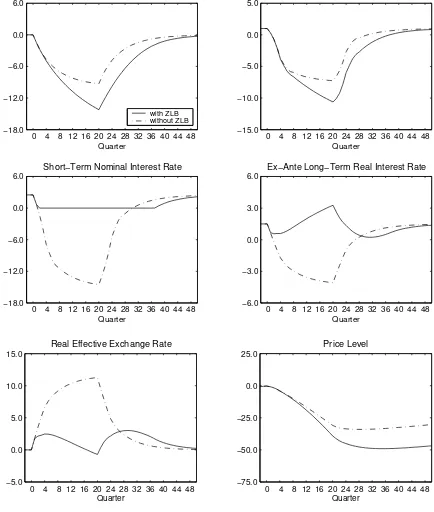
Figure 1 compares the outcome of this sequence of contractionary and deflationary
shocks when the zero bound is imposed explicitly (solid line) to the case when the zero
bound is disregarded and the nominal interest rate is allowed to go negative (dashed-dotted
line). As indicated by the dashed-dotted line, the central bank would like to respond to the
onset of recession and disinflation by drastically lowering nominal interest rates. If this were
possible, that is, if interest rates were not constrained at zero, the long-term real interest
rate would decline by about 4% and the central bank would be able to contain the output
gap and deflation around -9% and -8%, respectively. The reduction in nominal interest
rates would be accompanied by a 11% real depreciation of the currency in trade-weighted
6Orphanides and Wieland (2000) illustrate this point using recent data for Japan. For a further discussion
of the relationship of money and interest rates near zero we refer the reader to that paper.
7Of course, the likelihood of such a sequence of severe shocks is extremely small. We have chosen this
Figure 1: A Severe Recession and Deflation in Japan: Estimated Model
0 4 8 12 16 20 24 28 32 36 40 44 48 −18.0
−12.0 −6.0 0.0 6.0
Output Gap
Quarter
with ZLB without ZLB
0 4 8 12 16 20 24 28 32 36 40 44 48 −15.0
−10.0 −5.0 0.0 5.0
Annual Inflation
Quarter
0 4 8 12 16 20 24 28 32 36 40 44 48 −18.0
−12.0 −6.0 0.0 6.0
Short−Term Nominal Interest Rate
Quarter
0 4 8 12 16 20 24 28 32 36 40 44 48 −6.0
−3.0 0.0 3.0 6.0
Ex−Ante Long−Term Real Interest Rate
Quarter
0 4 8 12 16 20 24 28 32 36 40 44 48 −5.0
0.0 5.0 10.0 15.0
Real Effective Exchange Rate
Quarter
0 4 8 12 16 20 24 28 32 36 40 44 48 −75.0
−50.0 −25.0 0.0 25.0
Price Level
terms.
However, once the zero lower bound is enforced, the recessionary and deflationary shocks
throw the Japanese economy into a liquidity trap. Nominal interest rates are constrained at
zero for almost a decade. Deflation leads to increases in the long-term real interest rate up
to 4%. As a result, Japan experiences a double-digit recession that lasts substantially longer
than in the absence of the zero bound. Rather than depreciating, the currency temporarily
appreciates in real terms. The economy only returns slowly to steady state once the shocks
subside.
It is important to emphasize that in this scenario expectations of future inflation are
sufficient to return the economy ultimately to steady state. In this sense, the long period of
zero interest rates shown above does not represent a trap from which no escape is possible
but rather a long period of reduced policy effectiveness. Of course, it is well-known that
the model with the zero bound, as presented so far in Table A in the appendix would
be globally unstable. Once shocks to aggregate demand and/or supply push the economy
into a sufficiently deep deflation, a zero-interest-rate policy may not be able to return the
economy to the original equilibrium and a deflationary spiral would result. However, the
sequence of extreme shocks simulated above was still not sufficient to reach this point of no
return in our model of the Japanese economy.8
3
Exchange-rate peg versus price-level targeting
Svensson (2001) offers what he calls a foolproof way of escaping from a liquidity trap. With
interest rates constrained at zero and ongoing deflation he recommends that the central bank
stimulates the economy and raises inflationary expectations by switching to an
exchange-rate peg at a substantially devalued exchange exchange-rate and announcing a price-level target path.
8There would be a number of ways to resolve this global instability. For example Orphanides and
The exchange-rate peg is intended to be temporary and should be abandoned in favor of
price-level or inflation targeting when the price-level target is reached. Svensson delineates
the concrete proposal as follows:
• Announce an upward-sloping price-level target path for the domestic price level,
p∗
t = p∗t0+ 0.25π∗(t−t0), t≥t0 (2)
withp∗
t0 > pt0 and π∗>0;
• announce that the domestic currency will be devalued and that the nominal exchange
rate,s(ti,j), will be pegged to a fixed or possibly crawling exchange-rate target,
st(i,j) = ¯st(i,j), t≥t0 (3)
where ¯s(ti,j)= ¯s(t0i,j)+0.25 (π∗,(i)−π∗,(j)) (t−t
0) and the superscripts (i, j) are intended
to refer to the economies concerned;
• announce that, when the price-level target path has been reached, the peg will be
abandoned, either in favor of price-level targeting or inflation targeting with the same
inflation target.
This will result in a temporary crawling or fixed peg depending on the difference between
domestic and foreign target inflation rates. Svensson combines the exchange-rate peg with
a switch to price-level targeting because he expects the latter to stimulate inflationary
expectations more strongly than an inflation target. Further below we will investigate the
effectiveness of price-level targeting alone without the exchange-rate peg.
Svensson emphasizes that the central bank should be able to enforce the peg at a
deval-ued rate by standing ready to buy up foreign currency at this rate to an unlimited extent
if necessary. This will be possible because the central bank can supply whatever amount
of domestic currency is needed to buy foreign currency at the pegged exchange rate. This
situation differs from the defense of an overvalued exchange rate, which requires selling
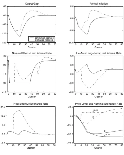
Figure 2: Switch from Taylor Rule to Exchange-Rate Peg
0 10 20 30 40 50 60 70 80 −18.0 −12.0 −6.0 0.0 6.0 Output Gap Quarter benchmark scenario exchange−rate peg
0 10 20 30 40 50 60 70 80 −16.0 −8.0 0.0 8.0 Annual Inflation Quarter
0 10 20 30 40 50 60 70 80 −1.0
0.0 1.0 2.0 3.0
Nominal Short−Term Interest Rate
Quarter
0 10 20 30 40 50 60 70 80 −6.0
−3.0 0.0 3.0 6.0
Ex−Ante Long−Term Real Interest Rate
Quarter
0 10 20 30 40 50 60 70 80 −8.0
0.0 8.0 16.0 24.0
Real Effective Exchange Rate
Quarter
0 10 20 30 40 50 60 70 80 −75.0
−50.0 −25.0 0.0 25.0
Price Level and Nominal Exchange Rate
s(JA,US)
p
p
s(JA,US)
We investigate the consequences of Svensson’s proposal if it is adopted during the severe
recession and deflation scenario after the central bank has observed 9 quarters of zero
nominal interest rates. The outcome is shown in Figure 2. The solid line in each panel
repeats the benchmark scenario fromFigure 1 where the central bank sticks with Taylor’s
rule. The dashed-dotted line indicates the outcome under Svensson’s proposal. We assume
that the central bank adopts the proposal in the 11th period of the simulation. Important
choice variables are the initial price level of the implied target path, the extent of the
devaluation and the length of the peg.
The peg is implemented with respect to the bilateral nominal exchange rate of the
Japanese Yen vis-`a-vis the U.S. Dollar. The implied devaluation and the associated
price-level target path are shown in the lower-right panel ofFigure 2. The nominal devaluation
results in a 15% real depreciation in the trade-weighted exchange rate. The peg delivers
the intended results. Inflationary expectations are jump-started and rise very quickly. The
real interest rate declines very rapidly, and the economy recovers from recession.
The uncovered-interest-parity condition and exchange-rate expectations play a key role.
Once the central bank announces the fixed peg the expected exchange-rate change is zero
and the nominal interest rate rises to the level of the foreign nominal interest rate absent any
foreign-exchange risk premium. The middle-left panel shows that the nominal interest rate
jumps to a positive level immediately upon the start of the peg as required by uncovered
interest parity.9
The preceding analysis of Svensson’s proposed exchange-rate peg emphasizes that
es-caping from the liquidity trap requires generating expectations of inflation. However, the
exchange-rate peg is not a necessary ingredient. Already Krugman (1998) pointed out that
inflationary expectations can be achieved by inducing expectations of future policy easing.
Using a model with staggered price contracts of fixed duration, Wolman (1998) showed that
9We avoided a return to zero interest rates by fine-tuning the length of the peg, the size of the devaluation
such expectations can be induced by implementing a policy rule that keeps the price level
trend-stationary. More recently, Eggertsson and Woodford (2003) analyze the possibility of
managing expectations regarding future policy easing in a model with imperfect competition
and random-duration Calvo-style price contracts. Eggertsson and Woodford (2003) show
that it is optimal for the central bank to commit to keeping nominal interest rates lower in
the future in order to affect expectations of inflation while the zero bound is still binding.
Eggertsson and Woodford also show that the optimal policy can be implemented through
commitment to a history-dependent rule using a price-level target that evolves over time.
Furthermore, they find that a simpler rule with a fixed price-level target achieves most of
the benefits of the optimal policy.
The four-quarter Taylor-style contracts in the Japan block of our macroeconometric
model imply a still greater degree of inflation persistence than the Calvo-style contracts
considered by Eggertsson and Woodford (2003). Inspired by their findings we investigate
whether switching to a price-level target alone would be sufficient to stimulate inflationary
expectations in our estimated model. More precisely, we consider the performance of the
following policy proposal:
• Announce an upward-sloping price-level target path for the domestic price level,
p∗
t = p∗t0+ 0.25π∗(t−t0), t≥t0
withp∗
t0 > pt0 and π
∗>0;
• replace the inflation target in the Taylor rule (equation (1)) with the above price-level
target and, thus, commit to lower interest rates in the future until the price gap is
completely closed.
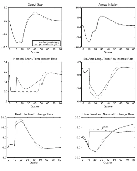
Figure 3 compares the performance of the Japanese economy in our model when the
central bank switches to the price-level target (dash-dotted line) after 9 quarters of zero
interest rates with the switch to the exchange-rate peg (solid line). Surprisingly, switching
Figure 3: Switch from Taylor Rule with Inflation Target to Price-Level Target
0 10 20 30 40 50 60 70 80 −12.0
−6.0 0.0 6.0
Output Gap
Quarter
exchange−rate peg price−level target
0 10 20 30 40 50 60 70 80 −10.0
−5.0 0.0 5.0 10.0
Annual Inflation
Quarter
0 10 20 30 40 50 60 70 80 −1.5
0.0 1.5 3.0 4.5
Nominal Short−Term Interest Rate
Quarter
0 10 20 30 40 50 60 70 80 −6.0
−3.0 0.0 3.0
Ex−Ante Long−Term Real Interest Rate
Quarter
0 10 20 30 40 50 60 70 80 −8.0
0.0 8.0 16.0 24.0
Real Effective Exchange Rate
Quarter
0 10 20 30 40 50 60 70 80 −30.0
−15.0 0.0 15.0 30.0
Price Level and Nominal Exchange Rate
s(JA,US)
p
exchange-rate peg. As shown in the two top panels output and inflation return to steady
state even a little bit faster than under the exchange-rate peg, the reason being that the
nominal interest rate remains at zero much longer and consequently the long-term real rate
falls lower and the real depreciation is a bit larger than under the exchange-rate peg.
4
Microeconomic foundations
The strength of the estimated three-country model of Coenen and Wieland (2002) lies in
its ability to match the observed degree of persistence of output and inflation in Japan,
the U.S. and the euro area. However, the model differs from a standard New-Keynesian
micro-founded model in several ways, most importantly because lags of the output gap
are included in the behavioral demand equations. To further gauge the validity of our
results from a theoretical perspective we simulate a recession and deflation scenario in the
micro-founded two-country model of Benigno and Benigno (2001).10
We start from the log-linear approximation derived by Benigno and Benigno and
imple-ment the zero bound in the same manner as in the estimated three-country model. Then,
we proceed to simulate a combination of government spending (-3 percentage points) and
productivity shocks (2 percentage points) that induce a negative output gap and deflation.
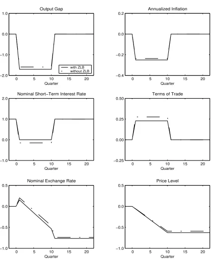
The outcome of this simulation is shown inFigure 4. We obtain results that are
qualita-tively similar to those for our estimated three-country model as far as the effect of the zero
bound on output, inflation and interest rates is concerned. However, the effect of the zero
bound is rather small and the dynamics of the micro-founded model are highly stylized due
to the lack of intrinsic persistence.11
We take this finding as a further corroboration of the results obtained in the estimated
model from a theoretical perspective.12 We do not follow the practice of adding ad-hoc serial
correlation to the shocks in this type of model so as to obtain empirically more plausible
10The model is described in more detail in Appendix A.2.
11We have simulated white-noise shocks without any ad-hoc serial correlation.
12Note that we intend to explore alternative shock combinations that may result in a more dramatic effect
Figure 4: The Effect of the Zero Bound in the Micro-Founded Model
0 5 10 15 20 −2.0
−1.0 0.0 1.0
Output Gap
Quarter
with ZLB without ZLB
0 5 10 15 20 −0.4
−0.2 0.0 0.2
Annualized Inflation
Quarter
0 5 10 15 20 −1.0
0.0 1.0 2.0
Nominal Short−Term Interest Rate
Quarter
0 5 10 15 20 −0.25
0.00 0.25 0.50
Terms of Trade
Quarter
0 5 10 15 20 −1.0
−0.5 0.0 0.5
Nominal Exchange Rate
Quarter
0 5 10 15 20 −1.0
−0.5 0.0 0.5
Price Level
impulse responses.13 In the appendix, we provide additional figures of simulations, which
show that the hoped-for benefits of a switch to an exchange-rate peg or to a price-level
target also obtain in the micro-founded model (cf.Figures A and B in Appendix A.3).
5
Implications of imperfect credibility
So far, exchange-rate-based and price-level-target-based approaches appear equally effective
in inducing inflationary expectations in a liquidity trap. From a practical perspective,
however, there is an important difference. While the exchange-rate peg can be verified
every day that the central bank maintains it, the price-level target path announced by the
central bank and the resulting price gap are not directly observable by the public. Thus, the
success of price-level targeting may depend particularly on the credibility of the announced
target path.
To gauge the validity of our findings from a practical perspective, we consider an
alterna-tive scenario, in which a shareλof market participants trust the central bank’s commitment
to a price-level target (0 ≤ λ≤ 1) while the others remain skeptical regarding the policy
switch (1−λ). Skeptical market participants still believe that the central bank will pursue
an inflation target rather than a price-level target. In other words, they do not believe that
the central bank intends to induce sufficient inflation in the future to fully make up the
price-level gap. We assume that the share λ of market participants that trust the central
bank converges to 1 at an exponential rate.
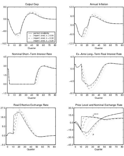
We report the outcomes for alternative values of λinFigure 5. The solid line repeats
the scenario fromFigure 3with a perfectly credible switch to a price-level target (λ= 1).
Alternatively, we consider values of 0.5 (dashed-dotted line), 0.3 (dashed line) and 0.2
(dotted line). The results we obtain indicate that the benefits of a switch to price-level
targeting are reduced substantially if more than half of the market participants do not
immediately believe the central bank’s announcement.
13The ongoing research program that involves adding further frictions to the model to improve the
Figure 5: Imperfect Credibility of the Price-Level Target: Estimated Model
0 10 20 30 40 50 60 70 80 −16.0 −8.0 0.0 8.0 Output Gap Quarter perfect credibility imperf. cred.: λ = 0.50 imperf. cred.: λ = 0.30 imperf. cred.: λ = 0.20
0 10 20 30 40 50 60 70 80 −12.0 −6.0 0.0 6.0 12.0 Annual Inflation Quarter
0 10 20 30 40 50 60 70 80 −1.5
0.0 1.5 3.0 4.5
Nominal Short−Term Interest Rate
Quarter
0 10 20 30 40 50 60 70 80 −8.0
−4.0 0.0 4.0
Ex−Ante Long−Term Real Interest Rate
Quarter
0 10 20 30 40 50 60 70 80 −9.0
0.0 9.0 18.0 27.0
Real Effective Exchange Rate
Quarter
0 10 20 30 40 50 60 70 80 −45.0 −30.0 −15.0 0.0 15.0 30.0
Price Level and Nominal Exchange Rate
s(JA,US)
p
6
Conclusions
Using an estimated three-country model we have found that the zero bound on nominal
interest rates significantly worsens the macroeconomic performance of the Japanese economy
in a recession and deflation scenario. Even though nominal interest rates are constrained at
zero, the central bank may improve performance substantially by devaluing the exchange
rate and switching to an exchange-rate peg or by committing to a price-level target path
and an interest-rate rule that will close the price gap in the future. A similar analysis
in a more stylized micro-founded model reinforces the plausibility of these findings from
a theoretical perspective. From a practical perspective, however, lack of credibility may
References
Adam, K. and R. M. Billi, 2003, Optimal monetary policy under commitment with a zero bound on nominal interest rates, unpublished manuscript, University of Frankfurt, Decem-ber.
Benhabib, J., S. Schmitt-Groh´e and M. Uribe, 2002, Avoiding liquidity traps, Journal of Political Economy, 110, 535-563.
Benigno, G. and P. Benigno, 2001, Monetary policy rules and the exchange rate, CEPR Dicsussion Paper No. 2807, May.
Bernanke, B., 2002, Deflation: Making sure “It” doesn’t happen here, Speech before the National Economists Club, Washington D.C., November 21, 2002.
Buiter, W. H., 2001, The liquidity trap in an open economy, CEPR Discussion Paper, DP 2923.
Buiter, W. H. and I. Jewitt, 1981, Staggered wage setting with real wage relativities: Vari-ations on a theme of Taylor, The Manchester School, 49, 211-228, reprinted in W. H. Buiter (ed.), 1989, Macroeconomic theory and stabilization policy, Manchester: Manchester Uni-versity Press.
Buiter, W. H. and N. Panigirtzoglou, 1999, Liquidity traps: How to avoid them and how to escape them, unpublished manuscript, March.
Boucekkine, R., 1995, An alternative methodology for solving nonlinear forward-looking models, Journal of Economic Dynamics and Control, 19, 771-734.
Calvo, G. A., 1983, Staggered prices in a utility-maximizing framework, Journal of Monetary Economics, 12, 383-398.
Clouse, J., D. Henderson, A. Orphanides, D. Small, and P. Tinsley, 2000, Monetary policy when the nominal short-term interest rate is zero, Finance and Economics Discussion Series, 2000-51, Board of Governors of the Federal Reserve System, November.
Coenen, G. and V. Wieland, 2002, Inflation dynamics and international linkages: A model of the United States, the euro area and Japan, ECB Working Paper No. 181, September.
Coenen, G. and V. Wieland, 2003, The zero-interest-rate bound and the role of the exchange rate for monetary policy in Japan, Journal of Monetary Economics, 50(5), 1071-1101.
Dornbusch, R., 1980, Exchange-rate economics: Where do we stand?, Brookings Papers on Economic Activity, 3, 537-584.
Dornbusch, R., 1987, Exchange-rate economics: 1986, Econonomic Journal, 97, 1-18.
irresponsible, IMF Working Paper No. 03/64, March.
Eggertsson, G. B. and M. Woodford, 2003, The zero bound on interest rates and optimal monetary policy, Brookings Papers on Economic Activity, 1, 139-233.
Fair, R. and J. B. Taylor, 1983, Solution and maximum likelihood estimation of dynamic nonlinear rational expectations models, Econometrica, 51, 1169-1185.
Fuhrer, J. C. and B. F. Madigan, 1997, Monetary policy when interest rates are bounded at zero, Review of Economics and Statistics, 79, 573-585.
Fuhrer, J. C. and G. R. Moore, 1995a, Inflation persistence, Quarterly Journal of Economics, 110, 127-159.
Fuhrer, J. C. and G. R. Moore, 1995b, Monetary policy trade-offs and the correlation between nominal interest rates and real output, American Economic Review, 85, 219-239.
Goodfriend, M., 2000, Overcoming the zero bound on interest rate policy, Journal of Money, Credit and Banking, 32, 1007-1035.
Hunt, B. and D. Laxton, 2001, The zero interest rate floor and its implications for monetary policy in Japan, IMF Working Paper, WP/01/186, International Monetary Fund.
Johnson, K., D. Small and R. Tryon, 1999, Monetary policy and price stability, Federal Reserve Board, International Finance Discussion Paper 1999-641, July.
Juillard, M., 1994, DYNARE - A program for the resolution of non-linear models with forward-looking variables, Release 1.1, mimeo, CEPREMAP.
Krugman, P., 1998, It’s baaack: Japan’s slump and the return of the liquidity trap, Brook-ings Papers on Economic Activity, 2, 137-187.
Laffargue, J., 1990, R´esolution d’un mod`ele macro´economique avec anticipations ra-tionnelles, Annales d’Economie et de Statistique, 17, 97-119.
Laxton, D. and E. Prasad, 1997, Possible effects of European Monetary Union on Switzer-land: A case study of policy dilemmas caused by low inflation and the nominal interest rate floor, IMF Working paper, WP/97/23, International Monetary Fund.
McCallum, B. T., 2000, Theoretical analysis regarding a zero lower bound on nominal interest rates, Journal of Money, Credit and Banking, 32, 870-904.
McCallum, B. T., 2002, Inflation targeting and the liquidity trap, in N. Loayza and R. Soto (eds.), Inflation targeting: design, performance, challenges, Santiago: Central Bank of Chile.
Meltzer, A., 1998, Time to print money, Financial Times, July 17.
Orphanides, A. and V. Wieland, 1998, Price stability and monetary policy effectiveness when nominal interest rates are bounded at zero, Finance and Economics Discussion Series, 98-35, Board of Governors of the Federal Reserve System, June.
Orphanides, A. and V. Wieland, 2000, Efficient monetary policy design near price stability, Journal of the Japanese and International Economies, 14, 327-365.
Posen, A., 1998, Restoring Japan’s economic growth, Institute for International Economics, Washington D.C..
Reifschneider, D. and J. C. Williams, 2000, Three lessons for monetary policy in a low inflation era, Journal of Money, Credit and Banking, 32, 936-966.
Svensson, L. E. O., 2001, The zero bound in an open-economy: A foolproof way of escaping from a liquidity trap, Monetary and Economic Studies, 19, 277-312.
Svensson, L. E. O., 2002, Escaping from a liquidity trap and deflation: The foolproof way and others, Journal of Economic Perspectives, forthcoming.
Svensson, L. E. O., 2003, The magic of the exchange rate: Optimal escape from a liquidity trap in small and large open economies, unpublished manuscript, Princeton University, December.
Taylor, J. B., 1980, Aggregate dynamics and staggered contracts, Journal of Political Econ-omy, 88, 1-24.
Taylor, J. B., 1993a, Macroeconomic policy in the world economy: From econometric design to practical operation, New York: W.W. Norton.
Taylor, J. B., 1993b, Discretion versus policy rules in practice, Carnegie-Rochester Confer-ence Series on Public Policy, 39, 195-214.
Wolman, A. L., 1998, Staggered price setting and the zero bound on nominal interest rates, Federal Reserve Bank of Richmond Quarterly, 84, 1-22.
Appendix
A.1 The model of Coenen and Wieland (2002)
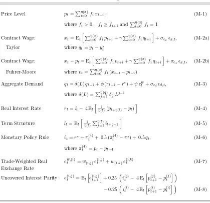
Table A provides an overview of the model. Due to the existence of staggered contracts,
the aggregate price level pt corresponds to the weighted average of wages on overlapping
contractsxt(equation (M-1) inTable A). The weightsfi(i= 1, . . . , η(x)) on contract wages
from different periods are assumed to be non-negative, non-increasing and time-invariant and need to sum to one. η(x) corresponds to the maximum contract length. Workers negotiate long-term contracts and compare the contract wage to past contracts that are still in effect and future contracts that will be negotiated over the life of this contract. As indicated by equation (M-2a), Taylor’s nominal wage contracting specification implies that the contract wage, xt, is negotiated with reference to the price level that is expected to
prevail over the life of the contract as well as the expected deviations of actual output from potential, qt. The sensitivity of contract wages to excess demand is measured by γ. The
contract-wage shock ǫx,t, which is assumed to be serially uncorrelated with zero mean and
unit variance, is scaled by the parameterσǫx.
The distinction between Taylor-style contracts and Fuhrer-Moore’s relative real-wage contracts concerns the definition of the wage indices that form the basis of the intertem-poral comparison underlying the determination of the current nominal contract wage. The Fuhrer-Moore specification assumes that workers negotiating their nominal wage compare the implied real wage with the real wages on overlapping contracts in the recent past and near future. As shown in equation (M-2b) in Table A the expected real wage under contracts signed in the current period is set with reference to the average real contract-wage index expected to prevail over the current and the next following quarters, where
vt=ηi=0(x) fi(xt−i−pt−i) refers to the average of real contract wages that are effective at
timet.
Output dynamics are described by the open-economy aggregate-demand equation (M-3), which relates the output gap to several lags of itself, to the lagged ex-ante long-term real interest rate rt−1 and to the trade-weighted real exchange rate ewt . The demand shockǫd,t
in equation (M-3) is assumed to be serially uncorrelated with mean zero and unit variance and is scaled with the parameterσǫd.
14
14A possible rationale for including lags of output is to account for habit persistence in consumption as well
Table A: Model Equations
Price Level pt=
η(x)
i=0 fixt−i, (M-1)
where fi>0, fi≥fi+1 andηi=0(x)fi= 1
Contract Wage: xt= Et
η(x)
i=0 fipt+i+γ η(x)
i=0 fiqt+i
+σǫxǫx,t, (M-2a)
Taylor where qt=yt−y∗t
Contract Wage: xt−pt= Et
η(x)
i=0 fivt+i+γ η(x)
i=0 fiqt+i
+σǫxǫx,t, (M-2b)
Fuhrer-Moore where vt=
η(x)
i=0 fi(xt−i−pt−i)
Aggregate Demand qt=δ(L)qt−1+φ(rt−1−r∗) +ψ e
w
t +σǫdǫd,t, (M-3)
where δ(L) =η(q)
j=1 δjLj−1
Real Interest Rate rt=lt− 4 Et
1
η(l)(pt+η(l)−pt)
(M-4)
Term Structure lt= Et
1
η(l)
η(l) j=1it+j−1
(M-5)
Monetary Policy Rule it=r∗+π
(4)
t + 0.5 (π
(4)
t −π∗) + 0.5qt, (M-6)
where πt(4)=pt−pt−4
Trade-Weighted Real ew,t (i)=w(i,j)e (i,j)
t +w(i,k)e (i,k)
t (M-7)
Exchange Rate
Uncovered Interest Parity e(ti,j)= Et
e(ti,j+1)
+ 0.25i(tj)− 4 Et
p(tj+1) −p (j)
t
−0.25i(ti)−4 Et
p(ti+1) −p (i)
t (M-8)
Notes: p: aggregate price level; x: nominal contract wage;q: output gap; y: actual output;y∗: potential output ǫx: contract wage shock; v: real contract wage index; r: ex-ante long-term real interest rate;
r∗: equilibrium real interest rate; ew
: trade-weighted real exchange rate; ǫd: aggregate demand shock;
l: long-term nominal interest rate;i: short-term nominal interest rate;π(4): annual inflation;π∗: inflation target;e: bilateral real exchange rate.
interest rate is usually considered the primary policy instrument of the central bank. As a benchmark for our analysis we assume that nominal interest rates in Japan, the United States and the euro area are set according to Taylor’s (1993b) rule (equation (M-6)) which implies a policy response to deviations of inflation from the central banks’s inflation target
π∗ and to deviations of actual output from potential.
The trade-weighted real exchange rate is defined by equation (M-7). The superscripts (i, j, k) are intended to refer to the economies within the model without being explicit about the respective economy concerned. Thus, e(i,j) represents the bilateral real exchange
rate between countries i and j, e(i,k) the bilateral real exchange rate between countries i
and k, and consequently equation (M-7) defines the trade-weighted real exchange rate for country i. The bilateral trade-weights are denoted by (w(i,j), w(i,k), . . .). Finally, equation (M-8) constitutes the uncovered-interest-parity condition with respect to the bilateral ex-change rate between countries iand j in real terms. It implies that the difference between today’s real exchange rate and the expectation of next quarter’s real exchange rate is set equal to the expected real interest rate differential between countriesjandi. Alternatively, we can allow the relative quantities of base money at home and abroad to have a direct effect on the exchange rate in addition to the effect of interest-rate differentials. Due to this so-called portfolio-balance effect, the bilateral exchange rate need not satisfy uncovered interest parity exactly.15
In the deterministic steady state of this model the output gap is zero and the long-term real interest rate equals its equilibrium valuer∗. The equilibrium value of the real exchange
rate is normalized to zero. Since the overlapping contracts specifications of the wage-price block do not impose any restriction on the steady-state inflation rate, it is determined by monetary policy alone and equals the target rate π∗ in the policy rule.
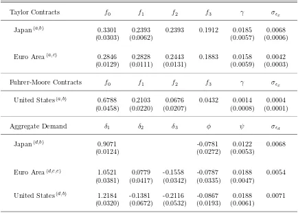
Parameter estimates for the preferred staggered-contracts specifications and the aggregate-demand equations are presented in Table B. For a more detailed discussion of these results we refer the reader to Coenen and Wieland (2002). The model fits historical output and inflation dynamics in the United States, the euro area and Japan quite well as indicated by the absence of significant serial correlation in the historical shocks (see Fig-ure 1 in Coenen and Wieland (2002)) and the finding that the autocorrelation functions of output and inflation implied by the three-country model are not significantly different from those implied by bivariate unconstrained VAR models (see Figure 2 in Coenen and Wieland (2002)).
15Such specification (cf. Dornbusch (1980, 1987)) is also considered by McCallum (2000) and Svensson
Table B: Parameter Estimates: Staggered Contracts and Aggregate Demand
Taylor Contracts f0 f1 f2 f3 γ σǫx
Japan(a,b) 0.3301 0.2393 0.2393 0.1912 0.0185 0.0068
(0.0303) (0.0062) (0.0057) (0.0006)
Euro Area(a,c) 0.2846 0.2828 0.2443 0.1883 0.0158 0.0042
(0.0129) (0.0111) (0.0131) (0.0059) (0.0003)
Fuhrer-Moore Contracts f0 f1 f2 f3 γ σǫx
United States(a,b) 0.6788 0.2103 0.0676 0.0432 0.0014 0.0004
(0.0458) (0.0220) (0.0207) (0.0008) (0.0001)
Aggregate Demand δ1 δ2 δ3 φ ψ σǫd
Japan(d,b) 0.9071 -0.0781 0.0122 0.0068
(0.0124) (0.0272) (0.0053)
Euro Area(d,c,e) 1.0521 0.0779 -0.1558 -0.0787 0.0188 0.0054
(0.0381) (0.0417) (0.0342) (0.0335) (0.0047)
United States(d,b) 1.2184 -0.1381 -0.2116 -0.0867 0.0188 0.0071
(0.0320) (0.0672) (0.0532) (0.0193) (0.0061)
Notes:(a)Simulation-based indirect estimates using a VAR(3) model of quarterly inflation and the output
gap as auxiliary model. Standard errors in parentheses. (b)
Output gap measure constructed using OECD data. (c)
Inflation in deviation from linear trend and and output in deviation from log-linear trend.
(d)GMM estimates using a constant, lagged values (up to order three) of the output gap, the quartely
inflation rate, the short-term nominal interest rate and the real effective exchange rate as instruments. In addition, current and lagged values (up to order two) of the foreign inflation and short-term nominal interest rates have been included in the instrument set. Robust standard errors in parentheses. (e) For
A.2 The model of Benigno and Benigno (2001)
Key features of the model
• The model assumes imperfect competition and nominal rigidities due to Calvo-style
contracts.
• There are many differentiated goods falling in two classes, home goods (H) and foreign
goods (F).
• Markets are complete and the law of one price holds. There is perfect risk sharing in
consumption.
• There are two types of shocks, government spending shocks (g) and productivity
shocks (a).
• Country-specific demand shocks and the terms of trade can create dispersion of output
across countries.
• We use symmetric parameter values taken from Benigno and Benigno (2001).
• Notation: Y (output), C (world consumption), S (nominal exchange rate), P
(pro-ducer price level),i(nominal interest rate), T =SPF/PH (terms of trade), π
(infla-tion),R (flex-price world real interest rate).
• Gaps concern the difference between actual values and flex-price equilibrium values.
Key equations
Home and foreign output:
YtH = (1−n)Tt+Ct+gHt
YF
t = −nTt+Ct+gFt
World output gap:
Et[ytW+1] = ytW +d1(iHt −Et[πtH+1]−Rt)
Terms of trade:
Tt = Tt−1+ ∆St+π
F t −πtH
Uncovered interest parity:
Et[∆St+1] = iHt −iFt
Home and foreign inflation:
πtH = k1Httt+kH2 ytW +kH3 Et[πHt+1]
πF
t = k1Fttt+k2FytW +k3FEt[πtF+1],
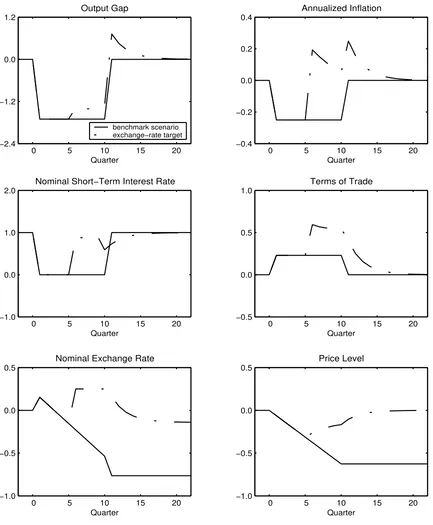
A.3 Additional simulation results for the micro-founded model
Figure A: Devaluation and Exchange-Rate Peg
0 5 10 15 20 −2.4
−1.2 0.0 1.2
Output Gap
Quarter
benchmark scenario exchange−rate target
0 5 10 15 20 −0.4
−0.2 0.0 0.2 0.4
Annualized Inflation
Quarter
0 5 10 15 20 −1.0
0.0 1.0 2.0
Nominal Short−Term Interest Rate
Quarter
0 5 10 15 20 −0.5
0.0 0.5 1.0
Terms of Trade
Quarter
0 5 10 15 20 −1.0
−0.5 0.0 0.5
Nominal Exchange Rate
Quarter
0 5 10 15 20 −1.0
−0.5 0.0 0.5
Price Level
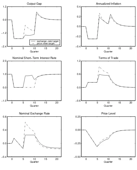
Figure B: Price-Level Targeting versus Exchange-Rate Peg
0 5 10 15 20 −2.4
−1.2 0.0 1.2
Output Gap
Quarter
exchange−rate target price−level target
0 5 10 15 20 −0.4
−0.2 0.0 0.2 0.4
Annualized Inflation
Quarter
0 5 10 15 20 −1.0
0.0 1.0 2.0
Nominal Short−Term Interest Rate
Quarter
0 5 10 15 20 −0.6
0.0 0.6 1.2
Terms of Trade
Quarter
0 5 10 15 20 −0.4
0.0 0.4 0.8
Nominal Exchange Rate
Quarter
0 5 10 15 20 −0.50
−0.25 0.00 0.25
Price Level