Data Envelopment Analysis with Functional Data using Preference Method

(1)

Data Envelopment Analysis with Functional Data using

Preference Method

Syyed Nima Hashemi

Ghermezi

Department of Industrial

Engineering, Faculty of Engineering, Islamic Azad University, Saveh Branch,

Saveh, Iran

Taher Taherian

Department of Industrial

Engineering, Faculty of Engineering, Islamic Azad University, Saveh Branch,

Saveh, Iran

Farhad Hosseinzadeh

Lotfi

Department of Mathematics, Science and Research Branch,

Islamic Azad University, Tehran, Iran

ABSTRACT

In this paper we assess the efficiency of units using data envelopment analysis (DEA). In first stage, a functional data is converted to a fuzzy bell shape number and then a benchmark point would be chosen for each input or output and using the preference ratio method, the equivalence multiplier of each data would be calculated. In order to simplification of functional data, functional data will be replaced bythe equivalence multiplier.

Keywords

Data envelopment analysis (DEA) ,fuzzy bell shape, Preference ratio.

1. INTRODUCTION

One of the ranking methods of fuzzy numbers is the preference ratio methodthat is presented by Modarres and Sadi-Nezhad(2001) [1]. Suppose A and B as two fuzzy numbers.S(A) and S(B) are defined as the support of A and B,separately and the supremum and infimum of S(A) and S(b) are shown as LA, UA, LB, UB, respectively. The Ω is defined below:

( ) ( )

And , the preference function is defined as follows:

B A, k ) (

) ( )

(  



U

L k U

k

dx x

dx x G





( ), is also defined as follows:

) ( ) ( B

) ( ) ( A ) ( p

  

  

 

  

B A

A B

G G

In other words, belongs to a fuzzy number whichits area ratio under itsmembership functionand after the point , to the total area under the membership function curve is more.

According the previous comments, the preference ration of A and B are defined as follows:







P( ) B



) ( R

A ) ( P

) ( R

A B

A A

       

 

B A

Which the symbol | | shows the interval lengths.

In other words, the fuzzy number with maximum distance from Ω will gain the upper rank.In order to rank the fuzzy numbers with the count more than two,Modarresand Sadi-Nezhad (2005) [2] developed an approachwherein all fuzzy numbers compared with abenchmark is investigated. They defined a benchmark for a set of triangular fuzzy numbers and compared each preference ratio of the numbers with them.In order to this comparison, they defined the equivalence and equivalence multiplieras follows:

In preference method, two fuzzy number A and B are equivalent ifR(A)=R(B)=0.5 and in this case, A=B. the equivalence multiplier is also defined as follows:

K is called the equivalence multiplier of A toward B, whenever KA=B.

Nowadays, DEA is also one of applicable ways to calculate the relation efficiency of units.

Charnes et al (1978) [3] presented the CCR model for first time. Theconstant return to scale is considered in this model. In other words, increasing the inputs caused increasing the outputs with the same ratio. Banker et al (1984)[4] presented the BCC method wherein the variable return to scale was considered.This means that, any changes in inputs don’t cause the changes in outputs with the same ratio.Since that time until now, data envelopment analysis is used and developed in many centers and organizations like banks, schools, universities, hospitals, insurance agencies, andfactories [5-14].Ranking the unitswas anotherdevelopmentof DEA that many papers have written about it. Andersen and Petersen (1993) [15]presented a procedure for ranking efficient units. They recalculated the efficiency of efficient units but this time in order to calculate the efficiency of a particular unit, that unit has been eliminated from production possibility set (PPS).

Another advance in DEA is bringing some changes about in type of inputs and outputs. Cook et al (1996) [16-17] presented DEA with ordering data and then in 1997 they considered some inputs sequentially. Cooper et al (1999) [18-19] investigated the interval data in DEA and presented a comprehensive form using the confidence interval concept and converted it to an equivalent linear programming through a set of scale conversions and change of variables and the efficiency value of each decision maker unit obtained from this model was deterministic, less or equal to 1.

(2)

helped to calculate the interval efficiency for each DMU in pessimistic and optimistic viewpoint. Their model was applicablefor deterministic data at the beginning but they developed their model to be included of interval and fuzzy data. The deficiency of their model was considering just one input and output and their model was using different efficient boundaries to measure efficiency intervals of different DMUs.

Guo and Tanaka (2001)[24], Kahraman and Tolga (1998)[25], Kao and Liu (2000)[26] introduced DEA with fuzzy data. In most important solution, they converted the fuzzy data into interval data per different .

2. MODEL DESCRIPTION

Assume n units aseach unit has m inputs and n outputs, are being probing and calculating their efficiency. Each unit of input of output has some functional data as each data give different values of dependent variable or response variable for different values of dependent variable. So practically, the data are presented as a set of order pair. Here we present two assumptions. First, the values of independent variableare equal in homological input or outputdata. The second, the weight and importance of these values are equal. For example, suppose that the data is evaluated in different periods with symmetric importance.Applying mentioned assumptions, we can just consider the response variables, so the data practically will be a set of single component numbersobtained in different periods.Now the purpose is calculating ofsuch units.Hereinafter, these data will be called, period data or period input and output.

3. CONVERTING A PERIOD DATA TO

A FUZZY DATA

In this section, we want to convert a period data to a bell shape fuzzy data. Thetypes of data are numbers obtained from different periods whilethe results originated from distinctperiods may bedifferent and in this situation, it sounds that the data may be irrational numbers so functional data could be converted to a fuzzy number by defining a value function.It's clear that each data is a quantitative value of a quality in different periods. It’s clear that, in a period data, each number which demonstrates a quality with more realitywill have more valueso the average of a period data must have the maximum value and whateverit'smovedaway from the mean the value assigned to the number willbe less value. Here the bell shape fuzzy number could be used for each period data that is very similar to a normal distribution with a difference that the area under the distribution curve is equal to √ . Assume m as the mean and as the standard deviation of a period data, the bell shape function will be

defined as ( ) ( ( ) ), but the problem is that the

numbers located out of the data area will also have a value even if this value may belittle.So this function will change as follows:             b b a a x 0 x ) 2 ) m x ( ( EXP x 0 ) x ( ₂ 2





Here, a and b are the minimum and maximum value of each period data respectively.Hereinafter, the mentioned function is

called, restricted bell shape (RBS) function and It will be shown with (a,m,b, ).

Fig 1: Restricted bell shape function

4. EQUIVALENCE MULTIPLIER

CALCULATION

If we want to compare some fuzzy numbers, it may sound that a pairwise comparison can be useful but it’s not practical because being greater in preference method, doesn’t have transitive property and this means if we want to compare three fuzzy numbers, A, B and C, if A is greater than B and B is greater than C, A may be less than C.to be obvious, there is a counterexample. Assume that A, B and C are three RBS fuzzy numbers: C A C B B A                  _ _     0.7799 R(C) 0.2202 R(A) 0.4751 R(C) 0.5250 R(B) 0.4960 R(B) 0.5041 R(A) 0.4010) 3.4000 0.9982 (0.5490 C 0.3987) 3.7879 0.9968 (0.5981 B ) 4000 0. 4.0000 1.0000 (0.5000 = A

As it can be seen, A is greater than B and B greater than C but A is not greater than C so the transitive property can’t be confirmed. To solve this problem, we compare all fuzzy numbers with a benchmark number and the equivalence multiplier of the benchmark will be calculated with respect to all numbers.

Now two algorithms are being presented. First algorithm, calculates the preference ratio of two RBS number and the second algorithm calculates the equivalence multiplier in respect of one RBS number.

Notice that, in first algorithm, ( )shows the cumulative normal distributionthat help us to calculate the integral of RBS membership function because it’s obvious that if (L, M, U, σ) is a RBS number we have:

     _                _  



) ( ) ( ) ( ) ( ) ( ) ( (X) G ) ( ) ( 2 ) ( RBS 2                  M L M U M X M U dx x dx x M X M U dX X U L RBS U RBS U X RBS Algorithm 1:

Assume two fuzzy numbers A and B.

A= ( , , , ) and B= ( , , , )

(3)

Put L=min ( , ) , U=max ( , ) , , i=L, G(A)=0 , G(B)=0.

Step 2:

If go to step 6 else go to next step

Step 3:

If then put A= 1

If then put A= 0

If put ₍₍ (( ₎₎)) _{) ((}) (( ) ₎)) ₎₎

Step 4:

If then put B= 1

If then put B= 0

If put (( )) ) (( ) ))

(( )) ) (( ) ))

Step5:

If then put ( ) ( )

If then put ( ) ( ) , ( ) ( )

Add e units to I and go to step 6.

Step 6:

( ) ( ( )

) ( ) (

( )

)

If (x, y, z, ) is a RBS number, we define :

( ) ( ), it’s true, because when all of

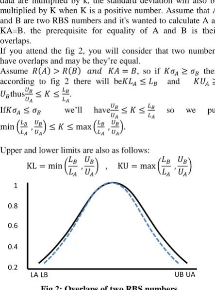
data are multiplied by k, the standard deviation will also be multiplied by K when K is a positive number. Assume that A and B are two RBS numbers and it's wanted to calculate A as KA=B. the prerequisite for equality of A and B is their overlaps.

If you attend the fig 2, you will consider that two numbers have overlaps and may be they’re equal.

Assume ( ) ( ) , so if then according to fig 2 there will be and

thus .

If we’ll have so we put

( ) ( )

Upper and lower limits are also as follows:

[image:3.595.54.276.379.677.2]

( ) ( )

Fig 2: Overlaps of two RBS numbers

Algorithm 2 is used to calculate K for the RBS number A with respect to B.

Algorithm 2: finding the equivalence multiplier of A with respect to B.

Step 1:

Put switch=0 ,apply algorithm 1 for A and B.

If , put and algorithm 2 is finished.

If , swap A and B and put switch=1.

Step 2:

Put ( ) ( )

,

Step 3:

Apply algorithm 1 for A and B and

.

Step 4:

If the difference between R( ) and 0.5 is less than e then go to step 8 else, go to next step.

Step 5:

If R( ) then put If R( ) then put

Step 6: Put

Step 7:

Apply algorithm 1 for A and B and and return to step 3.

Step 8:

If switch=0 then put else .

In data envelopment analysis, we consider a benchmark point for each input and output which they are the period data. Suppose RBS numbers,( )and

( ) are the ithinput related to jthoutput

respectively as the first component to fourth, are the minimum value, mean, maximum value and standard deviation, separately.

Also assume ( ) and ( ) as a benchmark for ithinput and jth output.

It's obvious that ( ) ( ) because when all data are multiplied by K, the standard deviation is also be multiplied by K.

To calculate the preference ratio algorithm 1 can be used used and to gain the equivalence multiplier algorithm 2 can be used.

Now the preference method is applied for all of inputs and outputs and we find the equivalence multiplier of benchmarks with respect to related data. Model P1 is a CCR model with RBS data.

n 1,..., j 0

λ

s 1,..., r ) ys , yu , ym , (yl ) ys , yu , ym , (yl λ

m 1,..., i ) xs , xu , xm , (xl θ ) xs , xu , xm , (xl λ

st

θ min θ : p

j n

1 j

rp rp rp rp rj rj rj rj j n

1 j

ip ip ip ip ij ij ij ij j p 1

 

 





 

Model P2 can be obtained using two assumptions:

is the equivalence multiplier of

benchmark( )with respect

to( ).

is the equivalence multiplier of

benchmark( )with respect

to( ).

UA 0.2

1

0.6

0.4 0.8

(4)

n 1,..., j 0

λ

s 1,..., r ) ys , yu , ym , (yl K ) ys , yu , ym , (yl K λ

m 1,..., i ) xs , xu , xm , (xl K θ ) xs , xu , xm , (xl K λ

st

θ min θ : p

j n

1 j

r r r r rp Y r r r r rj Y j n

1 j

i i i i ip X i i i i ij X j

p 2

 

 





 

It’s obvious that by changing the benchmark, many models can be derived. With simplification of model, P2 is changed to model P3 that is a simple CCR model.

n 1,..., j 0

λ

s 1,..., r K K λ

m 1,..., i K θ K λ

st

θ min θ : p

j n

1 j

rp Y rj Y j n

1 j

ip X ij X j

p 3

 

 





 

Now the main question is what the best benchmark is. Suppose are some fuzzy numbers that the benchmark A is chosen for them randomly. Following attributes areindefeasible:

1- In the equation , if ( )> ( ) then else

2- If ( ) ( ) then all of equivalence

multipliers are greater than 1 and if

( ) ( ), the equivalence multipliers are

less than 1.

if ( ) ( ) ( )then some of equivalence multipliers are less and some are more than 1.

3- If ( ) ( ).

4- Whatever k is closer to 1, it demonstrates the proximity of fuzzy number and the benchmark.

According to previous notes, each benchmark could be chosen but to have a better analysis, it seems that, it’s better to select the best benchmark; in this case, all numbers will be greater than1 or they are less than 1 and the advantage is closeness to 1.

In DEA, between inputs, it seems that the best benchmarkis the minimum benchmark and between outputs the best is the maximum so the benchmark selection procedure is as follows: For each ith_{input like}₍

), the benchmark

will be( ) in which we will have:

,

The reason of thisselectionfor standard deviation is that in normal distribution and some distributions like normal, 99.73 percent of data are in an interval with 6 standard deviation length.

For each output, the benchmark is( ) that we will have:

,

Of course, it’s obvious that, otherbenchmarks can be existed.

5. NUMERICAL EXAMPLE

Table 1 shows the data for 5 units as RBS numbers.

Table 1. The data for an example

Unit1 Unit2 Unit3 Unit4 Unit5

Input1 (3.5,4.0,4.5,0.16) (2.9,3.0,3.1,0.03) (4.4,4.9,5.4,0.16) (3.4,4.1,4.8,0.23) (5.9,6.5,7.1,0.2)

Input2 (1.9,2.1,2.3,0.06) (1.4,1.5,1.6,0.03) (2.2,2.6,3.0,0.13) (2.1,2.3,2.5,0.06) (3.6,4.1,4.6,0.16)

Output1 (2.4,2.6,2.8,.06) (2.2,2.4,2.7,0.08) (2.7,3.2,3.7,0.16) (2.5,2.9,3.3,0.13) (4.4,5.1,5.8,0.23)

Output2 (3.8,4.1,4.4,0.1) (3.3,3.5,3.7,0.06) (4.3,5.1,5.9,0.27) (5.5,5.7,5.9,0.06) (6.5,7.4,8.3,0.3)

In table 2, some benchmarks have chosen for inputs and outputs. The first benchmark has selected the minimum between inputs and maximum between outputs. The second benchmark isalways the maximum value of inputs and

outputs. The third benchmark considered the minimum value of inputs or outputs and the fourth, has used the random numbers as a benchmark.

Table 2.The Benchmarks

Min-max Max Min Random

(2.9,3.0,3.1,0.03) (5.9,6.5,7.1,0.2) (2.9,3.0,3.1,0.03) (3.6675,4.3561,5.8010,0.3667)

(1.4,1.5,1.6,0.03) (3.6,4.1,4.6,0.16) (1.4,1.5,1.6,0.03) (1.9810,3.1924,3.8551,0.3033)

(4.4,5.1,5.8,0.23) (4.4,5.1,5.8,0.23) (2.2,2.4,2.7,0.08) (3.0024, 4.1074,4.2094,0.2022)

(6.5,7.4,8.3,0.3) (6.5,7.4,8.3,0.3) (3.3,3.5,3.7,0.06) (4.1912,5.6328,8.1045,0.6517)

(5)

Table 3. Min-Max benchmark

Unit1 Unit2 Unit3 Unit4 Unit5

Input1 1.3334 1.0000 1.6334 1.3667 2.1667

Input2 1.4001 1.0000 1.7334 1.5333 2.7335

Output1 0.5099 0.4757 0.6275 0.5686 1.0000

Output2 0.5540 0.4730 0.6892 0.7703 1.0000

CCR-input

oriented 0.8334 1.0000 0.8410 1.0000 0.9724

BCC-input

oriented 0.8345 1.0000 0.9071 1.0000 1.0000

CCR-output

oriented 0.8334 1.0000 0.8410 1.0000 0.9724

BCC-output

oriented 0.8804 1.0000 0,9300 1.0000 1.0000

Table 4. Max benchmark

Input1 0.6154 0.4616 0.7538 0.6309 1.0000

Input2 0.5122 0.3658 0.6341 0.5610 1.0000

Output1 0.5099 0.4757 0.6275 0.5686 1.0000

Output2 0.5540 0.4730 0.6892 0.7703 1.0000

CCR-input oriented

0.8335 1.0000 0.8412 1.0000 0.9726

BCC-input oriented

0.8346 1.0000 0.9072 1.0000 1.0000

CCR-output oriented

0.8335 1.0000 0.8412 1.0000 1.0000

BCC-output oriented

0.8804 1.0000 0.9301 1.0000 1.0000

Table 5.Min benchmark

Input1 1.3334 1.0000 1.6334 1.3667 2.1667

Input2 1.4001 1.0000 1.7334 1.5333 2.7335

Output1 1.0683 1.0000 1.3189 1.1953 2.1020

Output2 1.1714 1.0000 1.4573 1.6285 2.1145

CCR-input oriented

0.8318 1.0000 0.8410 1.0000 0.9724

BCC-input oriented

0.8327 1.0000 0.9071 1.0000 1.0000

CCR-output oriented

0.8318 1.0000 0.8410 1.0000 0.9724

BCC-output oriented

0.8785 1.0000 0.93 1.0000 1.0000

Table 6.Random benchmark

Input1 0.8598 0.6368 1.0498 0.8868 1.3908

Input2 0.7113 0.5099 0.8742 0.7799 1.3847

Output1 0.7064 0.6560 0.8594 0.7786 1.3691

Output2 0.6722 0.5730 0.8441 0.9310 1.2202

CCR-input oriented

0.8310 1.0000 0.8411 1.0000 0.9647

BCC-input oriented

0.8402 1.0000 0.9167 1.0000 1.0000

CCR-output oriented

0.8310 1.0000 0.8411 1.0000 0.9647

BCC-output oriented

08858 1.0000 0.9371 1.0000 1.0000

The efficiency of units has also been computed considering Min-Max, Min, Max and Random benchmarking.

As it can be seen, in benchmark Min-Max, the equivalence multipliers of inputs are greater or equal to 1 and for outputs they are less or equal to 1. The unit 1 between inputs and unit 5 between outputs are the best. In Max benchmark, all data are less or equal to 1 and in Min benchmark, all data are greater or equal to 1. In random benchmark, the equivalence multipliers are greater or less than 1.

Ranking in all outputs and inputs for all of benchmarks are the same. Unit efficiencies are also unique for all of different benchmarks.

6. CONCLUSIONS

In this paper we tried to achieve two main goals. First, we converted and developed the Period Data Envelopment Analysis to a fuzzy modelas we made the RBS numbers consideringthe mean, standard deviation, maximum and minimum of data.Then we converted the fuzzy model to a simple model using the preference method. The importance and advantage of this method is in this point that as we know, most of fuzzy solutions are based ondifferent s and making the results with different , brings some difficulties in final results and efficiency calculations, but using our method, applying just one simple model in that we use equivalence multiplier instead of main data, we can attain the relation efficiencies which is the final conclusion in easiest manner.

7. REFFERENCES

[1] Modarres, M., andSadi-Nezhad, S.2001 Ranking fuzzy numbers by preference ratio. Fuzzy Sets and Systems. 118, 429-436.

[2] Modarres, M., andSadi-Nezhad, S.2005. Fuzzy simple additive weighting method by preference ratio. Intelligent Automation and Soft Computing. 11, 4, 235-244.

[3] Charnes, A., Cooper, E., and Rhodes, E.1978.Measuring the eﬃciency of decision making units. European Journal of Operational Research. 2, 4, 429–444.

[4] Banker, R.D., Charnes, A., and Cooper, W.W.1984. Some models for estimating technical and scale eﬃciencies in data envelopment analysis. Management Science. 30, 1078–1092.

[5] Cook,W.D., Kerss,M., and Seiford,L.M.1993. On the use of ordinal data in data envelopment analysis. Journal of the Operational Research Society. 44, 133-140.

[6] [5] Cook,W.D., Kerss,M., and Seiford,L.M.1996. Data envelopment analysis in the presence of both quantitative and qualitative factors. Journal of the Operational Research Society. 47,7, 945-953.

[7] Doyle, J., and Green, R.1994. Efficiency and cross-efficiency in DEA: Derivations, meanings and uses. Journal of the Operational Research Society. 45, 5, 567-578.

(6)

[9] Kamakura, W.A.1988. A note on the use of categorical variables in data envelopment analysis. Management Science. 34, 10, 1273-1276.

[10]Talluri, S., and Serkis, J.1997. Extensions in efficiency measurement of alternate machine component grouping solutions via data envelopment analysis. IEEE Transactions on Engineering Management. 44,3, 299-304.

[11]Talluri,S., Huq, F., and Pinney, W.E.1997. Application of data envelopment analysis for cell performance evaluation and process improvement in cellular manufacturing. International Journal of Production Research. 35,8, 2157-2170.

[12]Talluri, S.2000. A benchmarking method for business process reengineering and improvement. International Journal of Flexible Manufacturing Systems.Forthcoming 2000.

[13]Talluri, S., and Yoon, K.P.2000. A cone-ratio DEA approach for AMT justification. International Journal of Production Economics. Forthcoming 2000.

[14]Hwang, S.N., and Kao, T.L.2006. Measuring managerial eﬃciency in non-life insurance companies: An application of the two-stage data envelopment analysis. Springer Verlag, New York, pp. 209–240.

[15]Andersen, P., and Petersen, N. C.1993. A procedure for ranking efficient units in data envelopment analysis. Management Science. 39, 10, 1261-1264.

[16]Cook, W.D., Doyle, J., Green, R., and Kress, M. 1997. Multiple criteria modeling and ordinal data; Evaluation in terms of subsets of criteria. European Journal of operational research 98, 602-609.

[17]Cook,W.d., Kress, M, and Seiford, L.M. 1996. Data Envelopment Analysis in the presence of both quantitive

and qualitivefactors . Journal of the operational Research society.47 , 945-953.

[18]Cooper, W.W., Park, K.S., and Yu. G.1999. IDEA and AR-IDEA; models for dealing with imprecise data in DEA . Journal of Management Science. 45 , 597-607.

[19]Cooper, W.W., and Park, K.s.2001. IDEA (Imprecise data DEA) with CMDS (column Maximum decision making units). Journal of the operational Research society. 52, 1761-1811.

[20]Kim, S.H., and Park, C.G.1999. An application of DEA in telephone offices evaluation with partio Data .Journal of the operational Research society 26, 59-720.

[21]Lee, Y.K., Park, K.S., and Kim, S.H.2002. Identification of inefficiencies in an additive model based IDEA. Journal of the operational Research society and Computation 29.

[22]Desposit, D.K., and Smirlis, Y.G.2002. Data Envelopment Analysis with imprecise Data. European Journal of the operational Research society 140, 24-36.

[23]Entani, T., and Tanaka, H. 2002.Dual models of interval DEA and its extension to interval data. Journal of the operational Research society 136.

[24]Guo, P., and Tanaka, H..2001.Fuzzy DEA:a perceptual evaluation method, Fuzzy Sets and Systems.119 , 149– 160.

[25]Kahraman, C., and Tolga, E.1998.Data envelopment analysis using fuzzy concept. 28th Internat.Symp. on Multiple-Valued Logic 1998, pp. 338–343.