Impacts of spatial resolution and representation of flow connectivity on large scale simulation of floods

https://doi.org/10.5194/hess-21-5143-2017 © Author(s) 2017. This work is distributed under the Creative Commons Attribution 3.0 License.

Impacts of spatial resolution and representation of flow connectivity

on large-scale simulation of floods

Cherry May R. Mateo1,2, Dai Yamazaki2,3, Hyungjun Kim2, Adisorn Champathong4, Jai Vaze1, and Taikan Oki2,5

1_{CSIRO Land and Water, ACT, 2601, Australia}

2_{Institute of Industrial Science, The University of Tokyo, Tokyo, 153-8505, Japan}

3_{Department of Integrated Climate Change Projection Research, Japan Agency for Marine-Earth Science and Technology,}

Yokohama, 236-0001, Japan

4_{Royal Irrigation Department, Bangkok, 10300, Thailand}

5_{United Nations University, 5 Chome-53-70 Jingumae, Shibuya, Tokyo, 150-8925, Japan}

Correspondence to:Cherry May R. Mateo ([email protected]) Received: 22 November 2016 – Discussion started: 13 February 2017

Revised: 6 August 2017 – Accepted: 12 August 2017 – Published: 12 October 2017

Abstract. Global-scale river models (GRMs) are core tools for providing consistent estimates of global flood hazard, es-pecially in data-scarce regions. Due to former limitations in computational power and input datasets, most GRMs have been developed to use simplified representations of flow physics and run at coarse spatial resolutions. With increasing computational power and improved datasets, the application of GRMs to finer resolutions is becoming a reality. To sup-port development in this direction, the suitability of GRMs for application to finer resolutions needs to be assessed. This study investigates the impacts of spatial resolution and flow connectivity representation on the predictive capability of a GRM, CaMa-Flood, in simulating the 2011 extreme flood in Thailand. Analyses show that when single downstream con-nectivity (SDC) is assumed, simulation results deteriorate with finer spatial resolution; Nash–Sutcliffe efficiency co-efficients decreased by more than 50 % between simulation results at 10 km resolution and 1 km resolution. When mul-tiple downstream connectivity (MDC) is represented, simu-lation results slightly improve with finer spatial resolution. The SDC simulations result in excessive backflows on very flat floodplains due to the restrictive flow directions at finer resolutions. MDC channels attenuated these effects by main-taining flow connectivity and flow capacity between flood-plains in varying spatial resolutions. While a regional-scale flood was chosen as a test case, these findings should be uni-versal and may have significant impacts on large- to global-scale simulations, especially in regions where mega deltas

exist.These results demonstrate that a GRM can be used for higher resolution simulations of large-scale floods, provided that MDC in rivers and floodplains is adequately represented in the model structure.

1 Introduction

Catastrophes due to extensive, large-scale flood inundation have become more prevalent, especially in the last 2 decades (Brakenridge, 2015; EM-DAT, 2015). Although flood events typically occur locally, there is an increasing need for im-proved capability to predict flood inundation at large to global scales. Analyses on regional to global scales are essen-tial to identify hotspots, provide consistent information for international financing of mitigation projects, and implement adaptation measures in a concerted and consistent manner (Döll et al., 2003; Adhikari et al., 2010; Pappenberger et al., 2012; Schumann et al., 2014). The simulations on regional to global scale are also necessary to determine specific loca-tions for more in-depth analysis using detailed hydraulic and hydrodynamic models (e.g., MIKE FLOOD by DHI, 2005; TVD by Teng et al., 2015) which cannot be applied across very large areas.

models (GHMs), or land surface models (LSMs). Over the past decade, GRMs are increasingly being used to quantify global flood hazards and risks. Alfieri et al. (2013) used Lis-flood Global (van der Knijff et al., 2010) to route the ensem-ble forecasts of surface and subsurface runoff of HTESSEL (Balsamo et al., 2011) to produce global streamflow forecasts for early flood warning (GloFAS). Hirabayashi et al. (2008) integrated the TRIP GRM (Oki and Sud, 1998) with a GCM to project the global changes in flood and drought risks. The study was updated using a GRM with hydrodynamic repre-sentations (Yamazaki et al., 2011) and multiple climate mod-els to project the future changes in flood risk under climate change (Hirabayashi et al., 2013).

GRMs are typically structured to use the gridded outputs from GCMs, GHMs, or LSMs to simulate the lateral move-ment of water (Trigg et al., 2016). Formerly constrained by restrictive computational power and limited global datasets, GRMs are designed to use simplified representations of flow physics; use fewer, generalized parameters; and run at coarse spatial resolutions (Yamazaki et al., 2011; Neal et al., 2012b; Sood and Smakhtin, 2015). With the increasing computa-tional power, improved computation algorithms, and avail-ability of finer spatial datasets, it is now possible to model large- to global-scale floods in finer detail (Bierkens, 2015; Trigg et al., 2016). It is envisioned that the development and application of global models to finer spatial resolutions will lead to improvements in their accuracy and operational appli-cability (Wood et al., 2011; Lehner and Grill, 2013; Bierkens, 2015; Sampson et al., 2016). With respect to surface water and flood modeling, Wood et al. (2011) have highlighted the need for high spatial resolution to capture topographical con-trols which are critical for reliable and robust simulation of flood inundation.

Several studies have already demonstrated the possibility of modeling large- to global-scale flood hazards and risks at fine spatial resolutions using a cascade of models. Pap-penberger et al. (2012) proposed and presented a proof-of-concept of a model cascade composed of the HTESSEL LSM (Balsamo et al., 2011) and The Catchment-based Macro-scale Floodplain model (CaMa-Flood) GRM (Yamazaki et al., 2011) to derive consistent global flood hazard maps for 1×1 km grids. Similarly, Winsemius et al. (2013) introduced GLOFRIS, which derives flood hazards and risks at∼1 km2 using the PCR-GLOBWB GHM (van Beek et al., 2011) and DynRout (Petrescu et al., 2010), a global routing model sim-ilar to CaMa-Flood GRM but which uses a kinematic wave approximation. The modeling framework was implemented and validated in Bangladesh. A model cascade consisting of a regional rainfall–runoff model, a 1-D diffusive wave river routing model, and 2-D raster-based flood inundation model was used by Falter et al. (2016) to simulate flood risks at the Elbe River. Dottori et al. (2016) used the discharge out-puts (available at 0.1◦resolution) from the model cascade of GloFAS (Alfieri et al., 2013) to calculate the discharge max-ima at several return periods. The discharge maxmax-ima were

downscaled to 3000 resolution and used as input to CA2D, a 2-D hydraulic model (Dottori and Todini, 2011) to derive global flood hazard maps. Sampson et al. (2015) used a dif-ferent approach by developing a regionalized flood frequency analysis that provides estimates of return period discharges from global datasets of stream gauging stations. The return period discharges were used as inputs to the subgrid variant of LISFLOOD-FP (Sampson et al., 2013) to simulate high-resolution (∼90 m) global flood hazard maps.

While these recent studies successfully presented novel modeling approaches, there are several limitations common to them. First, while some of the studies employed sophisti-cated flood inundation models in their framework, most still require discharge outputs which are currently available at much coarser resolution (0.1 to 0.5◦grids in a model com-parison by Trigg et al., 2016) from a cascade of GHMs and 1-D GRMs (e.g., works by Pappenberger et al., 2012; Ward et al., 2013; Winsemius et al., 2013; Dottori et al., 2016) as inputs. Most of these studies identified the outputs from GHMs and GRMs as major sources of uncertainty. Falter et al. (2016) specifically pointed to the uncertainties coming from discharge simulations and 1-D hydrodynamic simula-tions in river channels. Winsemius et al. (2013) pointed out that more focus should be placed on studying the behavior of the GHMs and GRMs during extremes. Second, most of the results from these studies showed limited skill in simulating areas with multiple channel reaches such as floodplains and deltas. A study comparing several flood models found a sig-nificant difference in the simulated flood hazards in deltas in Africa (Trigg et al., 2016). GRMs typically assume that river channels flow to one downstream channel; this assumption can be an oversimplification of the more complex surface wa-ter flows in deltas and bifurcating channels (Yamazaki et al., 2014b), especially when applied to finer spatial resolutions.

The application of a GRM to finer spatial resolutions can potentially reduce the uncertainties that are incurred when downscaling coarser simulation outputs. More importantly, the application of a GRM to finer spatial resolutions will be beneficial in terms of capturing the effects of finer topograph-ical controls on surface water flows. While global models are deemed to benefit from finer representation of topographi-cal controls, predictability issues cannot be simply solved by finer resolution modeling – more focus should be given to address fundamental issues related to the realistic parameter-ization and appropriate representation of physical processes on the scale of application (Di Baldassarre and Uhlenbrook, 2011; Beven and Cloke, 2012).

In this study, the impacts of spatial scale and representa-tion of flow connectivity between river channels and flood-plains on the predictive capability of CaMa-Flood are inves-tigated. With this verification exercise, we attempt to answer two fundamental questions with regards to large- to global-scale simulation of floods: (1) will the application of a GRM at fine spatial resolution provide better predictions, and (2) which flow processes should be represented in the model to realistically simulate flood discharge and inundation? CaMa-Flood is used to simulate a large-scale flood event which occurred at the Chao Phraya River Basin in Thailand at (1) varying spatial resolution and (2) two flow connectivity representations. The test basin is introduced and the flood event described in the next section. A more detailed descrip-tion of CaMa-Flood and the experimental setup is provided in Sect. 3. Model calibration and validation is discussed in Sect. 4. Quantitative and qualitative assessments of the re-sults are presented in Sect. 5. Lessons learned with regards to large-scale flood inundation modeling, and the caveats of the study are discussed in Sect. 6. The paper concludes with a summary of the findings and insights to the necessary devel-opment in GRMs towards finer resolution modeling of large-to global-scale floods.

2 Test basin: Chao Phraya River Basin, Thailand In this paper we assess the capability of CaMa-Flood to sim-ulate a large-scale flood in the Chao Phraya River Basin in Thailand. The basin was chosen because of the complexity of its river network, and the recent occurrence of a large-scale flood.

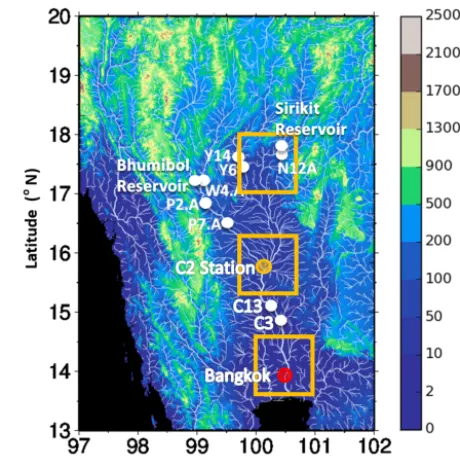
With a catchment area of approximately 158 000 km2, the Chao Phraya River Basin (shown in Fig. 1) is the largest and most important geographical unit in Thailand (Sripong et al., 2000). The northern region of the basin consists of moun-tainous areas; its middle region is a floodplain with a gentle slope of approximately 1/15 000, and its lowermost region is a delta. These geographic features make the region highly prone to flood inundation.

In 2011, enormous economic losses estimated at USD 45 billion (World Bank, 2012) were incurred due to the

Figure 1.The Chao Phraya River Basin. Model domain, elevation map, river network, and validation stations. The orange dot marks the location of the station used for calibration. White dots mark the stations used for validation. The red dot marks the capital of Thai-land, Bangkok. Areas in orange squares are zoomed in for analysis of results.

extensive flooding of Thailand’s industrial zones. The total rainfall during the rainy season was 143 % (∼1439 mm) of that of the average rainy season from 1982 to 2002 (Komori et al., 2012); the flood peaks have exceeded the estimated 100-year return period peak discharges (DHI, 2012). The estimated 16–22 billion m3 of flood volume inundated ap-proximately 14 billion m2of its floodplains (Rakwatin et al., 2013; Mateo et al., 2014). The extent of the damages affected the global supply chain of several industries, particularly the computer and automotive industries (Chongvilaivan, 2012; Swiss Re, 2012). The Thailand flood of 2011 is said to be the most economically damaging flood in recent history (Swiss Re, 2012; EM-DAT, 2015; Munich RE, 2013).

Two huge artificial reservoirs (Bhumibol and Sirikit) and several smaller artificial reservoirs are operational in the Chao Phraya River Basin. In this study, the impacts of reser-voir operation on flood flows are removed by using natural-ized flows (see Appendix for details) and assessing flood ex-tents on dates when both reservoirs are already full and are assumed to have minimal impact on flooding.

3 Methods and data 3.1 CaMa-Flood model

consid-Table 1.CaMa-Flood subgrid parameters in Fig. 1 (based from Ya-mazaki et al., 2011).

Symbol Parameter or variable meaning Unit

Parameters

Ac unit catchment area m2

B bank height m L channel length m W channel width m Z surface altitude m

Variables

Af flooded area m2

Dr river water depth m

Df floodplain water depth m

S total water storage,Sr+Sf m3

Sr river channel water storage m3

Sf floodplain water storage m3

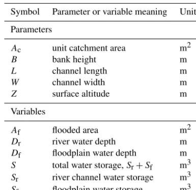
ering floodplain inundation dynamics on the global scale. River basins are discretized and delineated on the desired spatial scale into unit catchments, based on fine-resolution HydroSHEDS flow direction maps (Lehner et al., 2008) and SRTM3 digital elevation models (DEMs; Farr et al., 2007). Each unit catchment is assumed to have a river and flood-plain storage (Fig. 2a, Table 1), the dimensions and charac-teristics of which are calculated using explicit subgrid topog-raphy parameters derived from the fine-resolution flow direc-tion maps and DEM. Gridded runoff from a GCM, GHM, or LSM is used as forcing input to calculate hydrodynamics at each unit catchment within the river basin. River discharge and flow velocity along the river network at each unit catch-ment are calculated using simplified shallow water equations. Water storage (water impounded in river and floodplains) at each unit catchment, the only prognostic variable, is calcu-lated and updated so that water mass is conserved. From the water storage at each time step, other flood inundation char-acteristics such as water level and inundated area are diag-nosed.

The latest and most efficient version of CaMa-Flood (Ya-mazaki et al., 2014b), which uses the “local inertial equa-tion” (Bates et al., 2010) to calculate discharge at each unit catchment, was utilized in this study. By neglecting only the advection term of the 1-D St Venant equation, the lo-cal inertial equation explicitly represents backwater effects and improves the representation of shallow water physics in the model. According to Bates et al. (2010), the local inertial equation can be discretized and modified to Eq. (1),

Qt+1t = Q

t_−1tgAS

1+1tgn2|Qt|

Ah4/3

, (1)

whereQt+1t is the discharge between times t andt+1t, Qt is the discharge at the previous time step,gis the

grav-itational acceleration (m s−2),Ais the flow cross-sectional area (m2),Sis the water surface slope between the upstream and downstream unit catchments,nis the Manning’s friction coefficient (m−1/3s), andhis the flow depth (m).

A new flow scheme, which uses an algorithm to identify and represent diverging channels in a fine-resolution river network map, is incorporated into the latest version of CaMa-Flood (Yamazaki et al., 2014b). By representing the more complex, diverging flows in deltas and floodplains, the new scheme overrules the simplified single downstream connec-tivity (SDC) assumption adopted in most 1-D GRMs. Origi-nally intended to simulate the bifurcation processes in deltas, the new scheme is referred to as the “bifurcation scheme” and the pathways which allow multiple downstream flow as “bi-furcation channels” in the paper by Yamazaki et al. (2014b). Bifurcation channels, defined as channels connecting two unit catchments which do not have upstream–downstream re-lationships in a river network map, are classified as either “overland pathways” (green lines in Fig. 2b) or “river path-ways” (red lines in Fig. 2b).

The algorithm for extracting bifurcation channels is de-scribed in detail in Yamazaki et al. (2014b) and will only be described briefly in this paper. Using data from Hy-droSHEDS and SRTM3, the algorithm searches for possi-ble flow pathways which cross unit-catchment boundaries. A “bifurcation threshold height” above the main channel of each unit catchment is set for computational efficiency. The algorithm searches for pixels (grid cells in the SRTM3 DEM) which are at unit-catchment boundaries and are at an eleva-tion lower than that of the bifurcaeleva-tion threshold. The pixel is identified as a valid bifurcation point if its elevation is higher than that of an adjacent pixel which is located in another unit catchment. Using HydroSHEDS flow directions, a bifurca-tion channel is defined as the pathway from each bifurcabifurca-tion point to the main channel pixels of its upstream and down-stream unit catchments. Bifurcation channels in floodplains are represented by overland pathways, while those with per-sistent bifurcated flow are represented by river pathways. Persistent bifurcated flow is detected using the SRTM wa-ter body data (SWBD) wawa-ter mask (NASA/NGA, 2003). By representing bifurcation channels as described above, flows in braided streams, artificial open canals, diversion channels, and other diverting water pathways can be represented in flood simulations. Hence, the new scheme not only allows the simulation of flows in bifurcating rivers – generally, it enables the simulation of multiple downstream connectivity (MDC) between grid cells. To avoid misconceptions about the function of the new scheme, it will be referred to as “MDC scheme” hereafter. For simplicity, channels or flow pathways which enable MDC are referred to as “MDC chan-nels” or “MDC pathways.”

Figure 2.Schematic diagram of CaMa-Flood.(a)River channel and floodplain subgrid parameters (modified from Yamazaki et al., 2011). Please refer to Table 1 for definition of variables.(b)Subgrid topography and MDC channels. Overland pathways are represented by the green channels while river pathways are represented by the red channels (modified from Yamazaki et al., 2014b).

flows in main channels have been calculated (Yamazaki et al., 2014b).

The development of CaMa-Flood model is well docu-mented and its performance well validated. For more details about the model, please refer to the papers describing its de-velopment (Yamazaki et al., 2011, 2013, 2014b).

3.2 Experiment setup and input data

The FLOW algorithm (Yamazaki et al., 2009) was used to upscale the river network map and calculate the subgrid river channel and floodplain topography in the Chao Phraya River Basin at the following spatial resolutions: 30 arcsec (∼1 km), 1 arcmin (∼2 km), 2 arcmin (∼4 km), 3 arcmin (∼6 km), 4 arcmin (∼8 km), and 5 arcmin (∼10 km). The river and subgrid parameter maps were extracted from the 3 arcsec Hy-droSHEDS flow direction map (Lehner et al., 2008; Lehner and Grill, 2013) and SRTM3 DEM (Farr et al., 2007). Simu-lations were performed at each spatial resolution, switching channel connectivity representation between the SDC and MDC scheme in CaMa-Flood.

To focus on the impacts of spatial resolution and flow processes on the river model, the same daily runoff dataset with a spatial resolution of 5 arcmin square grids was used as forcing input to CaMa-Flood. To conserve the mass of runoff inputs, CaMa-Flood uses area-weighted averaging to distribute the coarse, gridded runoff among the unit catch-ments in CaMa-Flood. The gridded daily runoff dataset was simulated using the land surface processes module of H08 integrated water resources model (Hanasaki et al., 2008a, b; Mateo et al., 2014). The runoff data were simulated using the following meteorological forcing: surface air pressure, wind speed, specific humidity, shortwave radiation, longwave ra-diation, temperature, and surface albedo from a study by Yoshimura et al. (2008), and precipitation data reanalyzed from gauge stations provided by the Royal Irrigation

Depart-ment (RID) and Thai Meteorological DepartDepart-ment (TMD) of Thailand. For further information regarding runoff simula-tion, please refer to Mateo et al. (2014).

The simulation domain was set from 97 to 102◦E lon-gitude and 13 to 20◦N latitude. The calculation time step was automatically adjusted by the Courant–Friedrichs–Lewy condition (see Bates et al., 2010; Yamazaki et al., 2013) in CaMa-Flood. The simulation period was set from 2010 to 2011, with a 1-year spin-up period.

4 Model calibration and validation

The subgrid river cross-section and channel roughness pa-rameters calibrated by Mateo et al. (2014) were used in this study. Parameter tuning and validation were executed by comparing simulation outputs with the surveyed river cross-section and observed river discharge data provided by the RID. Observed satellite images obtained by combining the Moderate Resolution Imaging Spectroradiometer (MODIS) and Advanced Microwave Scanning Radiometer for EOS (AMSR-E) products were used to further tune the subgrid channel parameters and validate the simulated extent of flood inundation (obtained through personal communications from Dr Wataru Takeuchi of the University of Tokyo). These im-ages are available in 10-day intervals at a spatial resolution of 10 arcmin (∼20 km).

The parameterized subgrid river and floodplain topogra-phy as calibrated by Mateo et al. (2014) are shown in Eqs. (2) and (3),

W=max

h

16.6×R0_up.35,3.0

i

, (2)

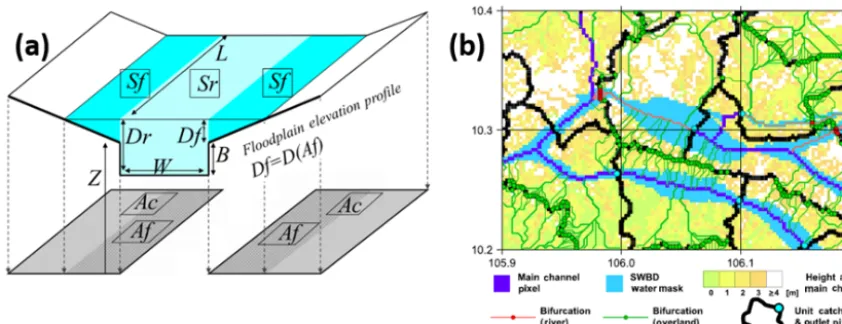
Figure 3.Validation of SDC simulation at 10 km resolution. The simulated(a)daily discharge for the years 2010–2011 and the(b)monthly discharge from 1981–2004 were compared with the naturalized observed discharge. The(c)ratio of inundated area in 25 September 2011 and 25 October 2011 were compared with satellite data. Dam forcing indicates the simulations constrained using actual dam outflows as boundary conditions. All figures were modified from Mateo et al. (2014).

from upstream of the unit catchment (Yamazaki et al., 2011). Based on Mateo et al. (2014), the Manning’s coefficient was fixed at 0.024 in the river channel and 0.10 in the floodplain for the entire basin. These values of Manning’s coefficient are comparable with those used in other studies in the Chao Phraya River Basin (Visutimeteegorn et al., 2007; Keokhum-cheng et al., 2012; Sayama et al., 2015) and those obtained by USGS from lab and field data (Aldridge and Garrett, 1973). By using the calibrated parameters, CaMa-Flood can ade-quately simulate the discharge and flood inundation in the basin (Fig. 3; Mateo et al., 2014).

The model calibrated at 10 km spatial resolution was found to have a good fit with observations. The discharge estimates from the model were in good agreement with the observed river discharge at the station used for calibration (C2 Station in Fig. 1), with the daily Nash–Sutcliffe efficiency (NSE) coefficient in year 2011 with SDC and MDC of 0.73 and 0.80, respectively. The Pearson correlation coefficients be-tween the observed and model-estimated discharge are very high (both above 0.90) and biases are low. There is also a very good agreement between the model-estimated flood

in-undation extents and the satellite-derived water maps for all available satellite images. Validation of the model for differ-ent years and other gauging stations in the Chao Phraya River Basin are also shown to be reasonable by Mateo et al. (2014). The results of the calibration confirm that the parameteriza-tion is reasonably robust and suitable for large-scale applica-tion in the Chao Phraya River Basin. This is to be expected as even without calibration of the parameters, the use of CaMa-Flood with nine GHMs (which include the H08 model) re-sults in better agreement with monthly to daily observations in 1701 globally distributed river discharge stations from the Global Runoff Data Center compared with the native river routing schemes of the GHMs (F. Zhao et al., 2017).

overheads. The stability of the calibration across scales indi-cates that the model is robust.

5 Results

This section starts with a discussion of the impacts of spa-tial scale and representation of MDC on the predictive ca-pability of the model. Subsequently, to explain the causes of the changes in model efficiency, the impacts of scale and representation of MDC on channel topography and flood dy-namics are discussed. For brevity, hereafter, simulations with higher spatial resolution are referred to as “finer resolutions” or “increased resolutions”.

For better visibility when analyzing spatial impacts, we zoomed into the three areas (indicated by the boxes in Fig. 1) located in the upper (up), middle (mid), and lower (low) sec-tions of the catchment. For brevity, only the results in the lower sections of the catchment are shown in this paper.

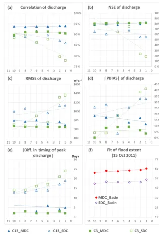
While the results shown in the following subsections are obtained by running the model with calibrated parameters, numerical experiments were also conducted by running the model using alternative parameter values (e.g., parameter values used in global simulations, using the river widths from the global width database for large rivers, GWDLR by Ya-mazaki et al. 2014a). The findings remain the same (and thus are not shown in this paper for brevity), although there are differences in the magnitude of changes in model effi-ciency with changes in spatial resolution. As expected, the use of non-calibrated parameters resulted in larger changes in model efficiency. Hence, the findings of this study are robust and are independent of the parameters used in the model. 5.1 Impacts on predictive capability of the model Six metrics were used to objectively evaluate the predictive capability of the model in each simulation setup: NSE, root mean square error (RMSE), Pearson correlation coefficient (correlation), percent bias (PBIAS), difference in discharge peak timing (in days), and spatial measure of fit of the flood extent (F in Eq. 4, Bates and de Roo, 2000),

F =100×Num(Smod∩Sobs)

Num(Smod∪Sobs)

, (4)

whereSmodandSobsare unit catchments (or pixels) which are

flooded in the model and satellite observation, respectively. The first five metrics evaluate the capability of the model to simulate discharge at the 11 gauge stations (white dots in Fig. 1) while the last evaluates the capability of the model to predict the spatial extent of inundation.

To reduce the impacts of human intervention on the calcu-lated model efficiencies, the observed discharges were nat-uralized as necessary (see Appendix) and flood extent was compared on dates when the dams were filled to their ca-pacity (i.e., minimal effect on downstream flows). Daily dis-charges in the entire year of 2011 were used to calculate the

flow metrics. The flood extent for the month of October 2011 were used to calculate the fit of flood extent,F. To ensure comparability, the simulated flood volumes were projected on the fine-resolution DEM and aggregated to the resolution of the observed satellite images.

It was found that the statistics related to model efficiency do not significantly change in most of the upstream gauging stations. This can be due to at least one of following reasons: (1) the unit catchment is located near or within a mountain-ous area where bank slope is relatively high and where kine-matic wave processes govern more than other flood dynamic processes, and/or (2) MDC pathways are not prevalent and do not significantly affect the simulated flows or inundation. Figure 4 shows that majority of the validation stations are located in regions that have relatively low density of MDC pathways. Hence, the discussions in this section will focus on where the impacts of spatial resolution and complex flows are significant – stations C3 and C13 located in the low-lying floodplain areas.

The changes in model efficiency are more evident in SDC simulations: between simulation at 10 and 1 km resolutions (Fig. 5a–e), NSE and correlation of discharge drastically de-clined by as much as 50 and 10 %, respectively, while RMSE, PBIAS and difference in discharge peak timing drastically increased by as much as 90, 35, and 70 %, respectively. On the other hand, model efficiency incrementally increased and errors marginally decreased with finer resolutions in MDC simulations (below 3 % change between simulations in 10 and 1 km). Although statistically insignificant (less than 5 % between simulations in 10 and 1 km), both MDC and SDC simulations show increasing trends in the fit of flood extent (F shown in Fig. 5f) with finer resolution. In all the six met-rics, MDC simulations consistently outperformed SDC sim-ulations.

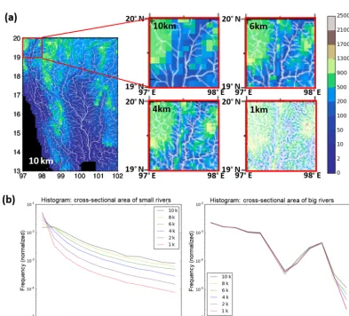
5.2 Impacts on river network and channel topography The river maps (elevation, width, upstream area, and other river channel and floodplain properties) used for simulation are identical between flow connectivity schemes. MDC path-ways were only added to the river maps used for MDC simu-lations. As have been shown in Fig. 4, the number of detected and represented multidirectional pathways increase as reso-lution increases.

Figure 4.Change in the density of MDC pathways with spatial resolution. The density of river network and MDC pathways increase with increasing spatial resolution. Gauge stations upstream of C2 Station (Y14, Y6, N12A, W4A, P2A, and P7A) are located in zones with low density of MDC pathways. Gauge stations C2, C13, and C3 are located in low-lying and floodplain areas which have a high density of MDC pathways.

The equations used to parameterize the subgrid river widths and bank heights (see Eqs. 2 and 3 in the previous section) are dependent on a fixed minimum width and bank heights and the annual maximum runoff in the subcatchment area upstream of the unit catchment (Yamazaki et al., 2011). Because the same runoff data (GRDC-based for the param-eterization) was used to generate the river maps, the sub-grid topography of river channels which have been identi-fied in coarser resolution maps did not significantly change in finer resolution maps. These river channels typically have large cross-sectional areas (river width≥100.0 m, river bank height ≥2.0 m; called main channels hereafter). However, the discretization process resulted in an increase in the pro-portion of small river channels (river width<100.0 m, river

bank height <2.0 m; called main small streams hereafter) represented in finer resolution maps.

5.3 Impacts on flood inundation and flow characteristics

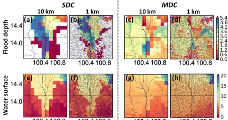
Generally, the increasing discretization of the river basin in finer resolution maps led to increasingly defined flood depths and flood extents (see Fig. 7) and hence the increasing fit of flood extent,F, in both SDC and MDC simulations. This can be mainly attributed to the more defined representation of topographical details in finer spatial resolutions.

as-Figure 5.Model efficiency at varying spatial resolution and varying flow connectivity schemes. The statistics for discharge (correlation, RMSE, percent bias, NSE coefficient, and difference in peak timing) were calculated and compared with the naturalized discharge at corre-sponding gauge stations. The fit of flood extent was calculated for the entire basin.

sumption used in SDC simulations constrained the flow of water within subcatchments that have upstream–downstream relationships. This resulted in unrealistic flood inundation patterns and water surface elevation in SDC simulations: wa-ter surface elevation in a very flat portion of the river basin shown in Fig. 7e, f reveals unlikely flood boundaries and abrupt drops of more than 5 m in elevation.

These effects are avoided by allowing water flows between adjacent floodplains that do not have explicit upstream– downstream channel relationships through MDC pathways.

As a result, more widespread flood extent with more realis-tic, gradually decreasing water surface elevation is obtained in MDC simulations (Fig. 7g, h). Flood inundation in unit catchments with main channels became less severe in MDC simulations than those in SDC simulations (last two columns and first two columns in Fig. 7, respectively).

Table 2.Statistical information on the subgrid characteristics of river channels.

River characteristic Map resolution Trend∗ 10 km 8 km 6 km 4 km 2 km 1 km

Number of land unit catchments 4534 7068 12 541 28 178 112 447 449 285 ↑

Ratio (wide river) 0.15 0.12 0.09 0.07 0.03 0.02 ↓

Ratio (narrow river) 0.85 0.88 0.91 0.93 0.97 0.98 ↑

Ratio (deep river) 0.19 0.15 0.12 0.08 0.04 0.02 ↓

Ratio (shallow river) 0.81 0.85 0.88 0.92 0.96 0.98 ↑

Max. width (m) 326.62 326.62 326.62 326.62 326.62 326.62 — Mean width (wide river) 167.33 166.77 167.22 166.94 167.31 167.32 — Mean width (narrow river) 36.52 32.93 28.62 23.47 16.44 11.26 ↓

Max. height (m) 4.96 4.96 4.96 4.96 4.96 4.96 — Mean height (deep river) 2.96 2.95 2.95 2.96 2.95 2.95 — Mean height (shallow river) 1.09 1.01 0.92 0.81 0.63 0.49 ↓

∗_{↑: increasing;↓: decreasing; —: no significant change.}

Figure 7.Impacts of spatial resolution and representation ofMDCon simulated flood depth and water surface.(a–d)Flood depth and(e– h)water surface at the lower part of the basin. The first two columns show the results for SDC simulations at 10 and 1 km resolutions while the last two columns show the results for MDC simulations.

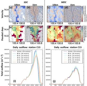
intermittent compared with those in SDC simulations. In ef-fect, flood duration became longer at finer resolutions in SDC simulations, as shown in Fig. 8e, f. The simulated hydrograph at C13 station shown in Fig. 8i reveals decreasing outflows with increasing resolution in the rising limb and a reversal of this trend in the recession limb. The difference in time to peak with increasing resolution is also evident in the SDC-simulated hydrographs. Such patterns are subdued or not ev-ident in MDC simulations (Fig. 8j).

6 Discussion

6.1 Importance of representing multiple downstream connectivity

Most global flood models use discharge outputs from a cou-pling of GHMs or GCMs and 1-D GRMs in their cascade of models (e.g., ECMWF by Pappenberger et al., 2012, GloFRIS by Ward et al., 2013 and Winsemius et al., 2013, JRC by Dottori et al., 2016). Before the development of CaMa-Flood with the MDC scheme, runoff in most GRMs is routed throughout the land mass by discretizing the river basin into grids or smaller subcatchments, where each grid or subcatchment is assumed to have one river channel that flows to one downstream channel (SDC assumption). This means that an upstream–downstream relationship between two grids is necessary for water to flow between them. By using this simplified approach, runoff generated by GHMs or GCMs can be routed throughout the basin and can be calculated in large domains.

The older generation of GRMs which use the SDC as-sumption were designed to simplify the representation of network and flows in continental rivers and to run at rela-tively coarse spatial resolutions (coarser than 10 km grid res-olution). At coarse spatial resolutions, one grid cell may be large enough to cover an area with a river delta (its main channel and braided streams or tributaries). In such cases, the grid cell may be assumed to flow towards one direction, most likely towards the direction of the next main channel; hence, the SDC flow scheme may be sufficient to represent the river network and flows realistically. However, this as-sumption may be too simplified or inappropriate for repre-senting the flow network in deltas and braided streams when we move to finer spatial resolution simulations.

Figure 8.Impacts of spatial resolution and representation of MDC to(a–d)flow velocity,(e–h)number of days of flooding in a year, and (i–j)2011 daily outflows (river+floodplain flows) at C13 Station. Panels(a–h)show simulation results at the lower part of the basin.

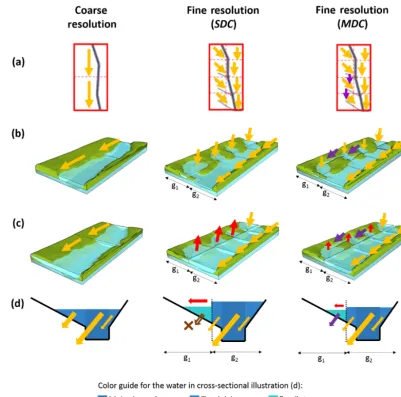
In the event of flooding, floodplains in coarse-resolution simulations (left-most column, Fig. 9a–c) will be filled with water that is at the same level as that of in main chan-nels. Water in floodplains flow in the same direction as the main channel (yellow orange arrows in Fig. 9). On the other hand, in finer resolution SDC simulations, the floodplains are discretized into unit catchments with “small streams” (teal cross-section of the middle figure in Fig. 9d). These small streams will be filled with water which can only flow through its small channel towards (or away from) the main channel; water cannot flow in the same direction as the main channel (brown arrows in Fig. 9d). In effect, the capacity of flood-plains to allow water to flow through (hereby referred to as flow capacity) to the downstream channel is significantly re-duced in finer resolution SDC simulations. Multidirectional flow connectivity reduces the effect of this phenomenon. With the presence of MDC pathways, water in small streams can flow both towards the main channel and the direction of the MDC pathway (purple arrows in Fig. 9); hence, similar

flow capacity to in coarser simulations can be maintained in finer MDC simulations.

In the occurrence of a flood wave, water level in the main channels at finer resolutions will become higher than the up-stream “small rivers.” When this occurs in SDC simulations, water can only flow backwards in the small rivers. This ex-plains the severe and widespread “build up” of backflows in SDC simulations in Fig. 8b, and the “trapping” of water which leads to longer simulated flood days in Fig. 8f. The massive backflows are avoided in MDC simulations (evident in Fig. 8c, d, g, and h) because MDC pathways allow wa-ter to flow to surrounding grids other than the main channel (purple arrows in Fig. 9).

Figure 9.Schematic diagram of the initial distribution of water in coarse and fine resolution simulations.(a)Top view of the river flow network.(b)Isometric 3-D representation of the section of the river. Here, to visualize the small rivers and main channels, vertical features of the floodplain are illustrated with exaggeration. Arrows depict flow direction during non-flood conditions.(c)Isometric and(d) cross-sectional illustration of the flow direction in the river network during flooding. Yellow orange arrows indicate the flow of water to the downstream, purple arrows indicate flow in MDC pathways, red arrows indicate backflows, and brown arrows succeeded by “×” marks indicate no flow connectivity in that direction.

slopes, single-downstream-grid river channel and floodplain flows will not be able to realistically simulate the spreading of water in very flat floodplains and deltas. MDC pathways are not only useful for representing braided or bifurcating streams in coarser resolution simulations – they are neces-sary for representing and maintaining flow connectivity and flow capacity in very flat floodplains in finer resolution sim-ulations.

6.2 On improved simulation of large-scale floods at finer resolutions

Small catchment-scale topographic controls and flow pro-cesses are critical in regulating the storage and movement

of surface waters (Yamazaki et al., 2011; Neal et al., 2012b). While finer resolution modeling leads to improved represen-tation of topography, simulation of large-scale floods using GRMs will not necessarily improve through hyper-resolution modeling alone – GRMs will have to be improved by suffi-cient representation of flow physics (both subgrid and be-tween grids) which are appropriate for the scale of imple-mentation.

was found to be sufficient in simulating extensive flooding in the test basin. CaMa-Flood sufficiently represents both to-pographic controls and flow processes in large-scale simula-tions through (1) subgrid parameterization of river and flood-plain topography, (2) use of local inertial equation in calcu-lating 1-D channel and floodplain flows, and (3) representa-tion of multiple downstream connectivity of flows.

While the application of GRMs in a cascade of large-to global-scale models large-to finer spatial resolution is ideal, it is important to note that they are not meant to replace catchment-scale flood models. Where more detailed local data are available, catchment-scale hydrodynamic models are more suitable for thorough planning and exploration of management and mitigation options on local scales (Ward et al., 2015; Teng et al., 2017). Catchment-scale hydrody-namic models usually have a more complete representation of surface water flow physics compared to global models. Although more detailed hydrodynamic models can simulate flood processes more accurately, their implementation in re-gional to global domains entails high computational costs; the models either have to be implemented at coarser reso-lutions or re-configured to simplify their representation of flow processes (Horritt and Bates, 2001; Hunter et al., 2007). The predictive capability of hydrodynamic models deteri-orates when implemented at coarser resolutions (Kirchner, 2006; Neal et al., 2012a, b). The governing physical equa-tions in these models are not applicable to more complex, heterogenous systems in larger domains (Kirchner, 2006), and most of the key topographic controls within the flood-plain are smeared when aggregated to coarser scales. While several catchment-scale hydrodynamic models have already been applied to large river basins by representing subgrid to-pographical controls at coarser resolutions (e.g., Wilson et al., 2007; Neal et al., 2012b), such application still requires a significant amount of boundary data processing and compu-tational resources when coupled with GCMs and GHMs (Ya-mazaki et al., 2014b). Such applications of catchment-scale hydrodynamic models to coarse spatial resolution simulation of large-scale floods are not shown to be superior to those from advanced GRMs. To harness the benefits from using GRMs and catchment-scale hydrodynamic models, the de-velopment of hybrid approaches, where outputs from CaMa-Flood with the MDC scheme are used as initial or boundary conditions of catchment-scale hydrodynamic models, may be developed and assessed in the future. Hybrid approaches us-ing relatively simpler GRMs have been shown to be feasible in the continental- to global-scale mapping of flood hazards and risks at fine spatial resolution (e.g., Ward et al., 2013; Winsemius et al., 2013; Dottori et al., 2016).

6.3 Caveats and future works

One of the caveats of this study is the tedious calibra-tion of the subgrid channel parameters when applied to re-gional basins. On the global scale, this can potentially be

ad-dressed by the global width database available for large rivers (GWDLR, developed by Yamazaki et al., 2014a). A database of channel depths of large rivers, however, does not exist; hence, the parameters characterizing the channel depths in the model may still have to be calibrated. To ease the dif-ficulty of calibration, the development of an automatic cali-bration tool or a simpler or more efficient parameterization of subgrid channels (e.g., Neal et al., 2015) may be helpful.

In the test basin used in this study, it was found that the parameters calibrated at a coarse spatial resolution are trans-ferable across finer spatial resolutions. This significantly re-duces the time required to re-calibrate the model at finer spa-tial resolutions. Once the inispa-tial difficulty of calibrating the necessary parameters at a coarse spatial resolution is hurdled, CaMa-Flood with MDC scheme can be used for more real-istic, consistent, and robust simulation of large-scale floods across varying spatial resolutions. It should be noted, how-ever, that the MDC scheme of CaMa-Flood had only been validated in three test basins – Mekong delta (Yamazaki et al., 2014b), Ganges–Brahmaputra–Meghna delta (Ikeuchi et al., 2015) and Chao Phraya River Basin in Thailand (this study). It should also be noted that the transferability of cal-ibrated parameters from a coarse spatial resolution to finer spatial resolutions have to be validated in other river basins. More extensive tests in large river basins and on global scales have to be conducted to further validate the model.

and other geological processes, or by levee breaks, water diversion, and other anthropogenic impacts) and operation of artificial canals are not represented in the current model. Such natural or anthropogenic influences which add to the complexities in real flow pathways have significant impacts on the connectivity and flood dynamics in floodplains (Syvit-ski et al., 2005; Alsdorf et al., 2007; Schumann et al., 2011; Trigg et al., 2013). However, even catchment-scale hydro-dynamic models implemented at fine spatial resolution have difficulties in representing such complex processes. The rep-resentation of such complexities will require the integration of more detailed models and data (e.g., landscape, sedimen-tation, anthropogenic) with flood models.

Other than representing MDC in a 1-D model, there are other model structures which can realistically simulate flood dynamics in large floodplains, such as those that implement full St Venant momentum equations (e.g., Paiva et al., 2011, 2013). For the benefit of developing reduced-complexity models which can adequately simulate large-scale floods in finer resolution, more model structures should also be as-sessed in the future.

The limited availability of inundation data for validation of flood extent on large scales, especially in data-poor regions, is another caveat of this study. The satellite-derived inunda-tion product used in this study is too coarse to comprehen-sively assess the capability of the model to simulate flood inundation parameters at varying spatial resolutions. Better flood satellite images available on large scales and at finer spatial and temporal resolutions will certainly be beneficial for such analyses.

The relatively coarse runoff forcing data are also another issue that needs to be addressed. Similar to most studies done in the past (e.g., Kumar et al., 2006; Famiglietti et al., 2009), this study is largely constrained by the lack of mete-orological forcing datasets at finer resolutions. The authors tested the use of finer resolution runoff data generated from simple spatial interpolations with topographical correction in the meteorological data, but no significant results have been found (and hence, were not shown in this study for the sake of brevity). However, finer resolution runoff data generated from better and finer inputs can potentially improve results in other river basins. Previous studies have already shown that using finer spatial resolution inputs could result in improve-ments in runoff and water balance calculations (Kumar et al., 2006; Singh et al., 2015). In this regard, a study which in-volves varying resolution of runoff inputs, subgrid river and floodplain topographical maps, and model implementation may be conducted in the future.

7 Conclusion

In this study, we have assessed the suitability and demon-strated the capability of an advanced GRM for simulating flood discharge and inundation at finer spatial resolutions. Both the impacts of more realistic representation of down-stream flow connectivity and finer spatial resolution have been assessed. While the predictive capability of the model improved slightly with finer spatial resolution when multi-ple downstream flow is considered, it declined significantly when single downstream flow, the flow connectivity scheme used in most GRMs, is used. To keep the level of simulation skill of a GRM at finer spatial resolutions, an appropriate set of physical representations should be included in the model. In this study, it was found that representing multiple down-stream flow connectivity is important in the realistic simu-lation of inundation in floodplains, especially at finer spa-tial resolutions. MDC pathways provide two essenspa-tial func-tions in simulation of large-scale flood inundation: (1) rep-resentation of flow connectivity between floodplains which allow more realistic flood routing in deltas and low-lying flat lands and (2) maintenance of the flow capacity in floodplains and river channels across varying spatial scales. These re-sults clearly show that with regards to large-scale modeling of flood inundation in very flat floodplains and deltas, (1) finer resolution modeling will not always result in better pre-dictions and (2) multidirectional flow connectivity is one of the important flow processes that have to be represented in the model structure.

Appendix A: Methodology for and stability of calibration

There are several long-standing issues regarding parameter calibration in flood inundation models. Parameters that give a high efficiency (e.g., NSE, correlation coefficient) do not necessarily result in low errors (e.g., RMSE, PBIAS) nor high predictive capability of simulating flood extent; mul-tiple good parameter sets may also exist (equifinality prob-lem; Beven, 2002; Pappenberger et al., 2005; Yamazaki et al., 2011). Hence, the calibrated parameter set may give good overall results but may not always perform best in all mea-sures of efficiency. Therefore, the focus of this section is not to test whether the calibrated coefficients will result in opti-mal performance in all metrics; rather, it examines whether the optimal coefficients in one spatial scale remain to be so in the other spatial scale.

CaMa-Flood and H08 models were calibrated by increas-ing the NSE-coefficient in monthly and daily discharges, re-ducing the errors in the timing and magnitude of peak dis-charge during the worst drought and worst flood year in the dataset, and comparing the spatiotemporal characteristics of flood extent. The calibration of parameters using discharge was carried out at Nakhon Sawan Station, also known as C2 Station (marked by an orange dot in Fig. 1), a gauging station critically located just after the confluence of the four main tributaries of the Chao Phraya River Basin. The simulated daily and monthly discharge hydrographs are compared with that of the naturalized observed to remove the effects of the operation of Bhumibol and Sirikit reservoirs. The naturalized observed discharge was computed by deducting the effects of reservoir operation upstream of the station using Eq. (A1), NDC2=ODC2+ [I+P−R−S]Bhumibol

+ [I+P−R−S]_Sirikit, (A1)

where ND is naturalized discharge, OD is observed dis-charge, I is reservoir inflow, P is water pumped into the reservoir, R is reservoir release, and S is water released through the spillway. Gauging stations within the basin with observation years greater than 10 and catchment area greater than 10 000 km2have been chosen for the validation (marked by white dots in Fig. 1). Similarly, the observed discharge in validation stations downstream of either Bhumibol or Sirikit Reservoirs were naturalized using Eq. (A1), modified ac-cordingly, before comparison with the simulated discharge. For further details on calibration and validation, please refer to Mateo et al. (2014).

The CaMa-Flood model can be calibrated and tuned by changing coefficientsxw,yw,zw,xb,yb, andzbin Eqs. (A2)

and (A3): W =max

xw×Rupyw, zw, (A2)

B=maxxb×Rupyb, zb. (A3)

As previously mentioned,W is the river width,B is the river bank height, andRup is the annual maximum 30-day

moving average runoff from upstream of the unit catchment (Yamazaki et al., 2011). The model is quite sensitive to the subgrid channel parameters. A sensitivity analysis done by Yamazaki et al. (2011) showed that a deeper bank height, wider channel width, or smaller Manning’s coefficient re-sult in less flooded area and larger fluctuations and advanced peaks in simulated discharge.

To reduce the complexity of calibrating multiple parameter coefficients, the parameters were calibrated by keeping four of the six coefficients constant while varying the two remain-ing coefficients: (1) coefficients of the river width,xwandyw;

(2) coefficients of the river bank height,xb andyb; and (3)

coefficients of minimum river width and bank height,zwand

zb. To test the robustness of the calibrated parameters, the

parameters were perturbed by varying two coefficients ac-cording to Fig. A1 while keeping the other four coefficients equal to the previously calibrated coefficients by Mateo et al. (2013, 2014). In total, 24 parameter sets are tested (pa-rameter sets W5, B5, and WB5 are similar to the calibrated parameters). To verify the stability of the calibration with varying spatial scales, the numerical experiment was carried out at two resolutions: (1) 10 km (base simulation) and (2) 4 km.

The parameter sets were evaluated based on the following metrics: Pearson correlation coefficient, NSE, PBIAS, dif-ference in the magnitude of peak discharge, difdif-ference in the timing of the peak discharge, and fit of flood extent (for the entire basin compared with satellite images on 25 October 2011). Thresholds (values in parentheses) were set to deter-mine the acceptable parameter sets: high correlation coeffi-cient (above 60 %), high NSE (above 60 %), low PBIAS (ab-solute value below 10 %), low error in peak magnitude (less than 10 %), low error in date to peaking (less than 10 days), and high flood extent statistics. The ‘optimum’ parameter set was determined by (1) calculating the performance of each parameter set in each metric, (2) screening out parameter sets that do not satisfy all of the thresholds used for evaluation, (3) ranking the remaining parameter sets in each metric, (4) giving equal weight to each metric to obtain the simple av-erage rank of the parameter sets, and (5) getting the highest ranking (low rank value) parameter set.

Table A1 summarizes the results of the ranking for param-eter sets W1 to W9 and B1 to B9 for the two spatial resolu-tions. It was found that the model is not sensitive to changes in coefficientszwandzb(similar to the results of sensitivity

Figure A1.Parameter sets used in checking the transferability of calibration at 10 and 4 km spatial resolutions.

Table A1.Summary of mean ranks for each parameter set at 10 and 4 km spatial resolution. Abbreviated codes indicate that the parameter set had been screened out in at least one of the criteria used for evaluation.

Parameter set Mean rank

B(10 km) W(10 km) B(4 km) W(4 km)

1 Pt Pm, Pt B, Pm, Pt Pm, Pt

2 Pt Pt Pm, Pt Pm, Pt

3 Pt 2 Pt 1

4 Pt Pt Pt Pm, Pt

5 2 1 1 2

6 4 Pm 4 Pm

7 1 Pt 2 Pm, Pt

8 3 3 3 3

9 N, Pm, Pt N, Pm, Pt N, Pm, Pt N, Pm, Pt

Reasons for screening out the parameter set from the ranking: N – low NSE, B – high bias, Pm– high difference in the magnitude of peak discharge, and Pt– high difference in the

timing of peak discharge

within 10 % difference in size compared with those produced using the calibrated parameter set. Hence, the results confirm that the “optimum” parameter set do not significantly change with spatial scale. This is most likely due to the use of the same runoff data, Rup, to calculate the subgrid

Code and data availability. The CaMa-Flood model is available upon request. Terms and conditions for use and download are available at the following website: http://hydro.iis.u-tokyo.ac.jp/ ~yamadai/cama-flood/index.html (Yamazaki, 2014, Yamazaki et al., 2014b). The DEM and hydrographic data used in this study can be downloaded from https://dds.cr.usgs.gov/srtm/version2_1/ (SRTM, USGS, 2013a; Farr et al., 2007) and https://hydrosheds. cr.usgs.gov/dataavail.php (HydroSHEDS, USGS, 2013b; Lehner et al., 2008). The discharge data used for validation were ob-tained from the Royal Irrigation Department of Thailand (http:// hydrologydb.rid.go.th/water/discharge/index.htm; RID, 2011). The runoff data used as input to the model are outputs from the H08 model (outputs from 1981–2004 are available here: http://impact-di. eng.ku.ac.th/products/public/H08/; IMPAC-T, 2013). The discharge and runoff data were obtained through the Integrated study on Hydro-Meteorological Prediction and Adaptation to Climate Change in Thailand (IMPAC-T) project.

Competing interests. The authors declare that they have no conflict of interest.

Acknowledgements. This study was supported by the Japan Society for the Promotion of Science KAKENHI (16H06291) and the Integrated study on hydroMeteorological Prediction and Adaptation to Climate change in Thailand (IMPAC-T) Project through the Science and Technology Research Partnership for Sustainable Development (SATREPS). We are thankful to all the people, especially the Thai government officials, who have provided the hydrologic data which were used to calibrate and validate the models in this study. We are also grateful to the two anonymous referees who have provided constructive comments which led to improvements in the paper. The main author is also grateful to her thesis panelists, Toshio Koike, Hiroaki Furumai, Yukiko Hirabayashi, and Naota Hanasaki, who have critically examined and thereby significantly contributed to the scientific merit of this study, as well as the Commonwealth Scientific and Industrial Research Organisation (CSIRO) for providing support.

Edited by: Alberto Guadagnini Reviewed by: two anonymous referees

References

Adhikari, P., Hong, Y., Douglas, K. R., Kirschbaum, D. B., Gourley, J., Adler, R., and Brakenridge, G. R.: A digitized global flood inventory (1998–2008): compilation and preliminary results. Nat. Hazards, 55, 405–422, https://doi.org/10.1007/s11069-010-9537-2, 2010.

Aldridge, B. N. and Garrett, J. M.: Roughness coefficients for stream channels in Arizona (No. 73-3), US Geological Survey, United States Department of the Interior Geological Survey, Tuc-son, Arizona, 1973.

Alfieri, L., Burek, P., Dutra, E., Krzeminski, B., Muraro, D., Thie-len, J., and Pappenberger, F.: GloFAS – global ensemble stream-flow forecasting and flood early warning, Hydrol. Earth Syst.

Sci., 17, 1161–1175, https://doi.org/10.5194/hess-17-1161-2013, 2013.

Alsdorf, D., Bates, P., Melack, J., Wilson, M., and Dunne, T.: Spatial and temporal complexity of the Amazon flood measured from space. Geophys. Res. Lett., 34, L08402, https://doi.org/10.1029/2007GL029447, 2007.

Balsamo, G., Pappenberger, F., Dutra, E., Viterbo, P., and van den Hurk, B.: A revised land hydrology in the ECMWF model: a step towards daily water flux prediction in a fully-closed water cycle, Hydrol. Process., 25, 1046–1054, https://doi.org/10.1002/hyp.7808, 2011.

Bates, P. D. and De Roo, A. P. J.: A simple raster based model for flood inundation simulation, J. Hydrol., 236, 54–77, https://doi.org/10.1016/S0022-1694(00)00278-X, 2000. Bates, P. D., Horritt, M. S., and Fewtrell, T. J.: A simple inertial

formulation of the shallow water equations for efficient two-dimensional flood inundation modelling, J. Hydrol., 387, 33–45, https://doi.org/10.1016/j.jhydrol.2010.03.027, 2010.

Beven, K.: Towards a coherent philosophy for modelling the environment, P. Roy. Soc. Lond. A Mat., 458, 2465–2484, https://doi.org/10.1098/rspa.2002.0986, 2002.

Beven, K. J. and Cloke, H. L.: Comment on “Hyper-resolution global land surface modeling: Meeting a grand challenge for monitoring Earth’s terrestrial water” by Eric F. Wood et al., Water Resour. Res., 48, W01801, https://doi.org/10.1029/2011WR010982, 2012.

Bierkens, M. F.: Global hydrology 2015: State, trends, and directions, Water Resour. Res., 51, 4923–4947, https://doi.org/10.1002/2015wr017173, 2015.

Brakenridge, G. R.: “Global Active Archive of Large Flood Events”, Dartmouth Flood Observatory, University of Colorado, http://floodobservatory.colorado.edu/Archives/index.html, last access: March 2015.

Chongvilaivan, A.: Thailand’s 2011 flooding: Its impact on di-rect exports, and disruption of global supply chains, in: ART-NET Policy Brief No. 34, UN Economic and Social Commis-sion for Asia and the Pacific, Bangkok, available at: http:www. artnetontrade.org (last access: March 2015), 2012.

DHI: MIKE FLOOD User Manual, DHI Software 2005, DHI Water & Environment, Denmark, 2005.

DHI: Thailand Floods 2011 – The Need for Holistic Flood Risk Management, DHI-NTU Res. Cent., Singapore, 2012.

Di Baldassarre, G. and Uhlenbrook, S.: Is the current flood of data enough? A treatise on research needs for the im-provement of flood modelling, Hydrol. Process., 26, 153–158, https://doi.org/10.1002/hyp.8226, 2011.

Döll, P., Kaspar, F., and Lehner, B.: A global hydrological model for deriving water availability indicators: model tuning and vali-dation, J. Hydrol., 270, 105–134, https://doi.org/10.1016/S0022-1694(02)00283-4, 2003.

Dottori, F. and Todini, E.: Developments of a flood inun-dation model based on the cellular automata approach: testing different methods to improve model perfor-mance, Phys. Chem. Earth, Parts A/B/C, 36, 266–280, https://doi.org/10.1016/j.pce.2011.02.004, 2011.

EM-DAT: EM-DAT: International Disaster Database by Guha-Sapir, D., Below, R., and Hoyois, Ph., Université Catholique de Louvain, Brussels, Belgium, available at: http:www.emdat.be, last access: March 2015.

Falter, D., Dung, N. V., Vorogushyn, S., Schröter, K., Hundecha, Y., Kreibich, H., Apel, H., Theisselmann, F., and Merz, B.: Continuous, large-scale simulation model for flood risk as-sessments: proof-of-concept, J. Flood Risk Manage., 9, 3–12, https://doi.org/10.1111/jfr3.12105, 2016.

Famiglietti, J. S., Murdoch, L., Lakshmi, V., and Hooper, R. P.: Towards a framework for community modeling in hydrologic science: Blueprint for a community hydrologic modeling plat-form, paper presented at 2nd Workshop on a Community Hydro-logic Modeling Platform, Univ. of Memphis, Memphis, Tenn., 31 March to 1 April, 2009.

Farr, T. G., Rosen, P. A., Caro, E., Crippen, R., Duren, R., Scott, H., Kobrick, M., Paller, M., Rodriguez, E., Roth, L., Seal, D., Shaf-fer, S., Shimada, J., Umland, J., Werner, M., Oskin, M., Burbank, D., and Alsdorf, D.: The Shuttle Radar Topography Mission, Rev. Geophys., 45, RG2004, https://doi.org/10.1029/2005RG000183, 2007.

Hanasaki, N., Kanae, S., Oki, T., Masuda, K., Motoya, K., Shi-rakawa, N., Shen, Y., and Tanaka, K.: An integrated model for the assessment of global water resources – Part 1: Model description and input meteorological forcing, Hydrol. Earth Syst. Sci., 12, 1007–1025, https://doi.org/10.5194/hess-12-1007-2008, 2008a. Hanasaki, N., Kanae, S., Oki, T., Masuda, K., Motoya, K.,

Shi-rakawa, N., Shen, Y., and Tanaka, K.: An integrated model for the assessment of global water resources – Part 2: Applica-tions and assessments, Hydrol. Earth Syst. Sci., 12, 1027–1037, https://doi.org/10.5194/hess-12-1027-2008, 2008b.

Hirabayashi, Y., Kanae, S., Emori, S., Oki, T., and Kimoto, M.: Global projections of changing risks of floods and droughts in a changing climate, Hydrol. Sci. J., 53, 754–772, https://doi.org/10.1623/hysj.53.4.754, 2008.

Hirabayashi, Y., Mahendran, R., Koirala, S., Konoshima, L., Ya-mazaki, D., Watanabe, S., Kim, H., and Kanae, S.: Global flood risk under climate change, Nat. Clim. Chang., 3, 816–821, https://doi.org/10.1038/nclimate1911, 2013.

Horritt, M. S. and Bates, P. D.: Effects of spatial resolution on a raster based model of flood flow. J. Hydrol., 253, 239–249, https://doi.org/10.1016/S0022-1694(01)00490-5, 2001. Hunter, N. M., Bates, P. D., Horritt, M. S., and Wilson,

M. D.: Simple spatially-distributed models for predicting flood inundation: A review, Geomorphology, 90, 208–225, https://doi.org/10.1016/j.geomorph.2006.10.021, 2007. Ikeuchi, H., Hirabayashi, Y., Yamazaki, D., Kiguchi, M., Koirala,

S., Nagano, T., Kotera, A., and Kanae, S.: Modeling com-plex flow dynamics of fluvial floods exacerbated by sea level rise in the Ganges–Brahmaputra–Meghna Delta, En-viron. Res. Lett., 10, 124011, https://doi.org/10.1088/1748-9326/10/12/124011, 2015.

IMPAC-T: H08 Dataset, Integrated study on Hydro-Meteorological Prediction and Adaptation to Climate Change in Thailand (IMPAC-T), Oki-Lab, IIS, The University of Tokyo, Japan and IMPAC-T Project Office, Kasetsart University, Thailand, avail-able at: http://impact-di.eng.ku.ac.th/products/public/H08/, last access: September 2013.

Keokhumcheng, Y., Tingsanchali, T., and Clemente, R. S.: Flood risk assessment in the region surrounding the Bangkok Suvarnabhumi Airport, Water Int., 37, 201–217, https://doi.org/10.1080/02508060.2012.687868, 2012.

Kirchner, J. W.: Getting the right answers for the right rea-sons: Linking measurements, analyses, and models to advance the science of hydrology, Water Resour. Res., 42, W03S04, https://doi.org/10.1029/2005WR004362, 2006.

Komori, D., Nakamura, S., Kiguchi, M. Nishijima, A., Yamazaki, D., Suzuki, S., Kawasaki, A., Oki, K., and Oki, T.: Character-istics of the 2011 Chao Phraya River flood in Central Thailand, Hydrol. Res. Lett., 6, 41–46, https://doi.org/10.3178/HRL.6.41, 2012.

Kumar, S. V., Peters-Lidard, C. D., Tian, Y., Houser, P. R., Geiger, J. Olden, S., Lighty, L., Eastman, J. L., Doty, B., Dirmeyer, P., Adams, J., Mitchell, K., Wood, E. F., and Sheffield, J.: Land in-formation system: An interoperable framework for high resolu-tion land surface modelling, Environ. Modell. Softw., 21, 1402– 1415, https://doi.org/10.1016/j.envsoft.2005.07.004, 2006. Lehner, B. and Grill, G.: Global river hydrography and

net-work routing: baseline data and new approaches to study the world’s large river systems, Hydrol. Process., 27, 2171–2186, https://doi.org/10.1002/hyp.9740, 2013.

Lehner, B., Verdin, K., and Jarvis, A.: New Global Hydrography Derived From Spaceborne Elevation Data, Eos Trans. AGU, 89, 93–94, https://doi.org/10.1029/2008EO100001, 2008.

Mateo, C., Hanasaki, N., Komori, D., Yoshimura, K., Kiguchi, M., Champathong, A., Sukhapunnaphan, T., Yamazaki, D., and Oki, T.: A simulation study on modifying reservoir operation rules: Tradeoffs between flood mitigation and water supply, in: Consid-ering Hydrological Change in Reservoir Planning and Manage-ment (IAHS Publ. 362), edited by: Schumann, A., 33–40, IAHS Press, Wallingford, UK, 2013.

Mateo, C. M., Hanasaki, N., Komori, D., Tanaka, K., Kiguchi, M., Champathong, A., Sukhapunnaphan, T., Yamazaki, D., and Oki, T.: Assessing the impacts of reservoir operation to floodplain inundation by combining hydrological, reservoir management, and hydrodynamic models, Water Resour. Res., 50, 7245–7266, https://doi.org/10.1002/2013WR014845, 2014.

Munich RE: Significant natural catastrophes 1980–2012: 10 costliest floods worldwide ordered by overall losses, Münch-ener Rückversicherungs-Gesellschaft, Geo Risks Res., Nat-CatSERVICE, Munich, Germany, available at: https://www. munichre.com/touch/touchnaturalhazards/ (last access: March 2015), 2013.

NASA/NGA: SRTM Water Body Data Product Specific Guidance, Version 2.0, available at: http://dds.cr.usgs.gov/srtm/version2_ 1/SWBD/SWBD_Documentation/ (last access: February 2014), 2003.

Neal, J., Villanueva, I., Wright, N., Willis, T., Fewtrell, T., and Bates, P.: How much physical complexity is needed to model flood inundation? Hydrol. Process., 26, 2264–2282, https://doi.org/10.1002/hyp.8339, 2012a.

Neal, J., Schumann, G., and Bates, P.: A sub-grid channel model for simulating river hydraulics and floodplain inundation over large and data sparse areas, Water Resour. Res., 48, W11506, https://doi.org/10.1029/2012WR012514, 2012b.

incorpora-tion of channel cross-secincorpora-tion geometry uncertainty into regional and global scale flood inundation models, J. Hydrol., 529, 169– 183, https://doi.org/10.1016/j.jhydrol.2015.07.026, 2015. Oki, T. and Sud, Y. C.: Design of Total Runoff

Integrat-ing Pathways (TRIP)–A global river channel network, Earth Interactions, 2, 1–37, https://doi.org/10.1175/1087-3562(1998)002<0001:DOTRIP>2.3.CO;2, 1998.

Paiva, R. C. D., Collischonn, W., and Tucci, C. E. M.: Large scale hydrologic and hydrodynamic modeling using limited data and a GIS based approach, J. Hydrol., 406, 170–181, https://doi.org/10.1016/j.jhydrol.2011.06.007, 2011.

Paiva, R. C. D., Collischonn, W., and Buarque, D. C.: Vali-dation of a full hydrodynamic model for large-scale hydro-logic modelling in the Amazon, Hydrol. Process., 27, 333–346, https://doi.org/10.1002/hyp.8425, 2013.

Pappenberger, F., Beven, K., Horritt, M., and Blazkova, S.: Uncertainty in the calibration of effective rough-ness parameters in HEC-RAS using inundation and downstream level observations, J. Hydrol., 302, 46–69, https://doi.org/10.1016/j.jhydrol.2004.06.036, 2005.

Pappenberger, F., Dutra, E., Wetterhall, F., and Cloke, H. L.: Deriv-ing global flood hazard maps of fluvial floods through a phys-ical model cascade, Hydrol. Earth Syst. Sci., 16, 4143–4156, https://doi.org/10.5194/hess-16-4143-2012, 2012.

Petrescu, A. M. R., van Beek, L. P. H., van Huissteden, J., Prigent, C., Sachs, T., Corradi, C. A. R., Parmentier, F. J. W., and Dol-man, A. J.: Modeling regional to global CH4emissions of

bo-real and arctic wetlands, Glob. Biogeochem. Cy., 24, GB4009, https://doi.org/10.1029/2009gb003610, 2010.

Rakwatin, P., Sansena, T., Marjang, N., and Rungsipanich, A.: Using multi-temporal remote-sensing data to esti-mate 2011 flood area and volume over Chao Phraya River basin, Thailand, Remote Sens. Lett., 4, 243–250, https://doi.org/10.1080/2150704X.2012.723833, 2013.

RID: RID-Hydrology System (Discharge), Royal Irrigation Depart-ment, Bangkok, Thailand, available at: http://hydrologydb.rid. go.th/water/discharge/index.htm (last access: September 2013), 2011.

Sampson, C. C., Bates, P. D., Neal, J. C., and Horritt, M. S.: An automated routing methodology to enable direct rainfall in high resolution shallow water models, Hydrol. Process., 27, 467–476, https://doi.org/10.1002/hyp.9515, 2013.

Sampson, C. C., Smith, A. M., Bates, P. D., Neal, J. C., Alfieri, L., and Freer, J. E.: A high-resolution global flood hazard model, Water Resour. Res., 51, 7358–7381, https://doi.org/10.1002/2015wr016954, 2015.

Sampson, C. C., Smith, A. M., Bates, P. D., Neal, J. C., and Trigg, M. A.: Perspectives on Open Access High Resolution Digital El-evation Models to Produce Global Flood Hazard Layers, Front. Earth Sci., 3, 85, https://doi.org/10.3389/feart.2015.00085, 2016. Sayama, T., Tatebe, Y., Iwami, Y., and Tanaka, S.: Hydrologic sen-sitivity of flood runoff and inundation: 2011 Thailand floods in the Chao Phraya River basin, Nat. Hazards Earth Syst. Sci., 15, 1617–1630, https://doi.org/10.5194/nhess-15-1617-2015, 2015. Schumann, G. J. P., Neal, J. C., Mason, D. C., and Bates, P. D.:

The accuracy of sequential aerial photography and SAR data for observing urban flood dynamics, a case study of the UK summer 2007 floods, Remote Sens. Environ., 115, 2536–2546, 2011.

Schumann, G. J. P., Bates, P. D., Neal, J. C., and Andreadis, K. M.: Technology: Fight floods on a global scale, Nature, 507, 169– 169, https://doi.org/10.1038/507169e, 2014.

Singh, R. S., Reager, J. T., Miller, N. L., and Famiglietti, J. S.: Toward hyper-resolution land surface modeling: The effects of fine-scale topography and soil texture on CLM4.0 simulations over the southwestern U.S., Water Resour. Res., 51, 2648–2667, https://doi.org/10.1002/2014WR015686, 2015.

Sood, A. and Smakhtin, V.: Global hydrological mod-els: a review, Hydrol. Sci. Journ., 60, 549–565, https://doi.org/10.1080/02626667.2014.950580, 2015.

Sripong, H., Khao-uppatum, W., and Thanopanuwat, S.: Flood man-agement in Chao Phraya River Basin, in: Proceedings of the In-ternational Conference on The Chao Phraya Delta: Historical De-velopment, Dynamics and Challenges of Thailand’s Rice Bowl, Kasetsart Univ., Bangkok, available at: http://www.std.cpc.ku.ac. th/delta/deltacp/home.htm (last access: August 2012), 2000. Swiss Re: Natural catastrophes and man-made disasters in 2011:

Historic losses surface from record earthquakes and floods, Sigma, 2, Swiss Reinsurance Co. Ltd., Econ. Res. and Con-sult., Zurich, Switzerland, available at: http://media.swissre. com/documents/sigma2_2012_en.pdf (last access: March 2014), 2012.

Syvitski, J. P., Kettner, A. J., Correggiari, A., and Nelson, B. W.: Distributary channels and their im-pact on sediment dispersal, Mar. Geol., 222, 75–94, https://doi.org/10.1016/j.margeo.2005.06.030, 2005.

Teng, J., Vaze, J., Dutta, D., and Markanek, S.: Rapid inundation modelling in large floodplains using LiDAR DEM, Water Re-sour. Manage., 29, 2619–2636, https://doi.org/10.1007/s11269-015-0960-8, 2015.

Teng, J., Jakeman, A. J., Vaze, J., Croke, B. F. W., Dutta, D., and Kim, S.: Flood inundation modelling: A review of methods, re-cent advances and uncertainty analysis, Environ. Modell. Softw., 90, 201–216, https://doi.org/10.1016/j.envsoft.2017.01.006, 2017.

Trigg, M. A., Michaelides, K., Neal, J. C., and Bates, P. D.: Surface water connectivity dynamics of a large scale extreme flood, J. Hydrol., 505, 138–149, https://doi.org/10.1016/j.jhydrol.2013.09.035, 2013.

Trigg, M. A., Birch, C. E., Neal, J. C., Bates, P. D., Smith, A., Sampson, C. C., Yamazaki, D., Hirabayashi, Y., Pappenberger, F., Dutra, E., and Ward, P. J.: The credibility challenge for global fluvial flood risk analysis, Environ. Res. Lett., 11, 094014, https://doi.org/10.1088/1748-9326/11/9/094014, 2016.

USGS (U.S. Geological Survey): Shuttle Radar Topography Mis-sion (SRTM), U.S. Department of the Interior, USA, avail-able at: https://hydrosheds.cr.usgs.gov/dataavail.php, last access: September 2013a.

USGS (U.S. Geological Survey): HydroSHEDS, U.S. Department of the Interior, USA, available at: https://hydrosheds.cr.usgs.gov/ dataavail.php, last access: September 2013b.

van Beek, L. P. H., Wada, Y., and Bierkens, M. F.: Global monthly water stress: 1. Water balance and water availability, Water Resour. Res., 47, W07517, https://doi.org/10.1029/2010WR009791, 2011.